Towards Whole Body Fatigue Assessment of Human Movement: A Fatigue-Tracking System Based on Combined sEMG and Accelerometer Signals


Abstract
: This paper proposes a method to assess the overall fatigue of human body movement. First of all, according to previous research regarding localized muscular fatigue, a linear relation is assumed between the mean frequency and the muscular working time when the muscle is experiencing fatigue. This assumption is verified with a rigorous statistical analysis. Based on this proven linearity, localized muscular fatigue is simplified as a linear model. Furthermore, localized muscular fatigue is considered a dynamic process and, hence, the localized fatigue levels are tracked by updating the parameters with the most current surface electromyogram (sEMG) measurements. Finally, an overall fatigue level is computed by fusing localized muscular fatigue levels. The developed fatigue-tracking system is evaluated with two fatigue experiments (in which 10 male subjects and seven female subjects participated), including holding self-weight (dip start position training) and lifting weight with one arm (arm curl training).
1. Introduction
In the field of biomechanics, fatigue is defined as a decrease in physical movement performance due to internal and external forces [1]. Cumulative physical fatigue can lead to musculoskeletal disorders (MSD) [2]. Thus, monitoring and tracking fatigue is of great importance in order to prevent the development of such disorders. Many applications benefit from fatigue monitoring, such as promoting muscle performance and growth in sports training [3]; preventing intolerant exercise in rehabilitation [4,5], etc. In this paper, we propose a method to assess the overall fatigue status of human movement and verify the proposed method by a prototype. An extensive body of literature exists on the subject of monitoring localized muscular fatigue, thus our proposed method is based on this research. Our final objective is to provide a solution to the assessment of human fatigue statuses in whole body movements. In this paper, we focus on developing a prototype of a wearable fatigue-tracking system to quantify overall fatigue in a specific human movement.
Existing approaches to the monitoring of muscular fatigue can be categorized into two types: simulation-based and experiment-based. Regarding the simulation-based methods, numerous muscular fatigue models have been built according to the Ca2+ cross-bridge mechanism [6,7], force-PH relation [8,9], elastic element modeling (e.g., Hill's model) [10], etc. However, for experiment-based methods, the use of surface electromyogram (sEMG), a non-invasive technique, has become popular in clinical fatigue measurement, as the subject experiences minimal discomfort while measuring fatigue levels (no needle punctures are required) [11,12]. Studies from the field of kinesiology have shown that the power spectrum variables (including mean frequency, median frequency, and mode frequency) [13] of the sEMG signal decrease during sustained contraction. In practice, the mean frequency of the sEMG signal has been widely used for detecting muscular fatigue due to its low sensitivity to noise [14,15]. Several computational methods for calculating the mean frequency from the power spectrum have been introduced in literature, including classical methods (e.g., the periodogram, and the Blackman-Tukey estimator) and modern parametric model methods (such as autoregressive, moving average, autoregressive moving average, etc.) [16].
Since our method and prototype must be functional in practical applications, we adopt the experiment-based methods. Specifically, we use the mean frequency to indicate localized muscular fatigue due to its low sensitivity to noise [6]. This paper targets at the quantification and monitoring of the overall fatigue status of human body movement based on localized muscular fatigues. Furthermore, we treat “overall fatigue” as a dynamic process and, thus, it is updated by the most current sEMG measurements. The following issues are addressed in detail in this paper:
Quantifying an overall fatigue assessment corresponding with a human movement: The current literature regarding fatigue addresses the problem either at the muscle level [17] or at the joint level [18]. Fatigue assessment at the muscle level is commonly considered fatigue classification. Different classifiers can be applied, such as the neural network (NN) classifier, the Bayesian classifier, the fuzzy logic (FL) classifier, the support vector machine (SVM) classifier, and the hidden Markov model (HMM) classifier [19]. On the other hand, the fatigue assessment at the joint level is usually simplified to a first-order differential process of the current joint load torque divided by the maximum joint load [18,20]. In this paper, we address on assessing “overall fatigue level” corresponding to a specific human movement. More specifically, we fuse the muscle fatigue levels by weighted average, where the weight defined here is customized case by case due to different applications. As an example in our research, the weight is set as a normalized gradient of the muscular fatigue level.
Tracking fatigue status: In previous research, muscular fatigue is essentially considered a static process, as it is assessed only by the current measurements [3,12]. However, fatigue is naturally a dynamic process, meaning that a previous fatigue status also influences a current fatigue status. Thus, we introduce a “forgetting factor”, whose physical meaning is the amount of previous fatigue status information that should be considered [21]. In this paper, we propose a tracking method of muscular fatigue based on the concept of dynamically “forgetting previous fatigue information”. In computation, as the current muscular fatigue status is iteratively updated by the fatigue information at the previous time step and most current measurement, it has low sensitivity to disturbances.
This paper is organized as follows: in Section 2, we describe the system architecture, basic scheme, experimental setting and signal pre-possessing; in Section 3, we illustrate segmentation and connection of the sEMG signals by detecting periodic movements; in Section 4, we describe the statistical analysis and simplification of the localized muscular fatigue level; in Section 5, we present the tracking scheme of the localized muscular fatigue levels and their fusion to generate an overall fatigue level; in Section 6, the verification of our proposed method is illustrated by the fatigue tracking performance in two fatigue experiments; and in Section 7, we conclude the paper and provide plans for our future work.
2. System Architecture and Experiment Setting
2.1. Hardware
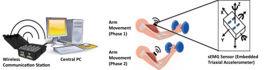
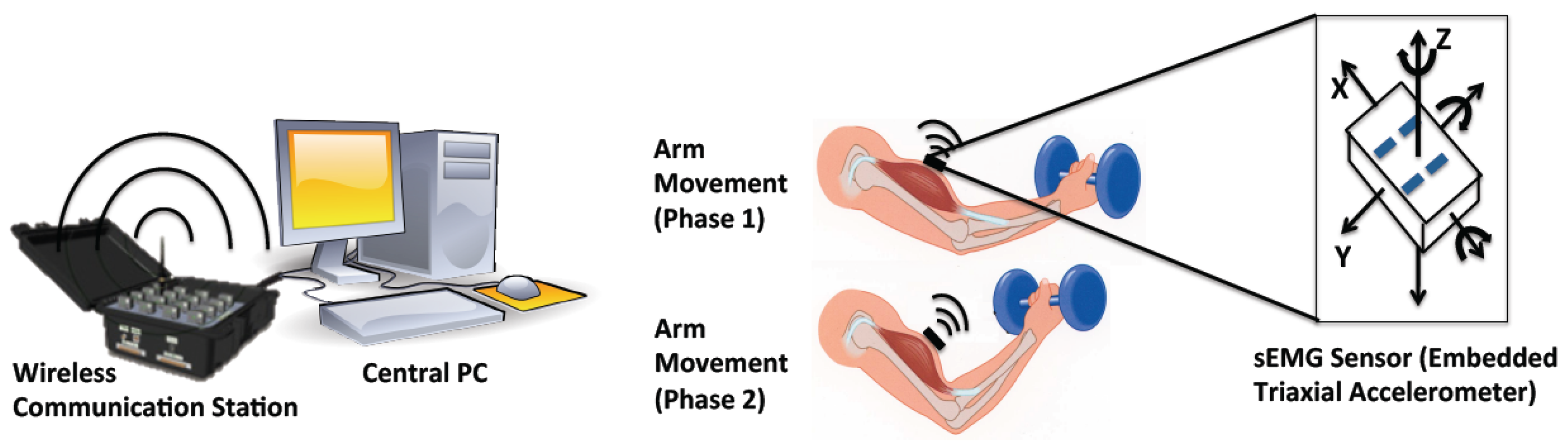
The fatigue-tracking system includes a central processing PC, a wireless communication center and a couple of sEMG sensors (Figure 1). The sEMG sensor used is a Delsys Trigno wireless sensor (37 mm × 26 mm × 15 mm, 16-bit resolution, 2,000 Hz sampling rate), which consists of a parallel-bar-based EMG measurement device and a triaxial accelerometer. The triaxial accelerometer is used to capture dynamic movements and impact simultaneously with the sEMG data measurements.
As the sEMG sensor is required to be placed at the center of the muscle during the muscle's contraction, the body movement can be monitored by an accelerometer. The wireless communication center (maximum communication distance is 40 m) is used to receive the online data from the sEMG sensors and send it to the central processing PC. It can simultaneously communicate with 16 sEMG sensors (i.e., having 16 EMG channels, 48 accelerometer channels). The central PC computes and displays the tracked fatigue level by human interactive interface.
2.2. Basic Scheme
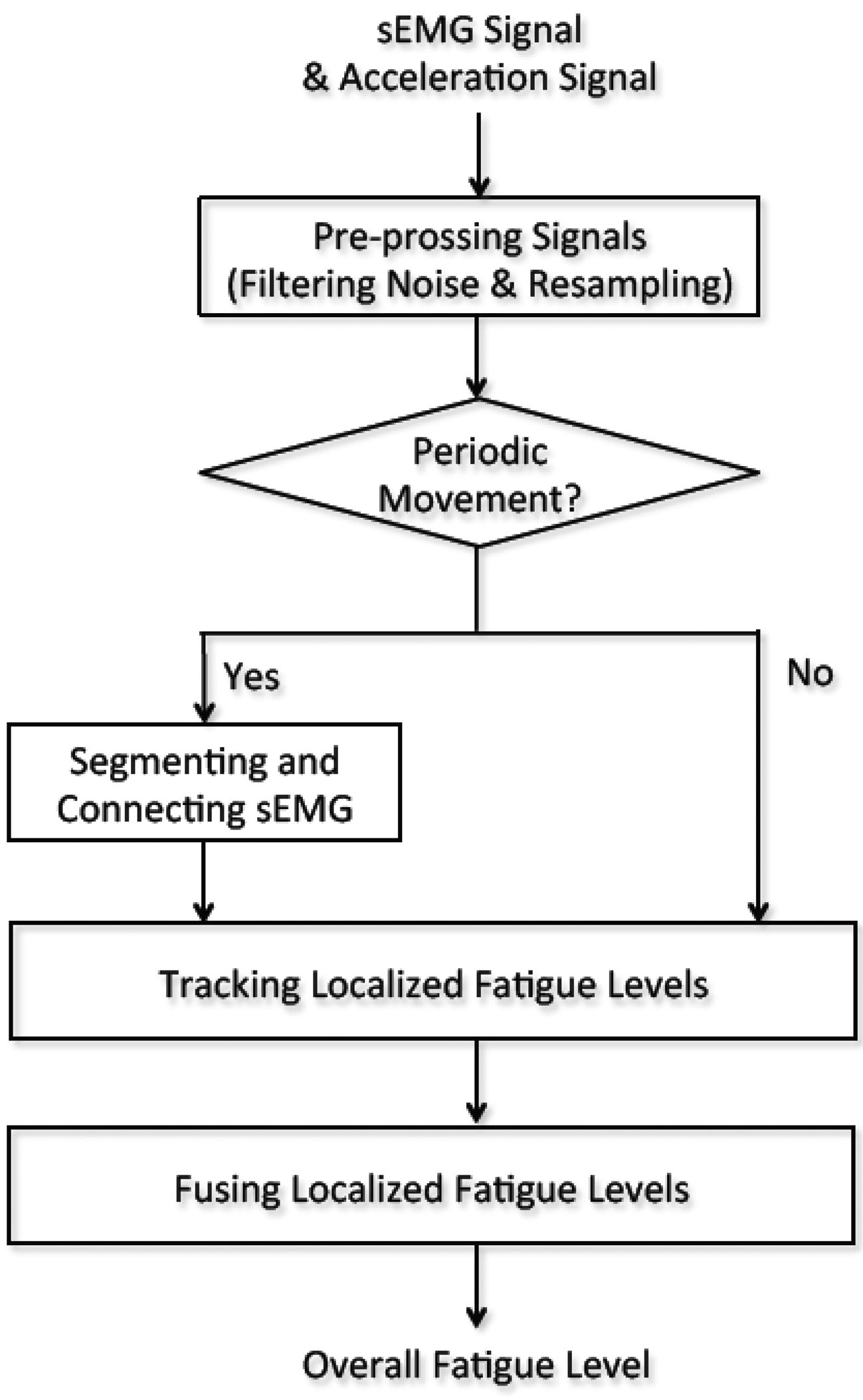
The sEMG signal processing is performed in a central PC and illustrated in Figure 2. Initially, the sEMG signal and corresponding acceleration signal are filtered to remove high frequency noise. Next, the two signals are re-sampled so that both signals have the same sampling rates. The filtered acceleration signal is then used to recognize periodic movements. If periodic movements are detected, the filtered sEMG signal is segmented and connected to form a new sEMG signal for mean frequency calculation. The localized fatigue levels are then tracked by updating the parameters with the most current sEMG measurement. If there is no periodic movement recognized, the sEMG segmentation and connection procedure is skipped. Finally, the overall fatigue level is computed by fusing the localized fatigue levels. The details of this method are outlined in Sections 3–5.
2.3. Experimental Procedures
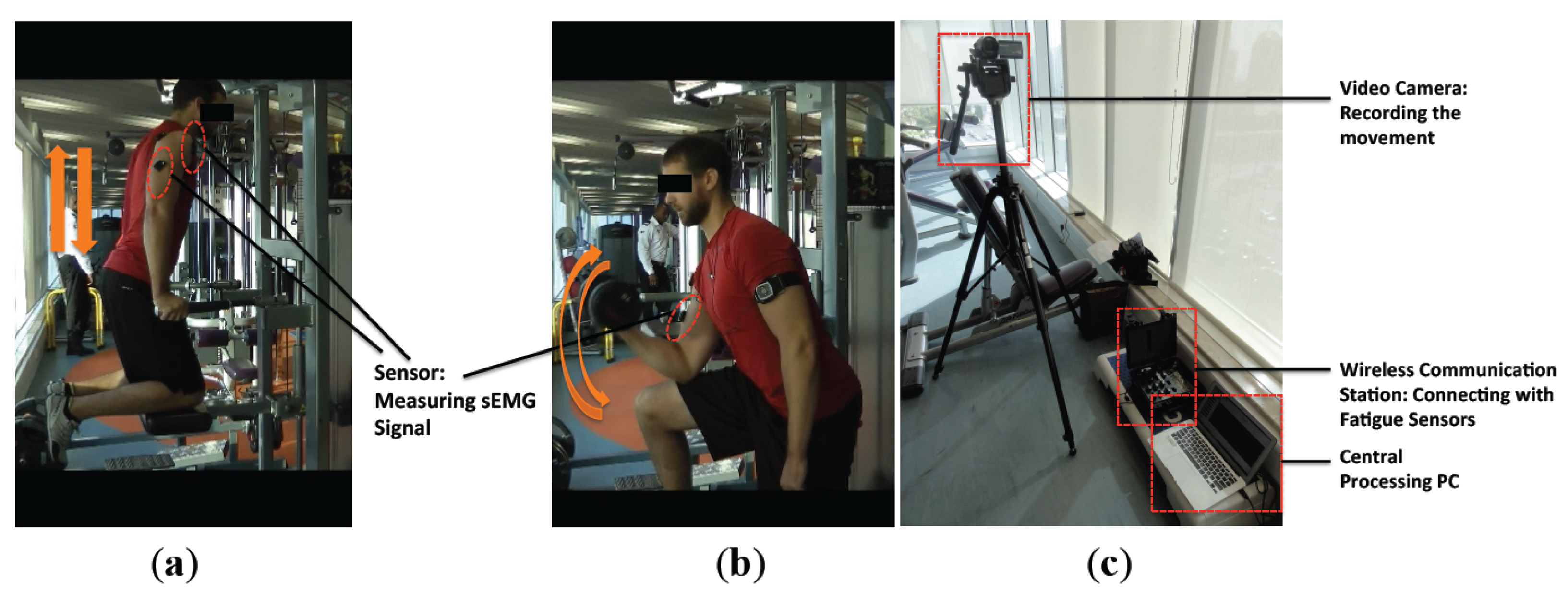
We conducted two experiments for the verification of our method (Figure 3). The experiment procedures have been approved by the university's committee. In Experiment 1, the subjects are asked to hold their self-body weight with both arms for a period of time (dip start position training); in Experiment 2, the subjects were asked to periodically lift a weight (10 kg for males, and 6 kg for females) with their right arm (arm curl training). In total, 17 subjects, including 10 males and 7 females, were studied (mean ± SD): age 30.47 ± 6 years; body mass 71.71 ± 16.81 kg; body height 172.82 ± 11.25 cm; and body mass index (BMI) 23.86 ± 4.03 kg/m2. Before initiating the experiment, the subjects were briefed with the experiment's purpose and procedures. The subjects were asked to attach the sEMG sensors on the following muscle groups: biceps brachii, anterior deltoids, and triceps brachii. Taking into account the muscles measured in the experiments, shaving body hair were not necessary. The skin of each subject was cleaned with 90% alcohol and then the sensors were attached using double faced adhesive tape (based on the instructions of the Delsys sensors).
After warming up, each subject was required to hold their self-body weight for 1 min in Experiment 1 (Figure 3a) where the angle between lower arm and upper arm is approximately 120°, rest for 5–10 min, and then periodically lift a weight (complete bending-stretching movement) with the right arm approximately every 2.5 s during a 1 min time span in Experiment 2 (Figure 3b). Lifting pace was roughly informed by rhythmic sound. Here, the maximum duration of 1 min was determined due to the arm-shaking phenomenon that appeared for all the subjects before 1 min, which clearly indicated the subjects' high fatigue status.
During the experiments, the sEMG signals were measured and further transferred to the central processing PC via a wireless communication station where the signal processing was executed in Matlab. The whole experiment process was recorded by a video camera (Figure 3c).
2.4. Pre-Processing Signals
The sEMG signal and the acceleration signal are filtered using the Butterworth filter. Specifically, in designing the Butterworth filter, the lowest order of the filter n and normalized cutoff frequency Wn are firstly computed by the designed filter parameters, including passband corner frequency Wp, stopband corner frequency Ws, passband ripple Rp, and stopband attenuation Rs. After that, the Butterworth filter is determined by n and Wn. According to the feature of sEMG and acceleration signals in our designed fatigue experiments, the filter specifications of the two signals are set as follows: for sEMG signal, Wp = 0.1 Hz, Ws = 0.4 Hz, Rp = 3 dB, Rs = 40 dB; for acceleration signal, Wp = 0.003 Hz, Ws = 0.006 Hz, Rp = 3 dB, Rs = 40 dB. The settings of the moving window are as follows: the window length is 0.125s and the window overlap is 0.063 s. In our system, the sampling rate of the sEMG signal and the acceleration signal is 4,000 Hz and 296 Hz, respectively. To ensure the two signals have the same data length in analysis, the measured sEMG signal is resampled in the rate of 4,000/296.
3. Automatic Periodic Movement Detection
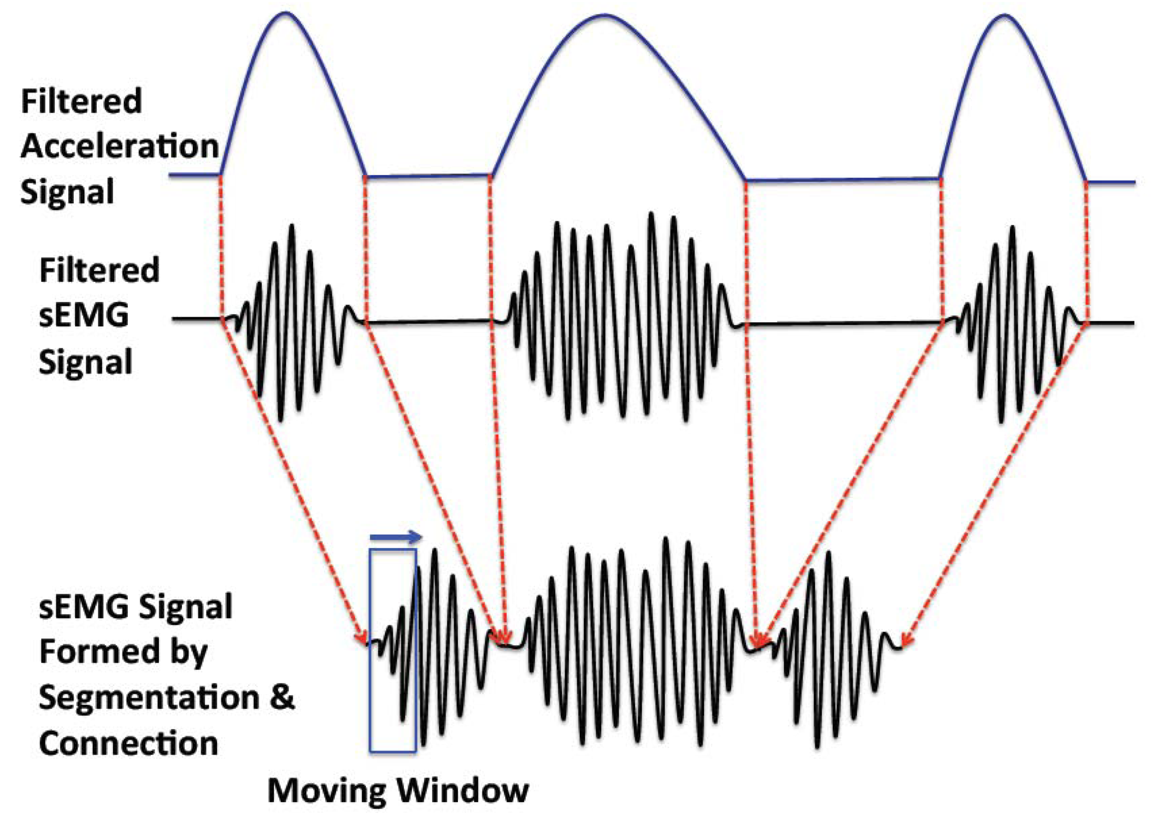
There are two working patterns in muscle movement: sustained contraction (considered as non-periodic movement) and alternate contraction-recovery (considered as periodic movement) [12]. The former is simpler to analyze, as it is a continuous and consistent movement pattern; the latter is more complex, as it consists of a contraction and a recovery phase, corresponding with active sEMG and inactive sEMG signals, respectively. To assess the muscular fatigue of the alternate contraction-recovery muscle movement, we segment the contraction movement and connect the corresponding active sEMG signals (Figure 4).
Although the periodic movement pattern can possibly be detected by the sEMG signal, this pattern is much clearer when the acceleration signal is used. In the following part, we apply correlation analysis on the acceleration signal in order to detect the periodic movement. In detail, we use the cross-covariance to analyze the acceleration signal to detect if the recorded movement is a periodic movement and, if so, to find out the breaking points for segmentation.
In detail, for the acceleration signal ACC with N samples, we compute the cross-covariance ϕACC by [16]:
Otherwise, a non-periodic movement is confirmed. Here, Max(i,j) returns the j-th largest value in the vector i. ε is a threshold determining the periodic movement judge.
4. Modeling Localized Fatigue Level
First of all, we define the localized fatigue level as:
According to previous literature on mean frequency for time-series analysis [19], we assume that the mean frequency decreases linearly with working time as the fatigue gradually increases [14,15], i.e.:
Hφ0: φt = 0 (meaning that working time is not a useful predictor of mean frequency change)
Hφ1: φt ≠ 0 (meaning that working time is a useful predictor of mean frequency change)
We apply analysis of variance (ANOVA) on the measurement data of Experiment 1 to prove the above hypotheses in Table 1 where m1 to m10 and f1 to f7 are the subject number in male and female group respectively. p is the significance number.
It is shown that all the p values in Table 1 are less than 0.05 and, thus, we reject the null hypothesis Hφ0. This means that the variation explained by the linear model is not due to random chance. Meaning that we have evidence to conclude that the slope parameter φt is not 0, and hence it can be a predictor of fmean,i. In other words, considering the individual differences and the above verification, the linear model (Equation (6)) is suitable for describing mean frequency of different individuals. Based on the linear model of the mean frequency in Equation (6), we can simplify the localized fatigue level as:
5. Tracking and Fusing Localized Muscular Fatigue Levels
According to the statistical analysis outlined in the previous section, φt is an adequate predictor of fmean,i. Thus, we can track the muscular fatigue level lfatigue by identifying the slope φt. As φt is a time-varying coefficient, we estimate its value at each moment. Here, the estimation model of the mean frequency can be formed as:
Here, φ̂t can be obtained by minimizing the total error between the real and estimated model in the sense of least-squares, i.e.:
In detail, by defining pt = t−2, we can rewrite Equation (10) as:
With Equations (11) and (12), we can update φ̂t by using φ̂t−1 and the most current measurement fmean,i. From the work done by Branch and Evan [23], the least squares with forgetting is a restricted form of the Kalman filter with constant gain equaling to 1− λ.
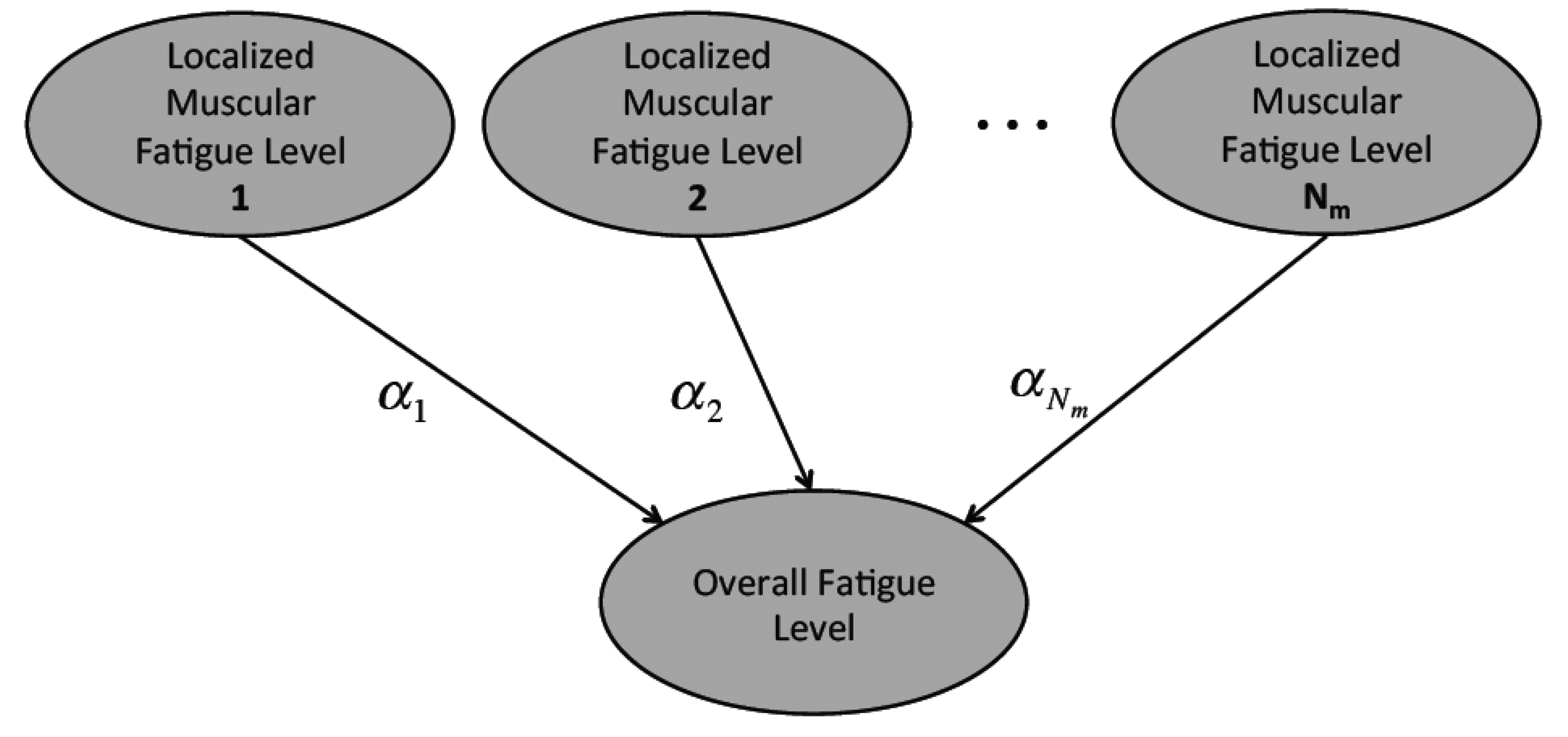
The tracked localized muscular fatigue levels are further fused to define the overall fatigue level of a human body movement (Figure 5) where Nm is the total muscle number and αi (i = 1, 2,…, Nm) is the weight coefficient. In detail, the localized muscular fatigue level fusion can be calculated by:
The procedures of overall fatigue level computation are summarized in Algorithm 1 as follows:
| Algorithm 1: Overall fatigue level computation | |
| Input: Raw sEMG and corresponding acceleration signals | |
| Output: Overall fatigue level | |
| 1: | Filter and resample the input signals; |
| 2: | For i from 1 to Nm |
| 3: | Calculate the self-covariance of the filtered acceleration signal ϕACC; |
| 4: | If ϕACC < ε, the movement is recognized as a periodic movement. Then, the corresponding sEMG signal is segmented and connected to form a new sEMG signal, otherwise, do nothing; |
| 5: | Compute the initial mean frequency of the sEMG signal fmean,0; |
| 6: | Initialize λ, φ̂t and pt. φ̂t(0) can be 0 or an initial guess of the slope parameter, as pt is defined as t−2, pt(0) has to be set as a relatively large number; |
| 7: | Compute fmean,i and update φ̂t and pt by Equations (11) and (12); |
| 8: | Calculate the localized fatigue level lfatigue,i by Equation (9); |
| 9: | End For |
| 10: | Compute the overall fatigue level lfatigue by lfatigue,i (Equation (13)). |
6. Results and Discussion
In the following Sections from 6.1 to 6.4, we take one subject's case to discuss the fatigue-tracking results. In Section 6.5, we summarize the outcomes from all the participants and evaluate the developed system.
6.1. Measurement
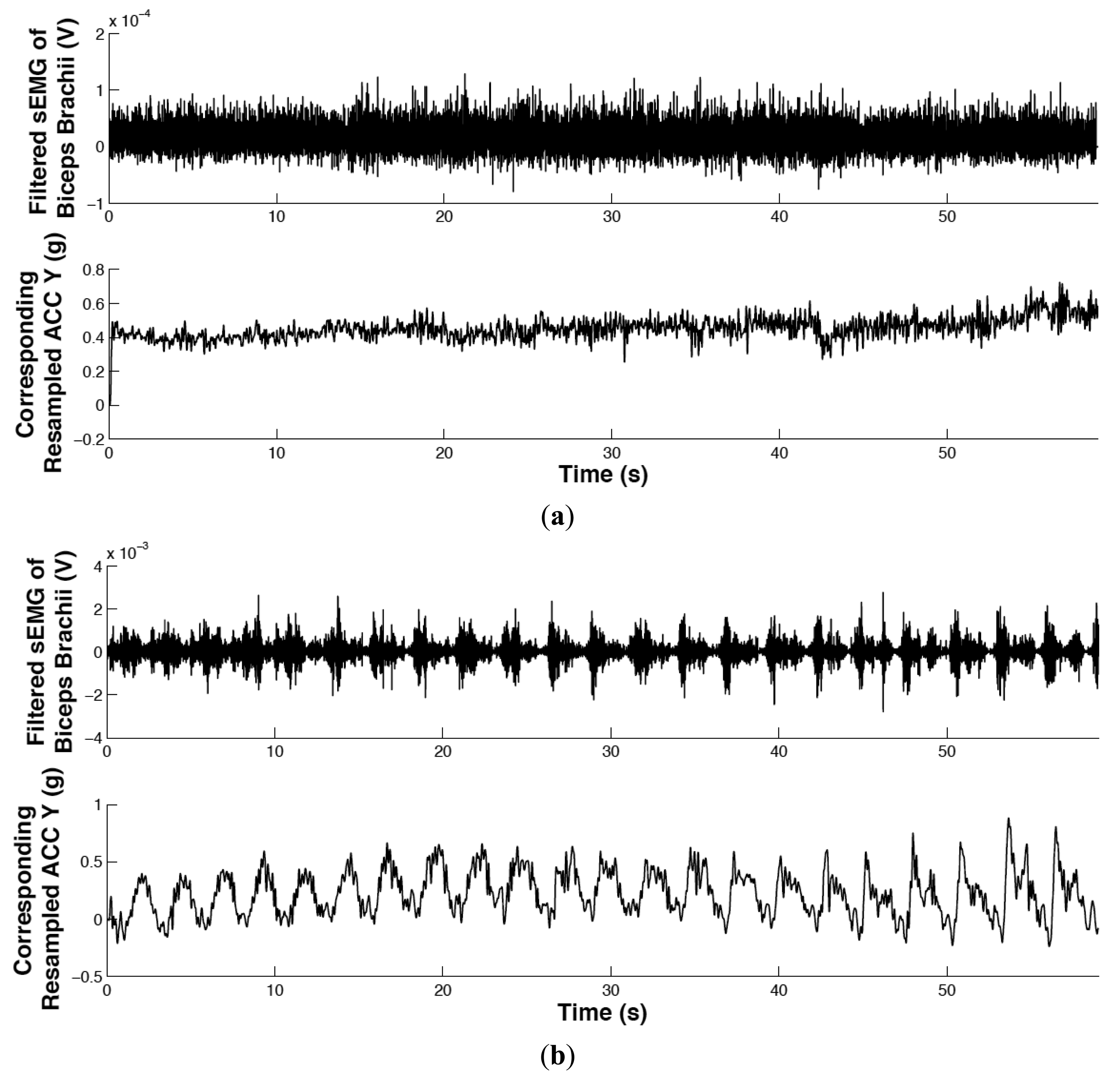
The filtered sEMG signal of biceps brachii and corresponding resampled acceleration signal in Experiments 1 and 2 are shown in Figure 6, where the upper and lower subplots correspond with the sEMG signal and acceleration signal, respectively. The horizontal axis is time (in seconds) and the vertical axes are the sEMG signal (in V.) and acceleration signal (in g) where g ≈ 9.8 m/s2. The resolution of the acceleration signal is calculated with 8 bits over the full 3.3 V dynamic range, encompassing accelerometer ideal maximum outputs of ±2.1 g. It is clear that the movement in Experiment 2 is periodic, whereas in Experiment 1 it is non-periodic.
6.2. Correlation Analysis
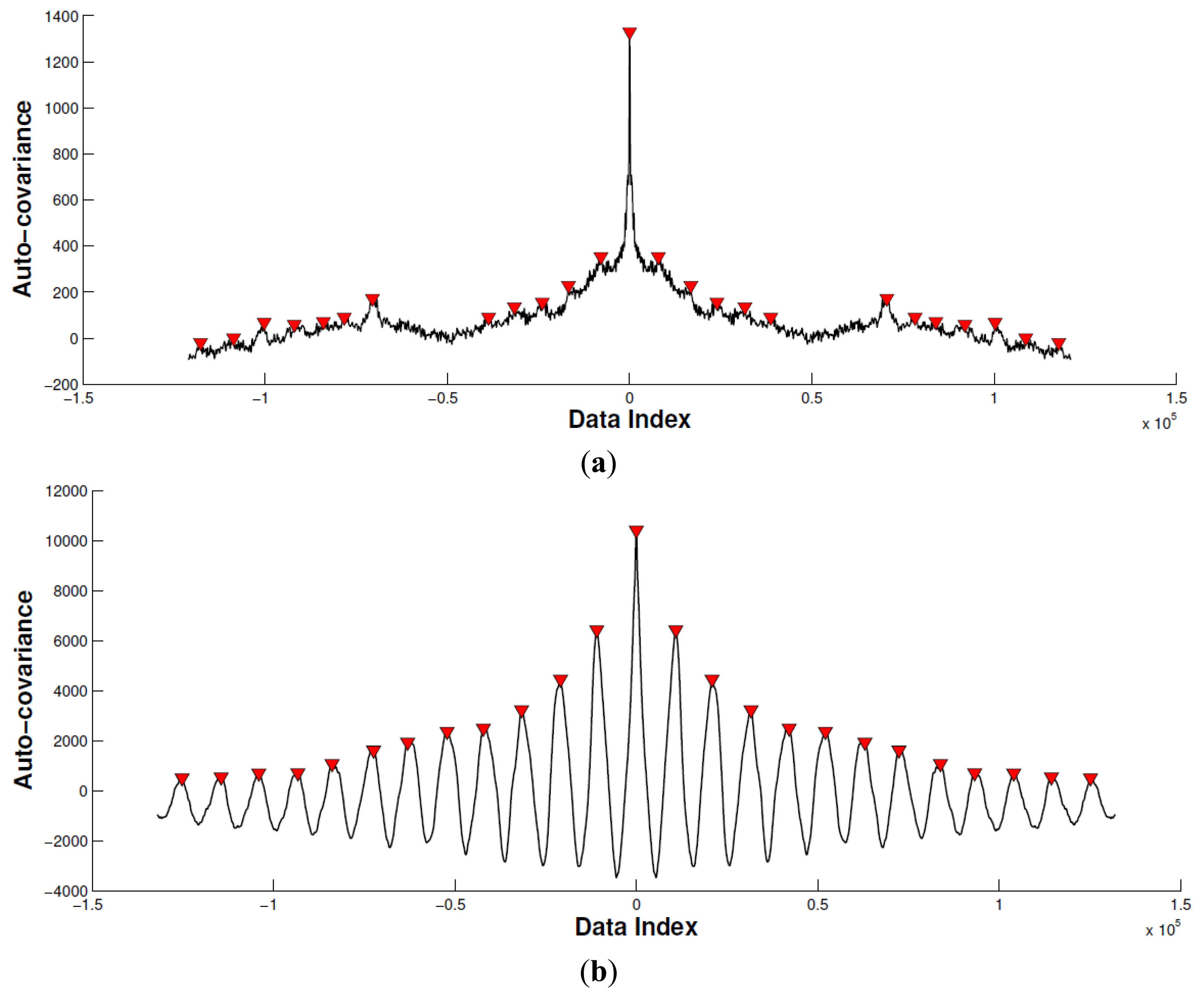
In this subsection, we calculate the cross-correlation to analyze the periodic property of the acceleration signal corresponding with biceps brachii (Figure 7). Specifically, we remove the mean of the acceleration signal before computing the cross-correlation. Then, we limit the maximum lag to 50% of the signal to achieve a good estimation of the cross-covariance.
By comparing the peak difference between the largest and second largest local peak with the predefined threshold ε, we determine if the movement is periodic. In this paper, the threshold ε is set as twice that of the second largest local peak value. As seen of in Figure 7, the horizontal axis indicates data index, and vertical axis indicates the auto-covariance result. The red triangle emphasizes the local peaks. According to the proposed method mentioned, Experiment 1 is recognized as a non-periodic movement, and Experiment 2 is recognized as a periodic movement. Based on this, the sEMG signal in Experiment 2 is segmented and connected as a new sEMG signal for the mean frequency calculation.
6.3. Mean Frequency Trend
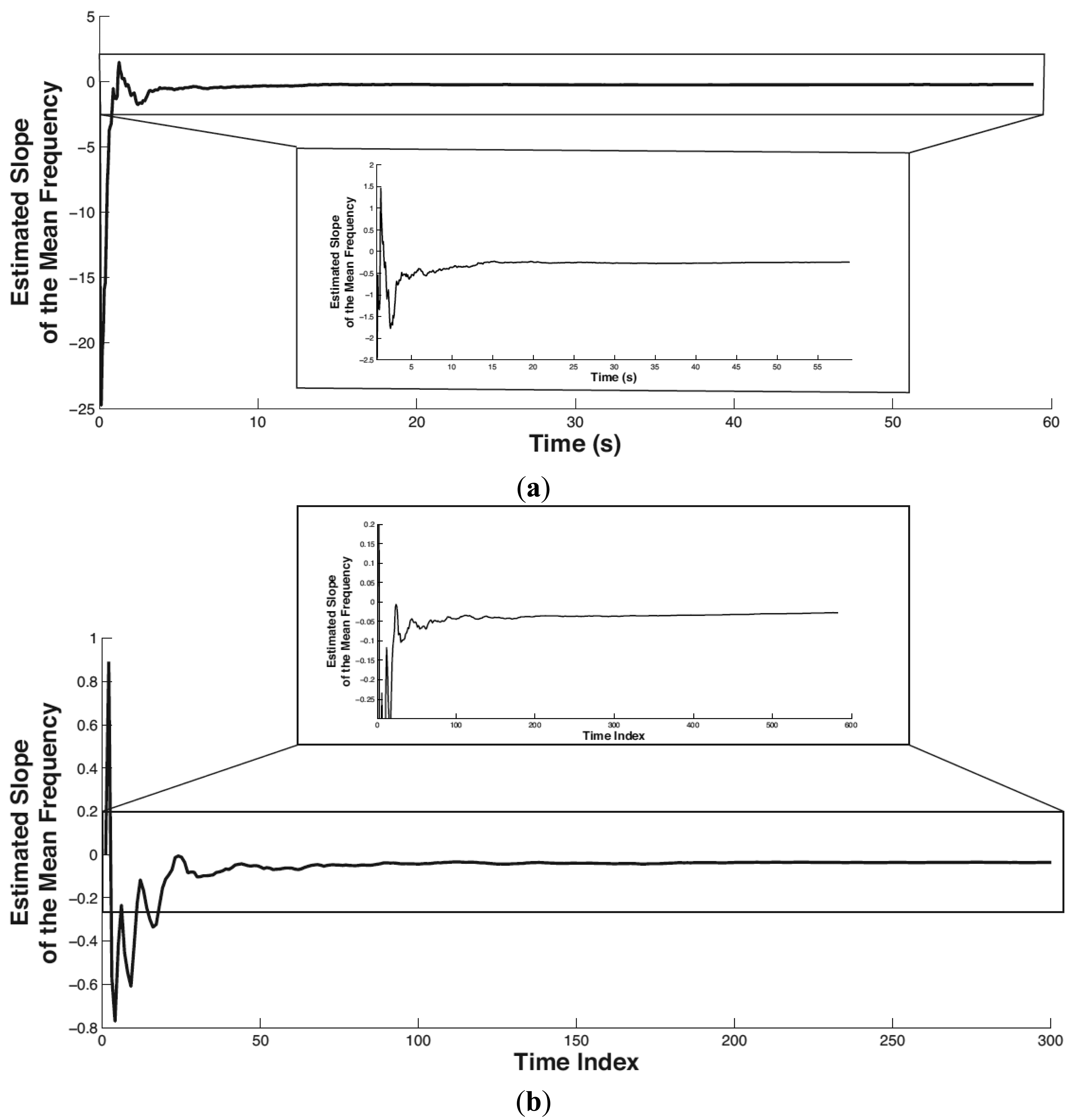
In this paper, the setting of the forgetting factor is λ = 0.95, which means the previous localized muscular fatigue level information is partially used in calculating the current muscular fatigue level. The initial value of φ̂t and pt is φ̂t(0) = 0, pt(0) = 10,000. The tracked trend of the mean frequency of biceps brachii is shown in Figure 8 where (a) and (b) correspond to Experiment 1 and Experiment 2, respectively. In both subplots, the partial view of the mean frequency trend shown below is plotted by limiting the x-scale. The horizontal axis denotes time in seconds (or time index). The vertical axis denotes the tracked slope (i.e., trend) of the mean frequency.
It is easy to see that the proposed method stabilizes in tracking the mean frequency trend within the initial 5 s. The slope of the mean frequency variance in Experiments 1 and 2 converges to −0.247 and −0.027, respectively. Both the slopes in Experiments 1 and 2 are negative, which is consistent with the scenario of physical fatigue. As the magnitude of time (in Experiment 1) is smaller than the time index (in Experiment 2) on the order of 10, correspondingly, the amount of the tracked slope in Experiment 1 is larger than that in Experiment 2 on the order of 10.
6.4. Localized and Overall Fatigue Levels
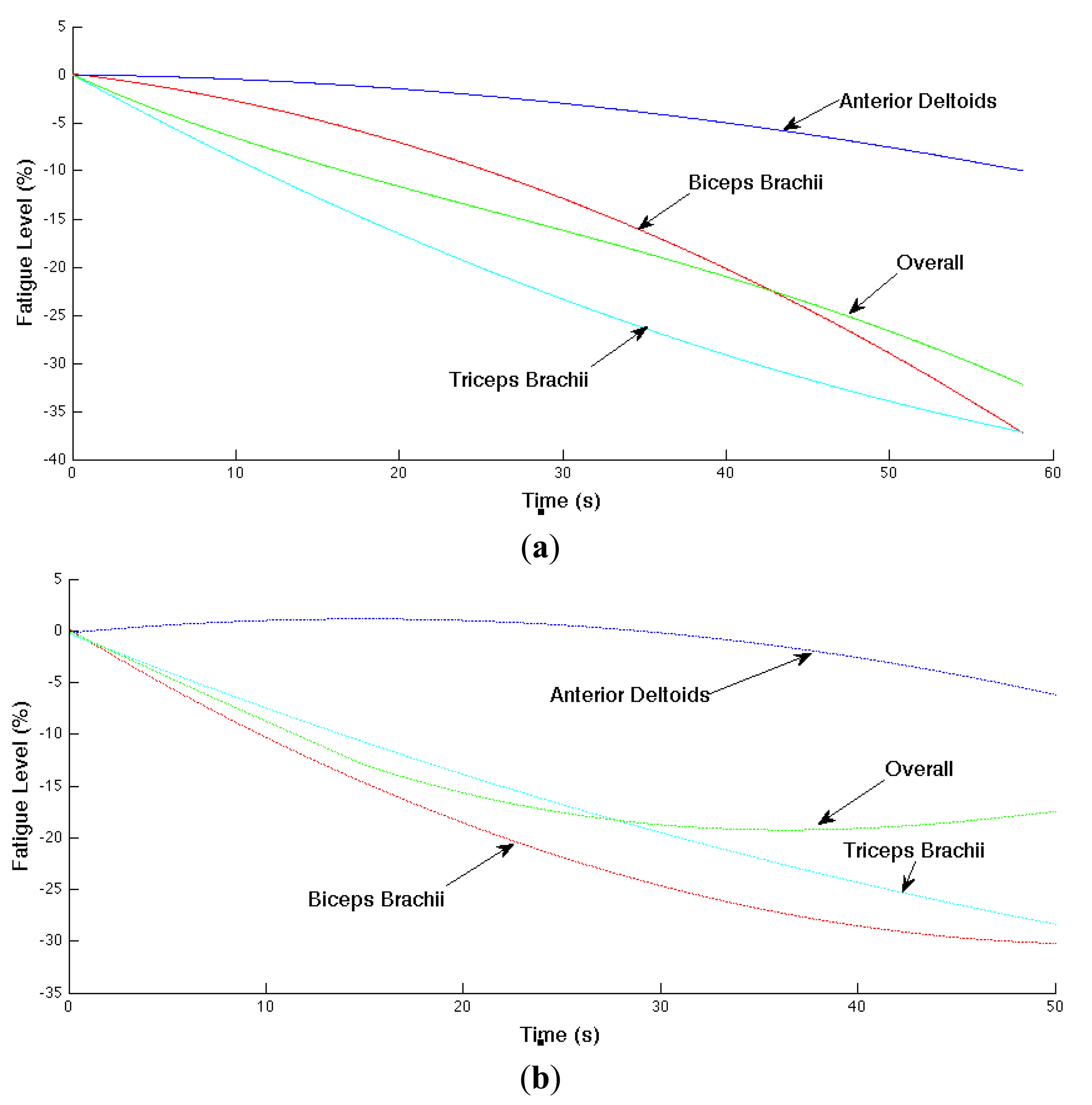
The localized muscular fatigue level is updated based on the mean frequency trend (i.e., estimated slope parameter of the mean frequency). In addition, we smoothed the computed fatigue level for better result visualization. The muscular and overall fatigue level trajectories are shown in Figure 9 where (a) and (b) correspond the computed overall fatigue level and corresponding localized muscular fatigue levels in Experiments 1 and 2, respectively. The horizontal axis is time (or time index) and vertical axis is the computed fatigue level in negative percentages.
In Experiment 1 (shown in (a)), the localized muscular fatigue level of the biceps brachii, anterior deltoids and triceps brachiii starts from 0%, indicating a non-fatigue status, and decreases gradually to −37%, −9% and −37%, indicating a fatigue status, whereas the overall fatigue level provides a compromise of the localized muscular fatigue levels starting from 0% to −32%. Similarly, in Experiment 2 (shown in (b)), the localized fatigue level of the biceps brachii, anterior deltoids, triceps brachii and the overall fatigue level starts from 0%, decreases to −30%, −6%, −28%, −17%, respectively.
6.5. System Validation
The developed fatigue-tracking system was evaluated with two experiments involving 17 subjects (male group: 10 subjects; female group: 7 subjects). The detailed experiment setting was explained in Section 2.3. The subjects were quite diverse, originating from 11 countries. According to the BMI classification, the subject group covered underweight, normal weight, overweight and obesity categories.
The statistics of the fatigue levels is given in Table 2. In both experiments, the localized fatigue levels (corresponding with biceps brachii, anterior deltoids and triceps brachii) and overall fatigue level at the end of the experiments are listed. As the designed experiments targeted at monitoring fatigue scenario, all the fatigue levels are negative, which is consistent with the observed muscle-shaking scenario. Confirmed by the feedback from the subjects after the experiments, we approximately conclude that the more tired the subject feels, the bigger the overall fatigue level is. Besides, as seen in Table 2, the fatigue levels differ between subjects. However, if the subject had a relatively higher overall fatigue level in Experiment 1, he/she always had a relatively higher overall fatigue level in Experiment 2, correspondingly.
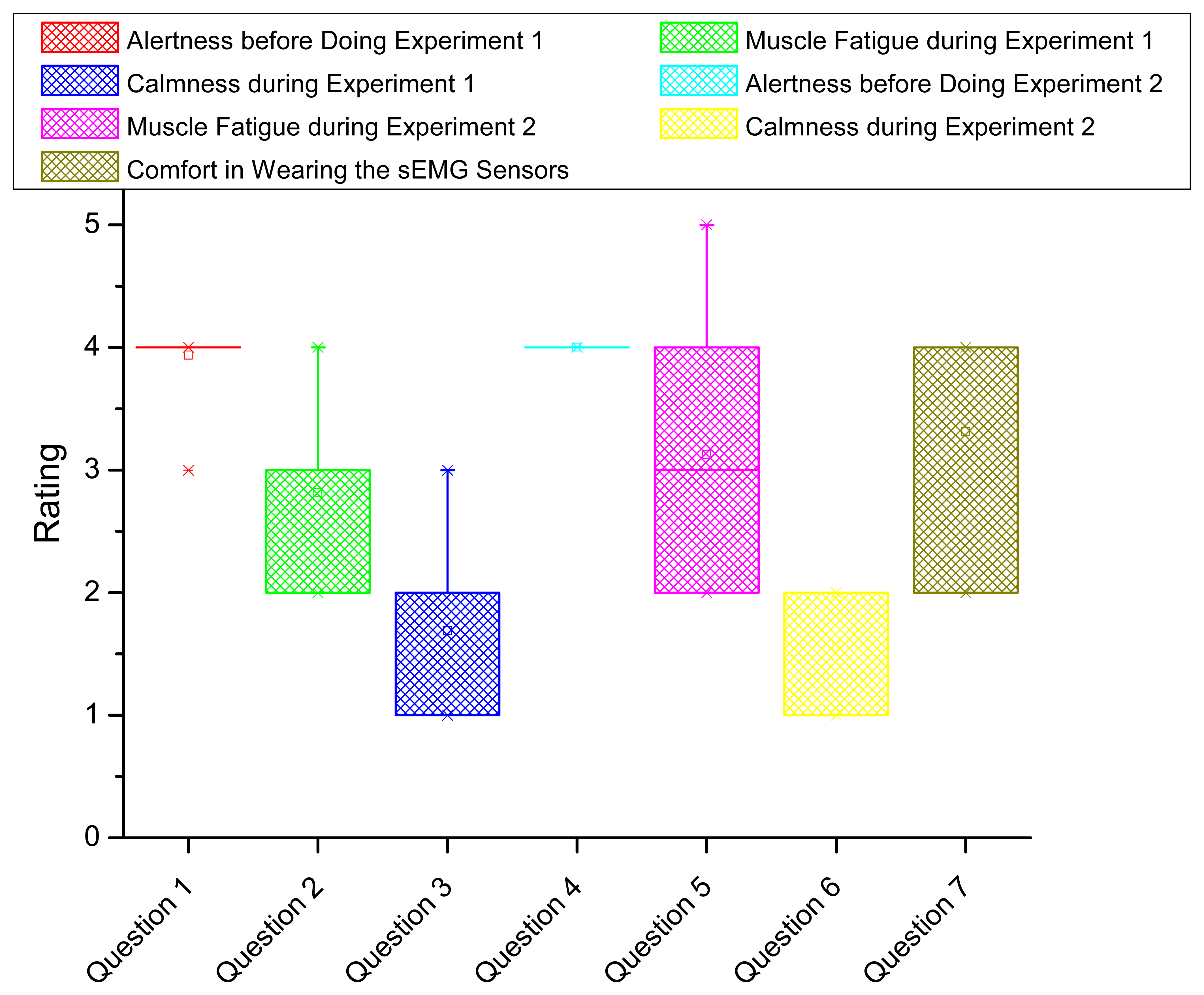
To evaluate the system from users' experience, we conducted a survey including seven questions as shown in Table 3. The questions cover the alertness, muscle fatigue feeling, calmness and comfort in both experiments. The rating starts from 1 to 5 corresponding with the least to the most intensity. Each subject is asked to complete the survey after the experiments.
The statistics of survey results is shown by box plot in Figure 10. The horizontal axis indicates the question index. The vertical axis shows the rating statistics. For each box (corresponding with one question), the upper and lower boundary represents the 25% and 75% of the interquartile range. The line and small square in the middle of the box indicates the median and mean value of the rating, respectively. Two small crosses locating above and below the box show the boundary of 1% and 99% of the rating values in the whole range. In Figure 10, we conclude the following results. First, nearly all the subjects are fully awake and alert before doing the experiments (from Questions 1 and 4), meaning their physiological status is proper for doing fatigue experiments. Second, during the fatigue experiments, the subjects averagely feel moderate fatigue whereas some of the subjects feel extreme fatigue in Experiment 1 and feel the worst fatigue in Experiment 2. All the subjects marked at least mild fatigue according to his/her feeling, which is consistent with the negative fatigue levels in Table 2. Overall, the subjects feel more fatigue in Experiment 2 compared in Experiment 1 (from Questions 2 and 5). Third, we compare the fatigue intensity change in Experiments 1 and 2 between the computed overall fatigue level and the subject's feeling where 73% coincidence is confirmed. Fourth, during the fatigue experiments, the subjects are in the condition between calm and slightly anxious (from Questions 3 and 6). Fifth, generally, the subjects feel the proposed fatigue-tracking system is acceptable in comfort (between moderately comfortable and very comfortable in Question 7).
7. Conclusions and Future Work
In this paper, we developed a wearable wireless system for tracking the status of fatigue in human movement. The proposed system is based on scientific electromyography and kinesiology studies, which show that the mean frequency decreases with the increase of the fatigue intensity. According to previous work, we assume that the decrease of mean frequency satisfies a linear relation with working time of a muscle under fatigue. We then used a rigorous statistical analysis to prove this assumption, upon which the definition of localized muscular fatigue level is based on. We then tracked the localized muscular fatigue levels by updating the parameters with the most current measurements by considering the fatigue process as a dynamic process. Furthermore, the overall fatigue level corresponding to a human movement was computed by fusing different localized muscular fatigue levels together. Finally, the developed fatigue tracking system was tested and verified with two fatigue experiments involving 17 subjects. In the proposed method, the setting of the “forgetting factor” and fatigue level fusion coefficient might vary according to different muscle types and practical applications. This could be a limitation to the application of our method. Nonetheless, our future work is to clarify this parameter setting issue.
Conflict of Interest
The authors declare no conflict of interest.
References
- Ji, Q.; Lan, P.; Looney, C. A probabilistic framework for modeling and real-time monitoring human fatigue. IEEE Trans. Syst. Man Cybern. 2006, 36, 862–875. [Google Scholar]
- Ma, R.; Chablat, D.; Bennis, F.; Ma, L. Human Muscle Fatigue Model in Dynamic Motions. In Latest Advances in Robot Kinematics; Springer: Dordrecht, The Netherland, 2012; pp. 349–356. [Google Scholar]
- Al-Mulla, M.; Sepulveda, F.; Colley, M. An autonomous wearable system for predicting and detecting localised muscle fatigue. Sensors 2011, 11, 1542–1557. [Google Scholar]
- Knaflitz, M.; Molinari, F. Assessment of muscle fatigue during biking. IEEE Trans. Neural Syst. Rehabil. Eng. 2003, 11, 17–23. [Google Scholar]
- Lamberts, R.; Swart, J.; Capostagno, B.; Noakes, T.; Lambert, M. Heart rate recovery as a guide to monitor fatigue and predic changes in performance parameters. Scand. J. Med. Sci. Sports 2010, 20, 449–457. [Google Scholar]
- Debold, E. Recent insights into muscle fatigue at the cross-bridge level. Front Physiol. 2012, 3, 1–14. [Google Scholar]
- Fitts, R. The cross-bridge cycle and skeletal muscle fatigue. J. Appl. Physiol. 2008, 104, 551–558. [Google Scholar]
- Komura, T.; Shinagawa, Y.; Kunii, T. Creating and retargetting motion by the musculoskeletal human body model. Vis. Comput. 2000, 16, 254–270. [Google Scholar]
- Karatzaferi, C.; Chase, P. Muscle fatigue and muscle weakness: What we know and what we wish we did. Front Physiol. 2013, 4, 1–3. [Google Scholar]
- Tang, C.; Stojanovic, B.; Tsui, C.; Kojic, M. Modeling of muscle fatigue using Hill's model. Bio-Med. Mater. Eng. 2005, 15, 341–348. [Google Scholar]
- Potes, C. Assessment of Human Muscle Fatigue from Surface EMG Signals Recorded during Isometric Voluntary Contractions. Proceedings of 25th Southern Biomedical Engineering Conference, Miami, FL, USA, 15–17 May 2009; pp. 267–270.
- Chang, K.; Liu, S.; Wu, X. A wireless sEMG recording system and its application to muscle fatigue detection. Sensors 2012, 12, 489–499. [Google Scholar]
- Spulber, I.; Georgiou, P.; Eftekhar, A.; Toumazou, C.; Duffell, L.; Bergmann, J.; Mcgregor, A.; Mehta, T.; Hernandez, M.; Burdett, A. Frequency Analysis of Wireless Accelerometer and EMG Sensors Data: Towards Discrimination of Normal and Asymmetric Walking Pattern. Proceedings of IEEE International Symposium on Circuits and Systems, Seoul, Korea, 20–23 May 2012; pp. 2645–2648.
- Dayan, O.; Spulber, I.; Eftekhar, A.; Georgiou, P.; Bergmann, J.; Mcgregor, A. Applying EMG Spike and Peak Counting for a Real-Time Muscle Fatigue Monitoring System. Proceedings of IEEE Biomedical Circuits and Systems Conference, Hsinchu, Taiwan, 28–30 November 2012; pp. 41–44.
- Lucev, Z.; Krois, I.; Cifrek, M. Application of Wireless Intrabody Communication System to Muscle Fatigue Monitoring. Proceedings of IEEE Instrumentation and Measurement Technology Conference , Austin, TX, USA, 3–6 May 2010; pp. 1624–1627.
- Cryer, J.; Chan, K. Time Series Analysis with Applications in R; Springer: New York, NY, USA, 2008. [Google Scholar]
- Al-Mulla, M.; Sepulveda, F.; Colley, M. A review of non-invasive techniques to detect and predict localised muscle fatigue. Sensors 2011, 11, 3545–3594. [Google Scholar]
- Ma, L.; Chablat, D.; Bennis, F.; Zhang, W.; Guillaume, F. A new muscle fatigue and recovery model and its ergonomics application in human simulation. Virtual Phys. Prototyp. 2010, 5, 123–137. [Google Scholar]
- Rechy-Ramirez, E.; Hu, H. Stages for Developing Control Systems Using EMG and EEG Signals: A Survey; Technical Report; University of Essex: Colchester, UK, 2011. [Google Scholar]
- Santiago, I. Joint-Level Fatigue Simulation for Its Exploitation in Human Posture Characterization and Optimization. MS.c. Thesis, University of Alcala, Madrid, Spain, 2003. [Google Scholar]
- Slotine, J.; Li, W. Applied Nonlinear Control; Prentice Hall: Englewood Cliffs, NJ, USA, 1991. [Google Scholar]
- Dong, H.; Ugalde, I.; El Saddik, A. Development of a Fatigue-Tracking System for Monitoring Human Body Movement. Proceedings of IEEE Instrumentation and Measurement Technology Conference, Montevideo, Uruguay, 12–15 May 2014.
- Young, P. Recursive Estimation and Time-Series Analysis; Springer: Berlin, Germany, 2011. [Google Scholar]


| Subject | Gender Group | ||||||||||
|---|---|---|---|---|---|---|---|---|---|---|---|
| No. | m1 | m2 | m3 | m4 | m5 | m6 | m7 | m8 | m9 | m10 | |
| F | F | 296.625 | 677.604 | 59.511 | 18.423 | 8.032 | 205.884 | 57.706 | 659.796 | 17.993 | 482.152 |
| test | p | 0.000 | 0.000 | 0.000 | 0.000 | 0.005 | 0.000 | 0.000 | 0.000 | 0.000 | 0.000 |
| No. | f1 | f2 | f3 | f4 | f5 | f6 | f7 | ||||
| F | F | 968.508 | 40.212 | 4.174 | 438.636 | 523.176 | 134.794 | 1310.249 | |||
| test | p | 0.000 | 0.000 | 0.041 | 0.000 | 0.000 | 0.000 | 0.000 | |||
| Subject | No. | Fatigue Levels in Experiment 1 | Fatigue Levels in Experiment 2 | ||||||
|---|---|---|---|---|---|---|---|---|---|
| Biceps Brachii | Anterior Deltoids | Triceps Brachii | Overall | Biceps Brachii | Anterior Deltoids | Triceps Brachii | Overall | ||
| Male Group | m1 | −9% | −13% | −8% | −10% | −9% | −24% | −20% | −20% |
| m2 | −8% | −25% | −39% | −31% | −21% | -25% | −42% | −32% | |
| m3 | −21% | −19% | −31% | −25% | −8% | −19% | −28% | −22% | |
| m4 | −13% | −18% | −21% | −18% | −10% | −40% | −24% | −31% | |
| m5 | −14% | −6% | −15% | −13% | −16% | −15% | −27% | −21% | |
| m6 | −12% | −23% | −11% | −17% | −5% | −15% | −29% | −22% | |
| m7 | −14% | −21% | −15% | −17% | −10% | −17% | −56% | −42% | |
| m8 | −8% | −20% | −13% | −15% | −14% | −25% | −46% | −35% | |
| m9 | −11% | −11% | −13% | −12% | −14% | −11% | −36% | −26% | |
| m10 | −10% | −21% | −16% | −17% | −4% | −24% | −8% | −18% | |
| Female Group | f1 | −7% | −28% | −32% | −28% | −31% | −15% | −47% | −37% |
| f2 | −22% | −5% | −36% | −29% | −33% | −15% | −24% | −26% | |
| f3 | −37% | −9% | −37% | −32% | −30% | −6% | −28% | −17% | |
| f4 | −3% | −24% | −39% | −32% | −10% | −4% | −43% | −34% | |
| f5 | −14% | −28% | −14% | −21% | −13% | −19% | −14% | −16% | |
| f6 | −4% | −18% | −9% | −14% | −3% | −5% | −11% | −8% | |
| f7 | −10% | −39% | −16% | −29% | −12% | −5% | −35% | −27% | |
| Questions | 1 | 2 | 3 | 4 | 5 |
|---|---|---|---|---|---|
| Q1: Alertness before Doing Experiment 1 | Deeply asleep | Lightly asleep | Drowsy | Fully awake and alert | Hyper-alert |
| Q2: Muscle Fatigue Feeling during Experiment 1 | No fatigue | Mild fatigue | Moderate fatigue | Extreme fatigue | The worst fatigue |
| Q3: Calmness during Experiment 1 | Calm | Slightly anxious | Anxious | Very anxious | Panicky |
| Q4: Alertness before Doing Experiment 2 | Deeply asleep | Lightly asleep | Drowsy | Fully awake and alert | Hyper-alert |
| Q5: Muscle Fatigue Feeling during Experiment 2 | No fatigue | Mild fatigue | Moderate fatigue | Extreme fatigue | The worst fatigue |
| Q6: Calmness during Experiment 2 | Calm | Slightly anxious | Anxious | Very anxious | Panicky |
| Q7: Comfort in Wearing the Fatigue-Tracking System | Not comfortable at all | Mildly confortable | Moderately comfortable | Very comfortable | Extremely comfortable |
© 2014 by the authors; licensee MDPI, Basel, Switzerland. This article is an open access article distributed under the terms and conditions of the Creative Commons Attribution license ( http://creativecommons.org/licenses/by/3.0/).
Share and Cite
Dong, H.; Ugalde, I.; Figueroa, N.; El Saddik, A. Towards Whole Body Fatigue Assessment of Human Movement: A Fatigue-Tracking System Based on Combined sEMG and Accelerometer Signals. Sensors 2014, 14, 2052-2070. https://doi.org/10.3390/s140202052
Dong H, Ugalde I, Figueroa N, El Saddik A. Towards Whole Body Fatigue Assessment of Human Movement: A Fatigue-Tracking System Based on Combined sEMG and Accelerometer Signals. Sensors. 2014; 14(2):2052-2070. https://doi.org/10.3390/s140202052
Chicago/Turabian StyleDong, Haiwei, Izaskun Ugalde, Nadia Figueroa, and Abdulmotaleb El Saddik. 2014. "Towards Whole Body Fatigue Assessment of Human Movement: A Fatigue-Tracking System Based on Combined sEMG and Accelerometer Signals" Sensors 14, no. 2: 2052-2070. https://doi.org/10.3390/s140202052
APA StyleDong, H., Ugalde, I., Figueroa, N., & El Saddik, A. (2014). Towards Whole Body Fatigue Assessment of Human Movement: A Fatigue-Tracking System Based on Combined sEMG and Accelerometer Signals. Sensors, 14(2), 2052-2070. https://doi.org/10.3390/s140202052