A Kalman Filter Implementation for Precision Improvement in Low-Cost GPS Positioning of Tractors

 ,
,
Abstract
: Low-cost GPS receivers provide geodetic positioning information using the NMEA protocol, usually with eight digits for latitude and nine digits for longitude. When these geodetic coordinates are converted into Cartesian coordinates, the positions fit in a quantization grid of some decimeters in size, the dimensions of which vary depending on the point of the terrestrial surface. The aim of this study is to reduce the quantization errors of some low-cost GPS receivers by using a Kalman filter. Kinematic tractor model equations were employed to particularize the filter, which was tuned by applying Monte Carlo techniques to eighteen straight trajectories, to select the covariance matrices that produced the lowest Root Mean Square Error in these trajectories. Filter performance was tested by using straight tractor paths, which were either simulated or real trajectories acquired by a GPS receiver. The results show that the filter can reduce the quantization error in distance by around 43%. Moreover, it reduces the standard deviation of the heading by 75%. Data suggest that the proposed filter can satisfactorily preprocess the low-cost GPS receiver data when used in an assistance guidance GPS system for tractors. It could also be useful to smooth tractor GPS trajectories that are sharpened when the tractor moves over rough terrain.1. Introduction
Global Positioning Systems (GPS) are nowadays used in many agricultural tasks [1–3]. GPS receivers with RTK differential corrections are frequently employed in agricultural equipment [4,5]. Nevertheless, tasks such as yield mapping [6] and assisted guidance in cereal fertilization do not always need centimeter precision. In consequence, some companies manufacture assisted guidance systems for tractors equipped with low-cost GPS receivers, such as Agroguia® [7] and Tractordrive® [8], for example, in Spain. Moreover, the universalization of mobile computing with smartphones and tablet devices, equipped with powerful processors and low-cost embedded GPS receivers, makes the use of these devices in agricultural tasks attractive. However, due to a quantization effect, most low-cost GPS receivers provide positions on a rectangular grid of some decimeters on each side. Because of this fact, low speed trajectories and parts of the trajectories with headings close to a coordinate axle suffer from significant speed, position, and heading errors when using low-cost GPS receivers.
The aim of this work is to smooth the tractor trajectories acquired by low-cost GPS receivers, by improving the precision of their position data by decreasing their quantization error. To do so, an implementation of the Kalman filter was applied to the trajectory data provided by a low-cost GPS receiver that was placed on a farm tractor.
The following points are introduced below for a better understanding of this implementation: (i) error considerations for GPS receivers; (ii) the quantization effects in low-cost GPS receivers; (iii) the kinematic model of a tractor; (iv) the Kalman filter; and (v) the Kalman filter tuning.
1.1. Error Considerations for GPS Receivers
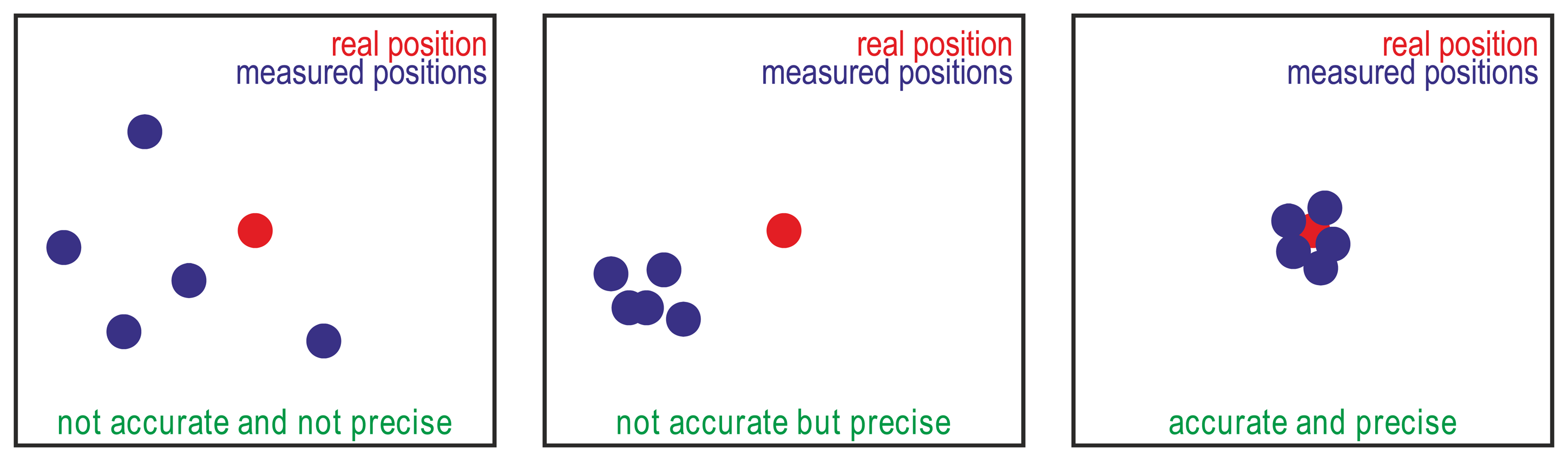
Two kinds of errors can be defined for GPS receivers and GPS guidance systems [9–11]: (i) precision, relative accuracy, reproducibility, repeatability, or pass-to-pass accuracy, which refer to the degree to which the measurements reported by a GPS receiver in a fixed placement provide close positions regardless of the real position; and (ii) accuracy or absolute accuracy, which refer to the degree of closeness of the measured positions to their real position. Figure 1 illustrates the difference between precision and accuracy.
In guidance system applications, where the time between each pass is relatively short and the trajectories are not saved from year to year, precision can be considered the most important variable. In this way, low-cost GPS receivers with 10 m accuracy but sub-meter precision will be alternatives in such agricultural task.
1.2. Quantization Effects in Low-Cost GPS Receivers
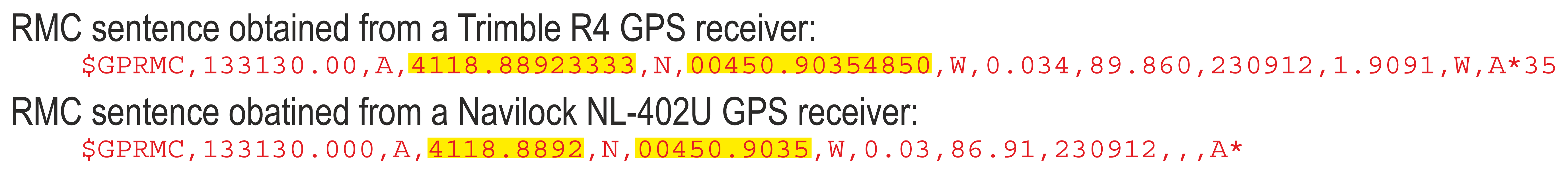
The most common chipsets that low-cost GPS receivers and embedded mobile computing devices integrate are the Sirf [12], the U-blox [13], and the MTK [14]. Receivers with either of these chipsets transmit positioning information by means of the National Marine American Association (NMEA) 0183 protocol, and provide latitude and longitude geodetic coordinates with usually only eight digits for latitude and nine for longitude (Figure 2).
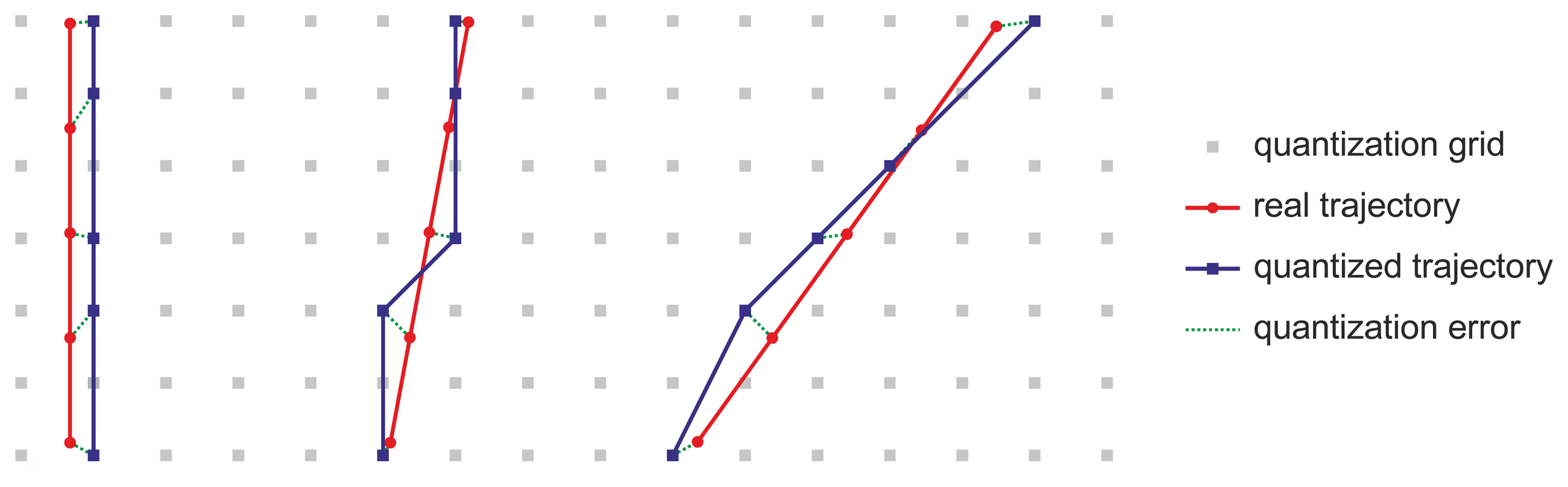
Geodetic coordinates are not appropriate for agricultural data processing and are usually converted to Cartesian coordinates. When positions in geodetic coordinates with a quantization of only 8 digits for latitude and 9 for longitude are converted to Cartesian coordinates such as Universal Transverse Mercator (UTM) [15–17] or East, North, Up (ENU) [18], they appear on a rectangular grid of some decimeters in size. Specifically, at the place where the real tests were conducted, with a latitude of 41.32° N and a longitude of 4.84° W, the quantization grid is 14 cm and 18 cm on the X and Y axes, respectively, in UTM coordinates. Position, speed, and heading errors appear in the trajectories on this grid, which provoke oscillations in the trajectory of the tractor. These oscillations are especially noticeable when they are acquired at low speeds and with headings close to the direction of a coordinate axis (Figure 3).
On the basis of their professional experience with Agroguia® [7] and Tractordrive® [8], the authors state that these oscillations negatively affect the use of low-cost GPS receivers in GPS assisted-guidance systems for tractors.
1.3. Kinematic Model of a Tractor
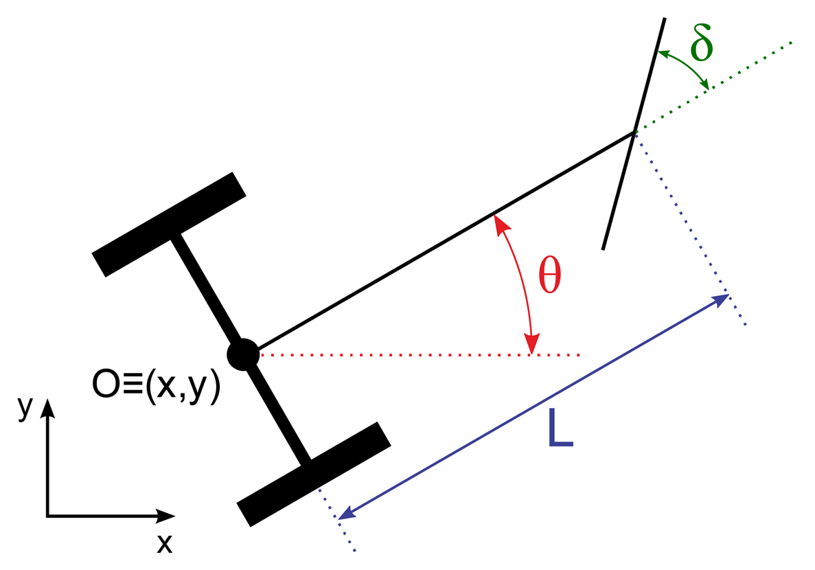
A classic tractor has two front wheels that steer as well as two rear wheels that are straight-driven. The behavior of this kind of tractor vehicle is typically modeled following the tricycle vehicle model [19]. In this model, the system inputs are the vehicle speed modulus, u, and the front-wheel steering angle, δ. The tractor behavior can be described with a vector state, q, defined by the expression:
1.4. The Kalman Filter
The Kalman filter is an efficient, recursive, mathematical algorithm that processes, at each step, inaccurate observation input data and generates a statistically optimal estimate of the subjacent real system state, by employing a prediction model and an observation model [20].
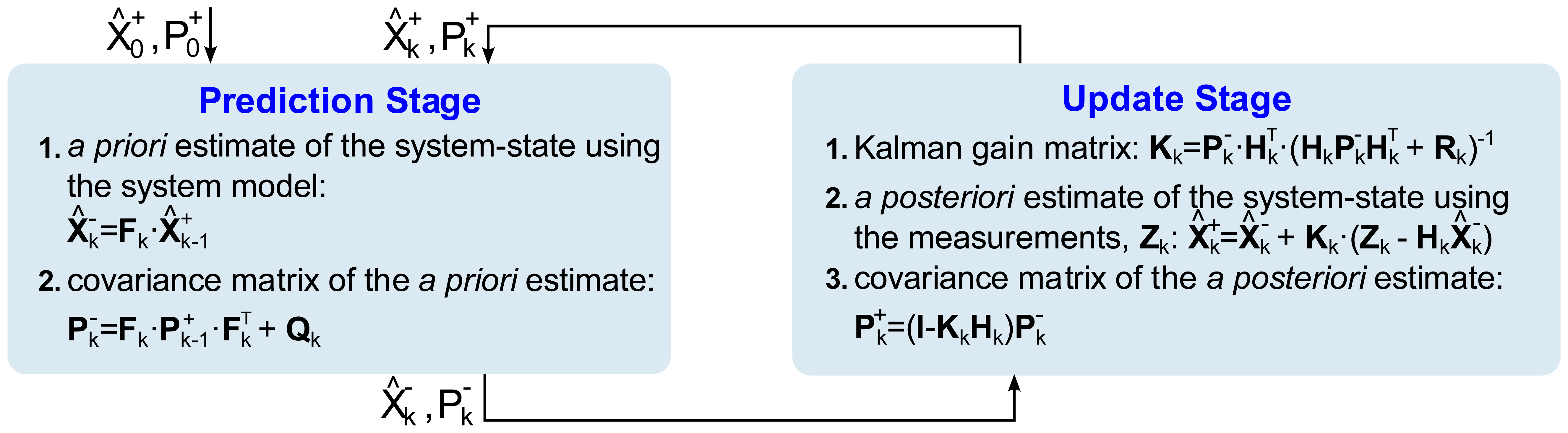
The basic functioning of the filter is conceptualized into two stages. The first stage is called the prediction stage, as it produces an a priori system state estimate from the previous state, by using a system evolution prediction model. The second stage, known as the update stage, takes into account measurements in the system to produce an a posteriori state estimate, by correcting the previous a priori estimate. This two-stage process starts with an initial estimated state, , and is repeated in a loop recursively until filtering ends (Figure 5).
Figure 5 summarizes the steps in each stage of the Kalman filtering process and it presents the matrices that are involved and the steps followed to implement the Kalman filter [20,21]. Fk is the state transition model matrix, which performs the prediction model. Hk is the observation model matrix, which maps the state vector space into the measurements vector space. is the a priori state estimate vector, resulting from the prediction stage. is the a posteriori state estimate vector, derived from the measurements update stage. zk is the measurements vector obtained from the system sensors. Kk is the optimal Kalman gain matrix, which weights the importance of the innovation that introduces the measurements vector zk in the update stage. is the a priori state covariance matrix, which provides the a priori estimation error covariance after the prediction stage. is the a posteriori state covariance matrix, containing the a posteriori estimation error covariance, given after the update stage. Q is the process noise covariance matrix of the prediction stage noise, which somehow ponders the weight of the process estimates. R is the observation noise covariance matrix of the update stage noise, which in a way ponders the degree of confidence in each one of the measurements. The relative weights become greater as the covariance matrix elements become smaller, meaning that the quantities involved are increasingly reliable.
1.5. The Tuning of the Kalman Filter
Kalman filter tuning consists of setting the relevant parameter values for the related noise covariance matrices Q, R, and [22]. Matrices Q, R, , and reflect, respectively, the certainty or accuracy of the prediction model, the measurement model, the a priori prediction, and the a posteriori correction. The Kalman filter uses these matrices to weight the relevance and degree of confidence in predictions and measurements. The Kalman filter assumes that the involved noise characteristics have a zero-mean multivariate Gaussian distribution with covariance matrices Q and R for the process and measurements noises, respectively. Process noise is the random vector affecting the state xk, meanwhile measurement noise is the random vector affecting the measurements vector xk. Typically Q and R values must be estimated, in order to achieve statistically optimal filtering results. A covariance matrix contains the variance and cross-covariance information between each pair of elements of a random vector. In a general case, given a random vector, Y=[Y1Y2…Yn]T, its covariance matrix is expressed as:
There are two main approaches to address the filter tuning: static and dynamic. Static tuning approaches only tune the filter just before its use. Static procedures are based on techniques such as the Autocovariance Least Squares (ALS) method [24], performance-convergence cost functions [25], and general numerical optimization methods [26]. On the other hand, dynamic or adaptive tuning approaches tune the filter while it is operating, thus providing a self-tuning capability. Dynamic tuning methods are based on techniques such as Fuzzy Logic (FL) [27], Artificial Neural Networks (ANN) [28], Reinforcement Learning (RL) [29], the Dynamic Error System Analysis (DESA) method [30], and Genetic Algorithms (GA) [31,32]. Adaptive methods tend to yield a more robust behavior in cases such as those where noise characteristics change in time.
2. Method
This section comprises the work carried out in this survey. Section 2.1 outlines the particularization of the Kalman filter along with the prediction model that is employed. Section 2.2 deals with the method employed to tune the filter, in order to achieve a suitable performance with artificial data. Section 2.3 explains the experimental system employed in real field tests, to check the behavior of the proposed system.
2.1. Kalman Filter Particularization in Tractor Guidance
The system presented in this study uses a particularization of the Kalman filter applied to GPS receiver data, in order to achieve path smoothing and partial restoration of the lost resolution in positioning data. The prediction model of this system is based on the tricycle kinematic model, seen in Equation (2), assuming that the vehicle speed and heading angle will change slowly. Additionally, the system also makes use of the measurements provided by a GPS receiver to update the predictions previously made.
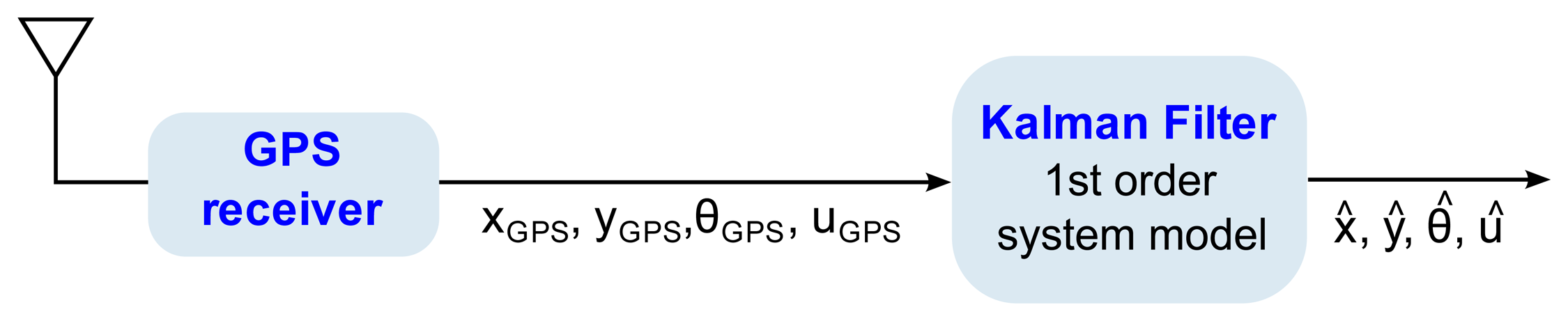
The system takes the array of GPS measurements zk(xGPS, YGPS, θGPS,uGPS)T, as input variables, where xGPS is the position in the X-axis, yGPS is the position in the Y-axis, θGPS is the measured heading angle formed by the tractor heading and the positive X-semiaxis, and uGPS is the speed modulus of the tractor. Given these inputs, zk, to the system, a related system state-vector is defined as xk = (xk,yk, θk,uk)T, which will be estimated by the Kalman filter. Figure 6 shows a black box diagram of this particular Kalman filter implementation.
Based on the system state, xk, along with Equation (2), a prediction model is applied, which supposes that vehicle heading angle (θ) and speed (u) will change slowly. The a priori state estimate is obtained from the previous a posteriori state estimate as:
Labeling the a priori state estimate vector as and the a posteriori state estimate vector as , Equations (4)–(7) are rewritten into the matrix form of the Kalman filter as:
It may be seen from Equation (9) that the prediction matrix has to be updated at every step, since the variable can change within each iteration, and the prediction matrix Fk depends on it in a non-linear way, which is not accounted for in the Fk matrix.
It is necessary to define the observation model matrix, Hk, in Equation (10), for the complete characterization of the proposed Kalman filter instance:
As the system state vector and measured magnitudes perfectly match, the particular observation model matrix Hk is chosen as the identity matrix in Equation (11):
2.2. Procedures
The Kalman filter was particularized for tractor guidance as detailed in Section 2.1, and the F and H system model matrices were obtained. Assuming statistical independence between all state variables, and assuming that the covariance matrices are time-invariant, the Q and R covariance matrices can be represented as Equation (12):
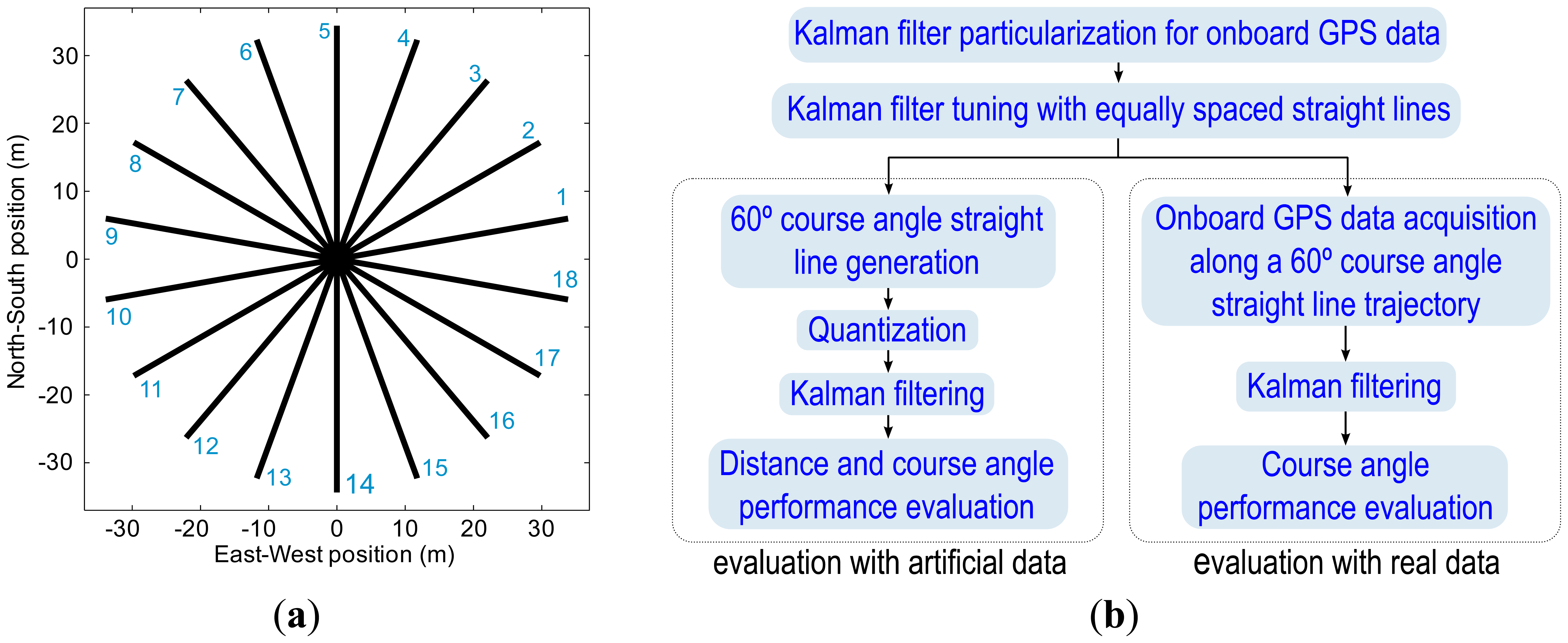
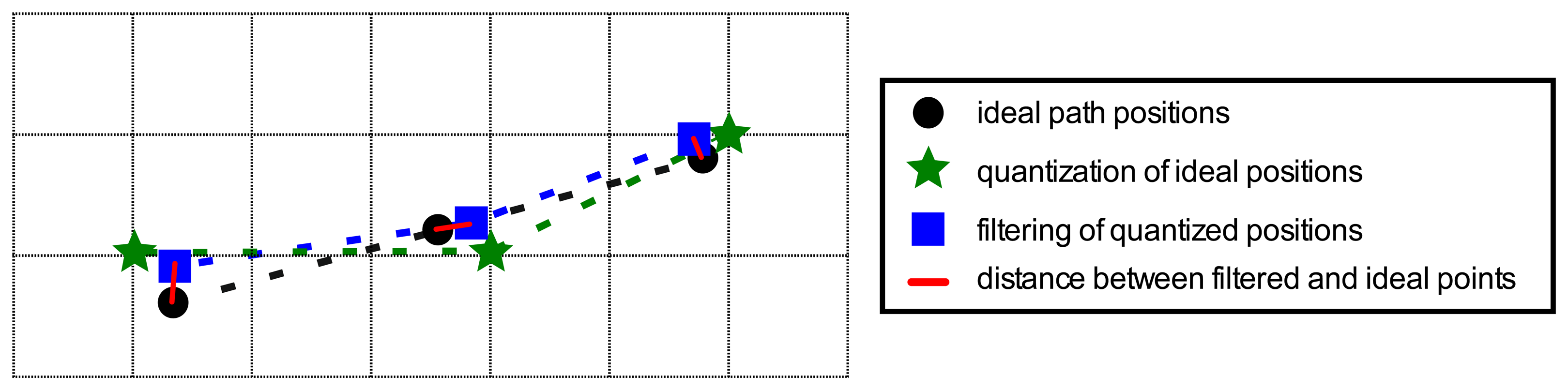
The Kalman filter was tuned using Monte Carlo Sampling techniques [33], by repeating the following two steps two million times. Initially, the elements of covariance matrices Q and R were randomly chosen between 0 and 6. Secondly, the particularized Kalman filter, using these covariance matrices, was applied over the 18 straight lines in Figure 7a, and then the Root Mean Square Error (RMSE) was computed, following Equation (13), over all straight lines, in which N is the number of samples, x̂i the i-th estimate of the X axis position, ŷi the i-th estimate of the Y axis position, and x and y are the ideal position reference coordinates. The couple of matrices with the lowest Root Mean Square Error were taken as covariance matrices Q and R. Figure 8 and Equation (13) detail the Root Mean Square Error (RMSE) computing procedure.
The proposed Kalman filter performance was evaluated with artificial data, through the following steps (Figure 7b): (i) a set of 18 ideal straight trajectories (Figure 7a) were sampled at a 5 Hz update rate, following vehicle kinematics constraints, at a constant speed of 5 km/h, which is a typical speed for agricultural tasks; (ii) trajectories were quantized to a 14 × 18 cm grid, because in Valladolid, Spain, when low-cost GPS receivers that provide eight digits for latitude and nine for longitude in NMEA are employed, positions appears over this grid; (iii) the proposed Kalman filter model was applied to the quantized paths; and (iv) the performance improvements were evaluated in terms of distance with respect the ideal path using all the paths shown in Figure 7a, and in terms of course angle distribution by using a 60° heading angle straight path.
Finally, the proposed Kalman filter performance was evaluated with real GPS data by following the next steps (Figure 7b): (i) GPS receiver data were acquired at a 5 Hz update rate from a GPS placed on a tractor that traveled along straight path with a 60° heading angle, and the GPS positions were converted to UTM coordinates; (ii) the proposed Kalman filter was applied to the acquired data; and (iii) the performance achievements in course angle distribution were evaluated. All the required simulations and data processing were carried out in MATLAB® programming environment.
2.3. Experimental System
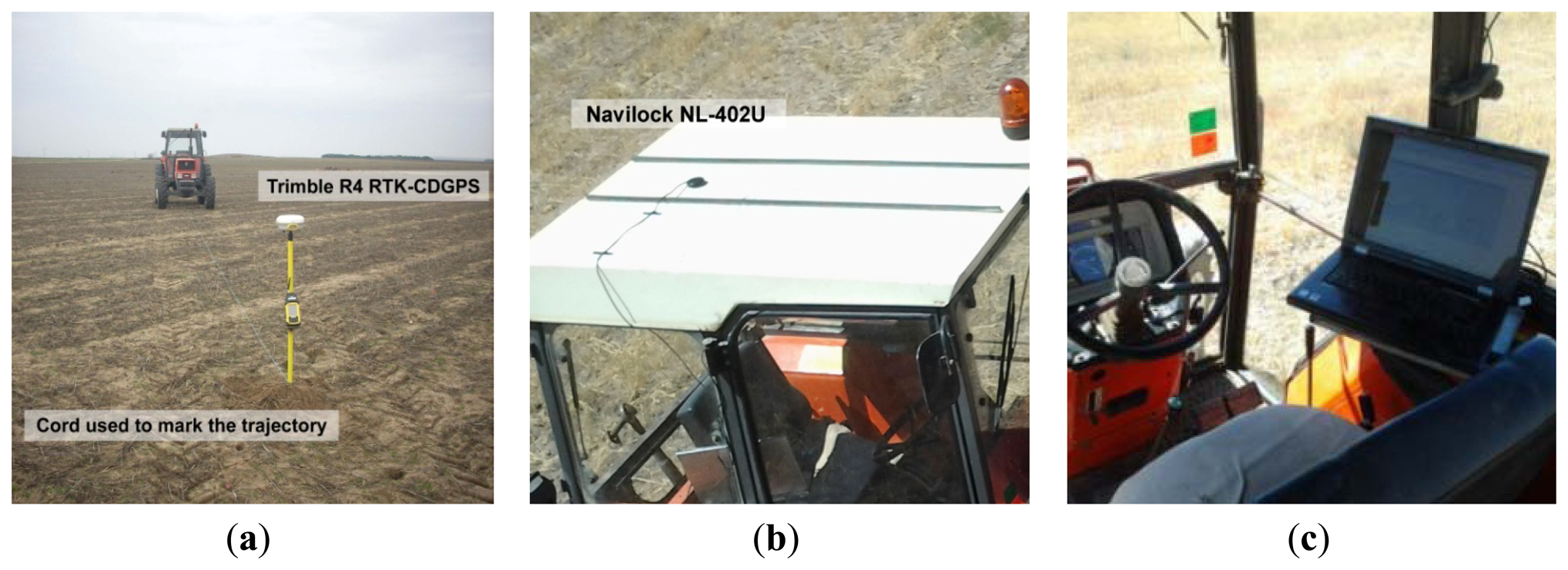
The materials employed in the experimental tests of this article were: a low-cost GPS receiver, a precise GPS receiver, a laptop computer, and an agricultural tractor. The low-cost GPS receiver was a Navilock NL-402U with an U-blox LEA-5H chipset (Figure 9b), and it was employed to acquire the GPS trajectories to be processed in this article at a 5 Hz rate. A precise Trimble R4 GPS receiver, configured to use RTK corrections, was employed to position the stakes that were used to mark the paths in the plot (Figure 9a). The laptop was a Lenovo N3000 (Figure 9c) and it was used to acquire and store the trajectories from the low-cost GPS receiver. The agricultural tractor was a Kubota M6950DT (Figure 9a), and it was employed to perform the trajectories with the low-cost GPS receiver over its cab (Figure 9b).
Each one of the straight trajectories of the experimental tests was marked with three stakes and were joined by a cord. The stakes were driven into the center of the trajectory and at each extreme. Figure 9a shows one of the trajectories and one stake.
GPS receiver data were read and processed with an application running on the laptop. The application, developed using Labwindows CVI, read the NMEA sentences from the GPS receiver and transformed the geodetic data of the NMEA sentences to UTM Cartesian coordinates for analysis.
3. Results
The tuning results, following the method presented in Section 2.2, were obtained using: (i) the artificially generated paths (Figure 7a) with a constant speed of 5 km/h; (ii) a 14 × 18 cm resolution quantization grid; (iii) an update rate of 5 Hz; (iv) the Kalman filtering model proposed in Section 2.1; and (v) the Root Mean Square Error minimizing criterion, defined in Section 2.2. The process noise covariance matrix, the measurements noise covariance matrix, and the a posteriori state covariance matrix were as follows:
These matrices, Equation (14), resulting from Kalman filter tuning, were used for both the simulations with artificial data and the real experimental data obtained from the onboard GPS receiver.
Simulations and real tests were executed to evaluate the Kalman filter performance. As Figure 10 visually illustrates, significant trajectory smoothing and resolution restoration achievements were accomplished in both situations, and no delays are noticed in either simulations or real tests. The achievements are shown along a selected path with a 60° heading angle, for both an artificially generated straight line path and onboard GPS receiver real data.
The properties and improvements of this proposed method are shown with the distance errors histogram (Figure 11), the RMSE and the 95th-percentile of the distance errors (Table 1), and the heading angle histogram (Figure 12).
Figure 11 presents the distance error histogram with regard to real reference positions, before and after filtering. These histograms were generated with the data from all the paths in Figure 7a. It is observed that, before applying the proposed Kalman filter, there are distance errors of up to 10 cm whereas, after applying the Kalman filter, the distance errors go no higher than 6 cm (Figure 11).
The RMSE and the 95th-percentile were computed, on the basis of the statistical distribution of the distance errors, as shown in Figure 11. These measurements can be employed to quantify the error improvement achieved by the proposed filtering. Table 1 refers to the RMSE of the quantization error, which was reduced by 42.98%.
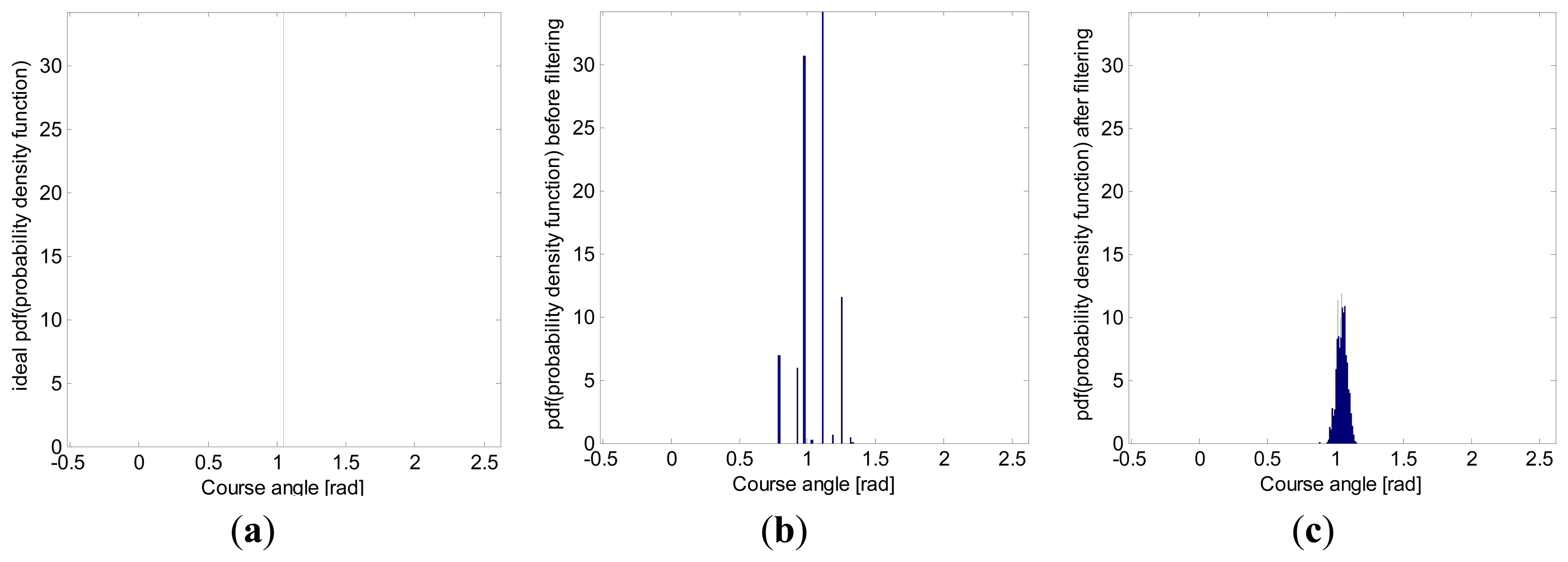
Another illustrative graph, showing the behavior of the filtering along straight lines, is the heading angle histogram. As Figure 12 shows, the proposed Kalman filter meaningfully reduced the spread from the real heading angle.
The standard deviation and the 95th-percentile range, computed from the heading angle histogram in Figure 12, are shown in Table 2, in which the standard deviation was reduced by 73.62% in the simulations with artificial data.
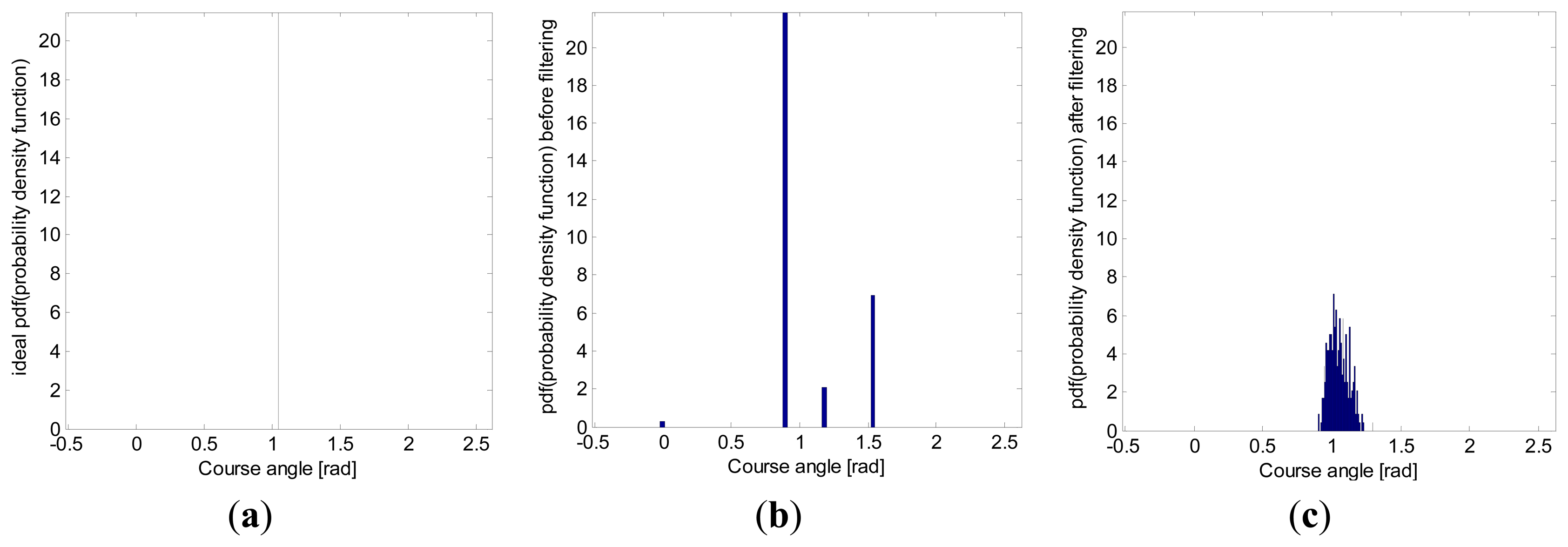
Another heading angle histogram was also computed, this time with experimental data acquired from a low-cost Navilock NL-402U GPS receiver (Figure 13). As with simulations, the filtering also avoided great changes of heading angle, thus achieving a smoother path.
The standard deviation and the 95th-percentile range, computed from the heading angle histogram in Figure 13, are shown in Table 3. As this table shows, the standard deviation was also reduced by around 75.04% in the real field tests.
4. Discussion
The main finding of the present study is that implementation of the Kalman filter can reduce the quantization errors in the positioning of tractors equipped with some low-cost GPS receivers by 43%. Moreover, it reduces by 75% the standard deviation of the heading angle.
Several studies have shown that GPS accuracy can range from 1–2 cm to 100 m [34–36] depending on the kind of GPS receiver and of the type of corrections employed. For low-cost GPS receivers using Wide Area Augmentation System (WAAS) or European Geostationary Navigation Overlay Service (EGNOS) corrections, position accuracy of 95% time can be less than 3 m [37–39]. In contrast, relative accuracy or pass-to-pass accuracy [10] is the really important variable for multiple agricultural applications. In experimental tests, Alonso-Garcia et al. [40] found that this relative accuracy can be reduced to approximately 1 m over short time periods of about 15 min, when using low-cost GPS receivers. This relative accuracy could be enough for agricultural applications with wide working widths, such as fertilizing applications. In fact, some companies, such as Agroguia® [7] and Tractordrive® [12] in Spain, sell tractor GPS guidance assistance systems equipped with low-cost GPS receivers.
In a previous study, this research team has proposed a way of improving the precision of GPS tractor positioning [41]. Moreover, the authors have acquired expertise in their work on tractor GPS guidance systems with two Spanish companies: Agroguia® [7] and Tractordrive® [12]. In their experience, the GPS receivers with the best price-precision ratios for agricultural tasks, on the market from 2008–2013, were low-cost GPS receivers equipped with Sirf IV and U-blox 4 chipsets. Nevertheless, GPS receivers equipped with these chipsets offer geodetic latitude and longitude with only 8 and 9 digits, respectively. When these coordinates are converted to Cartesian coordinates by the GPS guidance system, the positions fit in a quantization grid, the dimensions of which vary in accordance with the point on the terrestrial surface. In Valladolid, Spain, the grid is about 14 and 18 cm, on the X and the Y axes, respectively. Tractor guidance systems that employ positions within this grid suffer from oscillations in the representation of the tractor trajectory. Besides, the GPS data with heading oscillation complicate the steering of the tractor. The proposed Kalman filter is especially useful for tractor guidance assistance systems equipped with GPS receivers that have Sirf IV and U-blox 4 chipsets. It smooths the quantized sharp trajectory and provides more accurate heading information, closer to the real data, thereby facilitating the steering of the tractor.
Tractors usually move over rough surfaces, and then, although a tractor goes along a straight trajectory, the GPS receiver will acquire a sharp trajectory. This is due to the lateral vibrations experienced by the GPS receiver, which is placed over the tractor cab, two or three meters above-ground. At this position, the vertical displacement of the tractor wheels is converted into lateral vibrations. As a numerical example, a typical 10 cm vertical displacement of one rear wheel of the tractor can lead to a lateral displacement of the GPS receiver of up to 30 cm. Our implementation of the Kalman filter will be useful in these situations, because it will smooth the sharp trajectory due to vibrations and will provide more accurate heading information, close to the real data. Similar studies to remove noise from GPS data have been presented in the literature [42]. The main difference of our article and the one proposed by Han et al. [42] is the Kalman filter tuning mode; Han et al. tuned it by trial and error whereas we applied Monte Carlo techniques to eighteen trajectories to obtain the covariance matrices that produce the lowest Root Mean Square Error.
Overall, our data suggest that the proposed filter is adequate for data preprocessing of some low-cost GPS receivers, when used in GPS assisted-guidance systems for tractors. It also could be useful to smooth the GPS trajectories that are sharpened due to the tractor moving over rough terrain.
One limitation of this study is that the proposed Kalman filter reduces the quantization error in GPS receivers that provide geodetic latitude and longitude with eight and nine digits, but, in GPS receivers that provide more digits, the reduction in the quantization error does not exist or is negligible. Microelectronics technology progresses quickly. Hopefully, in a few years all GPS receivers in the market, high end and low cost, will be equipped with chipsets that provide positioning data with enough digits, so that the quantization effects are negligible. Nevertheless, today, our proposed Kalman filter is at present useful for processing the data of some low-cost GPS receivers. Moreover, in the future the filter will be useful for the preprocessing of GPS trajectories on tractors moving over rough surfaces. A second drawback of our proposed Kalman filter is that, besides smoothing errors, as a side effect real deviations are also smoothed. This effect could be negative in some systems, as for example the used in GPS assisted guidance of tractors.
Further studies could be conducted. A more detailed quantitative analysis about inherent delays of the proposed system, both along both straight and curve paths, could be addressed. Besides, because most low-cost GPS receivers provide positioning information at 1 Hz rate, simple modifications to the Kalman filter proposed in this paper could be employed to increase the positioning rate. Modifications could also be used to fuse the data from low-cost GPS receivers with local positioning systems as gyroscopes and compasses employing, for example, Arduino® or Raspberry Pi® boards. Since nowadays most modern smartphones also include gyroscopes and compasses, it will be possible to deploy this system using a smartphone that fuses the data from its own sensors.
5. Conclusions
In summary, certain low-cost GPS receivers, such as those equipped with Sirf IV and U-blox 4 chipsets, offer positioning information by using NMEA with eight digits for geodetic latitude and nine for longitude. When these geodetic coordinates are converted into Cartesian coordinates, the positions fit in a quantization grid. The dimensions of the quantization grid vary for each point on the terrestrial surface and usually range some decimeters in size. The Kalman filter implementation in this study, applied to data from these low-cost GPS receivers, has reduced the quantization errors by 43% and the standard deviation of the heading by 75%, without introducing positioning delays. On the basis of our data, we consider that use of the filter improves the precision of low-cost GPS receivers in some agricultural tasks, such as GPS assisted-guidance of tractors. It also could be useful to smooth tractor GPS trajectories that are sharpened when the tractor moves over rough terrain.
Conflicts of Interest
The authors declare no conflict of interest.
References
- Slaughter, D.C.; Giles, D.K.; Downey, D. Autonomous robotic weed control systems: A review. Comput. Electron. Agric. 2008, 61, 63–78. [Google Scholar]
- Zhang, N.; Wang, M.; Wang, N. Precision agriculture—a worldwide overview. Comput. Electron. Agric. 2002, 36, 113–132. [Google Scholar]
- Auernhammer, H. Precision farming—the environmental challenge. Comput. Electron. Agric. 2001, 30, 31–43. [Google Scholar]
- Keicher, R.; Seufert, H. Automatic guidance for agricultural vehicles in Europe. Comput. Electron. Agric. 2000, 25, 169–194. [Google Scholar]
- Li, M.; Imou, K.; Wakabayashi, K.; Yokoyama, S. Review of research on agricultural vehicle autonomous guidance. Int. J. Agric. Biol. Eng. 2009, 2, 1–16. [Google Scholar]
- Holden, N.M.; Comparetti, A.; Ward, S.M.; McGovern, E.A. Accuracy assessment and position correction for low-cost non-differential GPS as applied on an industrial peat bog. Comput. Electron. Agric. 1999, 24, 119–130. [Google Scholar]
- Agroguia. Available online: http://www.agroguia.es (accessed on 16 August 2012).
- Tractordrive. Available online: http://www.tractordrive.es (accessed on 16 August 2012).
- August, P.; Michaud, J.; Lavash, C.; Smith, C. GPS for environmental applications: Accuracy and precision of locational data. Photogramm. Eng. Remote Sens. 1994, 60, 41–45. [Google Scholar]
- Tractors and Machinery for Agriculture and Forestry—Test Procedures for Positioning and Guidance Systems in Agriculture—Part 1: Dynamic Testing of Satellite-Based Positioning Devices. Available online: https://www.iso.org/obp/ui/#iso:std:iso:12188:-1:ed-1:v1:en (accessed on 7 November 2013).
- Tractors and Machinery for Agriculture and Forestry—Test Procedures for Positioning and Guidance Systems in Agriculture—Part 2: Testing of Satellite-Based Auto-Guidance Systems during Straight and Level Travel. Available online: https://www.iso.org/obp/ui/#iso:std:iso:12188:-2:ed-1:v1:en (accessed on 7 November 2013).
- Cambridge Silicon Radio Plc. Available online: http://www.csr.com (accessed on 16 August 2012).
- U-Blox. Available online: http://www.u-blox.com (accessed on 16 August 2012).
- MediaTek Inc. Available online: http://www.mediatek.com/en (accessed on 16 August 2012).
- Smith, S.O. The Universal Grids: Universal Transverse Mercator (UTM) and Universal Polar Sterographic (UPS); DMA TM 8358.2; Defense Mapping Agency: Washington, DC, USA, 1989. [Google Scholar]
- Snyder, J.P. Map Projections—A Working Manual, 1st ed.; United States Government Printing: Washington, DC, USA, 1987; p. p. 383. [Google Scholar]
- Pearson, F. Map Projections: Theory and Applications, 2nd ed.; CRC Press: Boca Raton, FL, USA, 1990; p. p. 384. [Google Scholar]
- Grewal, M.S.; Weill, L.R.; Andrews, A.P. Appendix C: Coordinate Transformations. In Global Positioning Systems, Inertial Navigation, and Integration, 2nd ed.; John Wiley & Sons: Hoboken, NJ, USA, 2007; p. p. 552. [Google Scholar]
- Latombe, J.-C. Robot Motion Planning, 1st ed.; Kluwer Academic Publishers: Norwell, MA, USA, 1991; p. p. 672. [Google Scholar]
- Kalman, R.E. A new approach to linear filtering and prediction problems. Trans. ASME 1960, 82, 35–45. [Google Scholar]
- Brown, R.G.; Hwang, P.Y.C. The Discrete Kalman Filter, State-Space Modeling and Simulation. In Introduction to Random Signals and Applied Kalman Filtering, 3th ed.; John Wiley and Sons: Toronto, ON, Canada, 1997; pp. 190–241. [Google Scholar]
- Zarchan, P.; Musoff, H. Fundamentals of Kalman Filtering: A Practical Approach, 2nd ed.; AIAA: Alexandria, VA, USA, 2005; p. p. 664. [Google Scholar]
- Papoulis, A. Probability, Random Variables, and Stochastic Processes, 3rd ed.; McGraw-Hill: New York, NY, USA, 1991; p. p. 666. [Google Scholar]
- Åkesson, B.M.; Jørgensen, J.B.; Poulsen, N.K.; Jørgensen, S.B. A generalized autocovariance least-squares method for Kalman filter tuning. J. Process Control 2008, 18, 769–779. [Google Scholar]
- Saha, M.; Goswami, B.; Ghosh, R. Two Novel Costs for Determining the Tuning Parameters of the Kalman Filter. Proceedings of Advances in Control and Optimization of Dynamic Systems (ACODS-2012), Bangalore, India; 2012; pp. 1–8. [Google Scholar]
- Bodizs, L.; Srinivasan, B.; Bonvin, D. Preferential Estimation via Tuning of the Kalman Filter. Proceedings of 7th International Symposium on Dynamics and Control of Process Systems (DYCOPS7), Cambridge, MA, USA; 2004. [Google Scholar]
- Loebis, D.; Sutton, R.; Chudley, J.; Naeem, W. Adaptive tuning of a Kalman filter via fuzzy logic for an intelligent AUV navigation system. Control Eng. Prac. 2004, 12, 1531–1539. [Google Scholar]
- Korniyenko, O.V.; Sharawi, M.S.; Aloi, D.N. Neural Network Based Approach for Tuning Kalman Filter. Proceedings of IEEE International Conference on Electro Information Technology, Lincoln, NE, USA; 2005; pp. 1–5. [Google Scholar]
- Goodall, C.; El-Sheimy, N. Intelligent Tuning of a Kalman Filter Using Low-Cost MEMS Inertial Sensors. Proceedings of 5th International Symposium on Mobile Mapping Technology (MMT'07), Padua, Italy; 2007; pp. 1–8. [Google Scholar]
- Ran, C.; Deng, Z. Self-tuning weighted measurement fusion Kalman filter and its convergence. J. Control Theory Appl. 2010, 8, 435–440. [Google Scholar]
- Mosavi, M.R.; Sadeghian, M.; Saeidi, S. Increasing DGPS navigation accuracy using Kalman filter tuned by genetic algorithm. Int. J. Comput. Sci. Issues 2011, 8, 246–252. [Google Scholar]
- Stroud, P.D. Kalman-extended genetic algorithm for search in nonstationary environments with noisy fitness evaluations. IEEE Trans. Evol. Comput. 2001, 5, 66–77. [Google Scholar]
- Liu, J.S. Monte Carlo Strategies in Scientific Computing, 1st ed.; Springer: Cambridge, MA, USA, 2009; p. p. 344. [Google Scholar]
- Czajewski, J. The accuracy of the global positioning systems. IEEE Instrum. Meas. Mag. 2004, 40, 56–60. [Google Scholar]
- Gan-Mor, S.; Clark, R.L.; Upchurch, B.L. Implement lateral position accuracy under RTK-GPS tractor guidance. Comput. Electron. Agric. 2007, 59, 31–38. [Google Scholar]
- Valbuena, R.; Mauro, F.; Rodríguez-Solano, R.; Manzanera, J.A. Accuracy and precision of GPS receivers under forest canopies in a mountain environment. Span. J. Agric. Res. 2010, 8, 1047–1057. [Google Scholar]
- Peters, R.T.; Evett, S.R. Using low cost GPS receivers for determining field position of mechanized irrigation systems. Appl. Eng. Agric. 2005, 21, 841–845. [Google Scholar]
- Witte, T.H.; Wilson, A.M. Accuracy of WAAS-enabled GPS for the determination of position and speed over ground. J. Biomech. 2005, 38, 1717–1722. [Google Scholar]
- Arnold, L.L.; Zandbergen, P.A. Positional accuracy of the wide area augmentation system in consumer-grade GPS units. Comput. Geosci. 2011, 37, 883–892. [Google Scholar]
- Alonso-Garcia, S.; Gomez-Gil, J.; Arribas, J.I. Evaluation of the use of low-cost GPS receivers in the autonomous guidance of agricultural tractors. Span. J. Agric. Res. 2011, 9, 377–388. [Google Scholar]
- Gomez-Gil, J.; Alonso-Garcia, S.; Gomez-Gil, F.J.; Stombaugh, T. A simple method to improve autonomous gps positioning for tractors. Sensors 2011, 11, 5630–5644. [Google Scholar]
- Han, S.; Zhang, Q.; Noh, H. Kalman filtering of DGPS positions for a parallel tracking application. Trans. ASAE 2002, 45, 553–559. [Google Scholar]


| Before Filtering | After Filtering | |
|---|---|---|
| Distances Root-Mean Square Error (RMSE) (cm) | 6.56 | 3.74 |
| Distances 95th-percentile (cm) | 8.48 | 4.31 |
| Before Filtering | After Filtering | |
|---|---|---|
| Standard deviation (°) | 6.9362 | 1.8301 |
| 95th-percentile range (centered on real heading angle) (°) | 29.0661 | 7.2651 |
| Before Filtering | After Filtering | |
|---|---|---|
| Standard deviation (°) | 16.5594 | 4.1326 |
| 95th-percentile range (centered on reference heading angle) (°) | 55.1185 | 14.7193 |
© 2013 by the authors; licensee MDPI, Basel, Switzerland. This article is an open access article distributed under the terms and conditions of the Creative Commons Attribution license (http://creativecommons.org/licenses/by/3.0/).
Share and Cite
Gomez-Gil, J.; Ruiz-Gonzalez, R.; Alonso-Garcia, S.; Gomez-Gil, F.J. A Kalman Filter Implementation for Precision Improvement in Low-Cost GPS Positioning of Tractors. Sensors 2013, 13, 15307-15323. https://doi.org/10.3390/s131115307
Gomez-Gil J, Ruiz-Gonzalez R, Alonso-Garcia S, Gomez-Gil FJ. A Kalman Filter Implementation for Precision Improvement in Low-Cost GPS Positioning of Tractors. Sensors. 2013; 13(11):15307-15323. https://doi.org/10.3390/s131115307
Chicago/Turabian StyleGomez-Gil, Jaime, Ruben Ruiz-Gonzalez, Sergio Alonso-Garcia, and Francisco Javier Gomez-Gil. 2013. "A Kalman Filter Implementation for Precision Improvement in Low-Cost GPS Positioning of Tractors" Sensors 13, no. 11: 15307-15323. https://doi.org/10.3390/s131115307