An atomic force microscope (AFM) is composed of a micro-machined cantilever with nulling control devices, vertical and horizontal scanners (usually, monolithic tube piezoelectric scanners), an optical microscope for viewing the cantilever and samples, and coarse positioning devices for the cantilever and the sample [1]. The optical microscopes are configured into two types. One type is on-axis, wherein the optical center axis of the optical microscope coincides with the cantilever’s axis. The other type is off-axis, wherein the optical axis of the optical microscope doesn’t coincide with the cantilever’s axis. Because the viewing angle of the on-axis optical microscope is limited, the AFM head, including the vertical scanner, must not interfere with the viewing angle for clear imaging of the cantilever and sample. In addition, previous studies have mainly considered horizontal xy-scanners [2–5] or the coupled xyz-scanner [6]. Recently, the compact two-axis scanner with scan range of 10 μm × 10 μm was developed for high speed scanning [7].

We have developed a compact vertical scanner that has no interference with the viewing angle of the optical microscope. The scanner is composed of a linear flexure guide, a piezoelectric actuator, and a feedback sensor. The theoretical stiffness of the flexure guide is analyzed, and its resonance is calculated and verified using finite element analysis. The optimal design technique is used to maximize the feedback speed, and the result is verified using finite element analysis. The travel range, feedback noise, nulling resolution, and resonances were evaluated experimentally and compared to the theoretical findings. Finally, we present an AFM image from the developed vertical scanner.

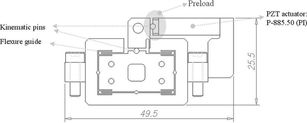
A z-scanner serves as a vertical fine scanner for the nulling control of an optical lever. A diagram of the z-scanner is shown in Figure 1. The flexure guide is used as a guide mechanism. A PZT actuator is attached to the flexure guide via a kinematic pin. Because the PZT actuator is fragile with respect to tension and moment loading, it cannot be glued into the guide. As a solution, an appropriate preload is applied to the flexure guide during assembly to prevent detachment between the actuator and the guide. Accordingly, the preloading effect should be considered in the optimal design. The critical design point of the scanner is as follows. Because the working distance and the viewing angle of the objective lens are fixed, the height and the overall dimension of the z-scanner should be minimized for viewing the cantilever. In this study, so as not to interfere with the viewing angle of the objective lens, the PZT actuator’s horizontal deformations are transferred to the vertical flexure guide via the circular hinge and the two kinematic pins. Moreover, the resonant frequency should be high enough for fast nulling control.

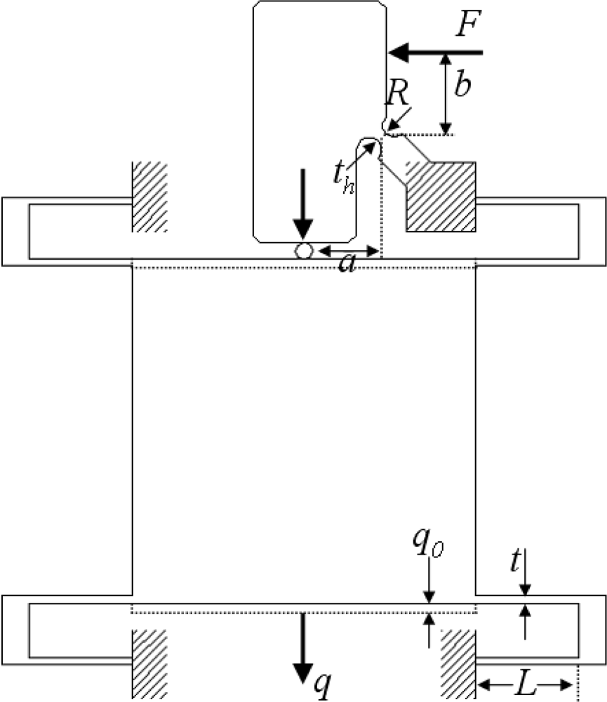
For the model, the z-scanner is simplified as shown in Figure 2. F is a force exerted by the PZT actuator; R, t_h, and w_h are the radius, thickness, and depth (width) of the rotational hinge, respectively; L, t, and w are the length, thickness, and depth (width) of the flexure guide; and q and q₀ are displacement and initial preload of the moving body, respectively.

The static stiffness of the flexure guide is given by [8]: (1) k f = 24 E I L 3where E is Young’s modulus and I (= wt³/12) is the second moment of inertia of the flexure guide. The stiffness (N/m) of the rotational hinge for changing of the force exerted by the PZT actuator is calculated as follows: (2) k h = 2 E w h t 2.5 9 π R 0.5 a b

Therefore, the total stiffness of the z-scanner is given by: (3) k t = k f + k h = 24 E I L 3 + 2 E w h t 2.5 9 π R 0.5 a b

Using Equation (3) and considering the PZT specifications, the displacement of the flexure guide due to the PZT force is given by: (4) q = F max d max F max + d max k t − d max k t q 0 F max + d max k twhere F_max and d_max are the maximum force and the maximum displacement of the PZT actuator at the full voltage input. As described in Equation (4), the initial preload q₀ decreases the total displacement.

Using Equation (3), the natural frequency of the flexure guide is calculated as follows: (5) f n = 1 2 π k f / m fwhere m_f is the moving mass of the flexure guide.

The optimal design is determined with the objective of maximizing the resonant frequency. Thus, the cost function is given by: (6) J = min ( 1 f s 2 )

The cost function has two constraints: the maximum displacement should be larger than 17 μm, and the maximum stress should be lower than 20% of the ultimate strength of the material. The maximum stress was selected considering the fatigue fracture based on the following equation: (7) S n = ɛ C L C G C S S nnwhere S_n is the actual endurance limit after 10⁸ cycles, ɛ is the uncertainty (0.92) in the endurance limit, C_L is the load factor (1 for bending), C_G is the gradient factor (0.9), C_S is the surface factor (0.9 for a commercially polished surface), and S_nn is the endurance limit of the ideal material (0.35 × S_u (ultimate strength)). Therefore, S_n = 0.26 × S_u. The maximum stress was selected to be lower than 20% of the ultimate strength of the material, thereby allowing for some margin. The constraint equations are summarized as follows: (8) q max > 17   μ m σ max < 0.2 ( S u )

The optimal parameters were selected as shown in Table 1.

Using the sequential quadratic programming (SQP) method of MATLAB^® Optimization Toolbox™ (The MathWorks), the convergence plot after completion of the optimization process was determined as shown in Figure 3.

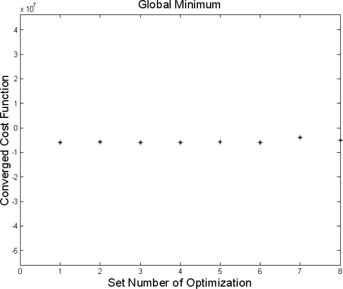
To ensure a global minimum value, eight optimization processes with random initial values were performed as shown in Figure 4. The optimized values are summarized as shown in Table 2.

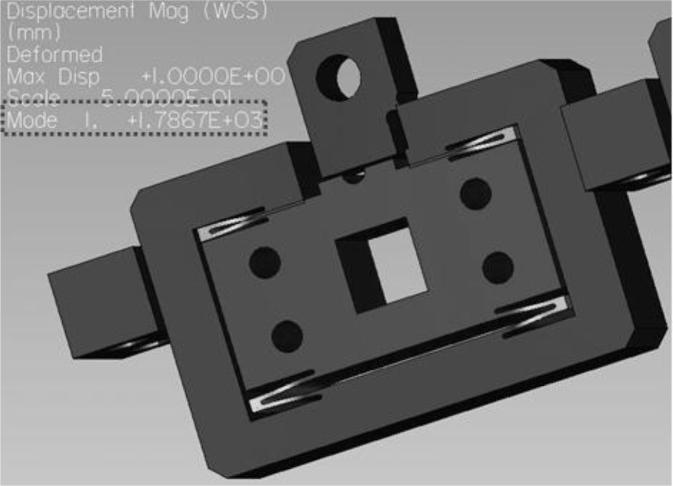
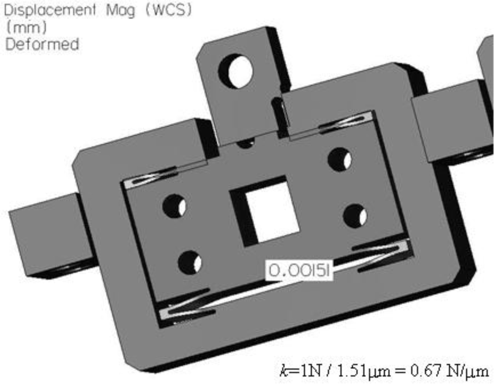
To validate the optimal design, finite element analyses using the commercial program Pro/ENGINEER Mechanica™ were performed, and the results are shown in Figure 5 and Figure 6. The stiffness simulation result is shown in Figure 5 and the first resonant frequency is shown in Figure 6. The comparison between the optimal design and the FEA results are summarized in Table 3. The difference is within 10%, which is acceptable. If the total moving mass, including the optical lever, is considered in the calculation of the resonant frequency, the final resonant frequency is 2.1 kHz.

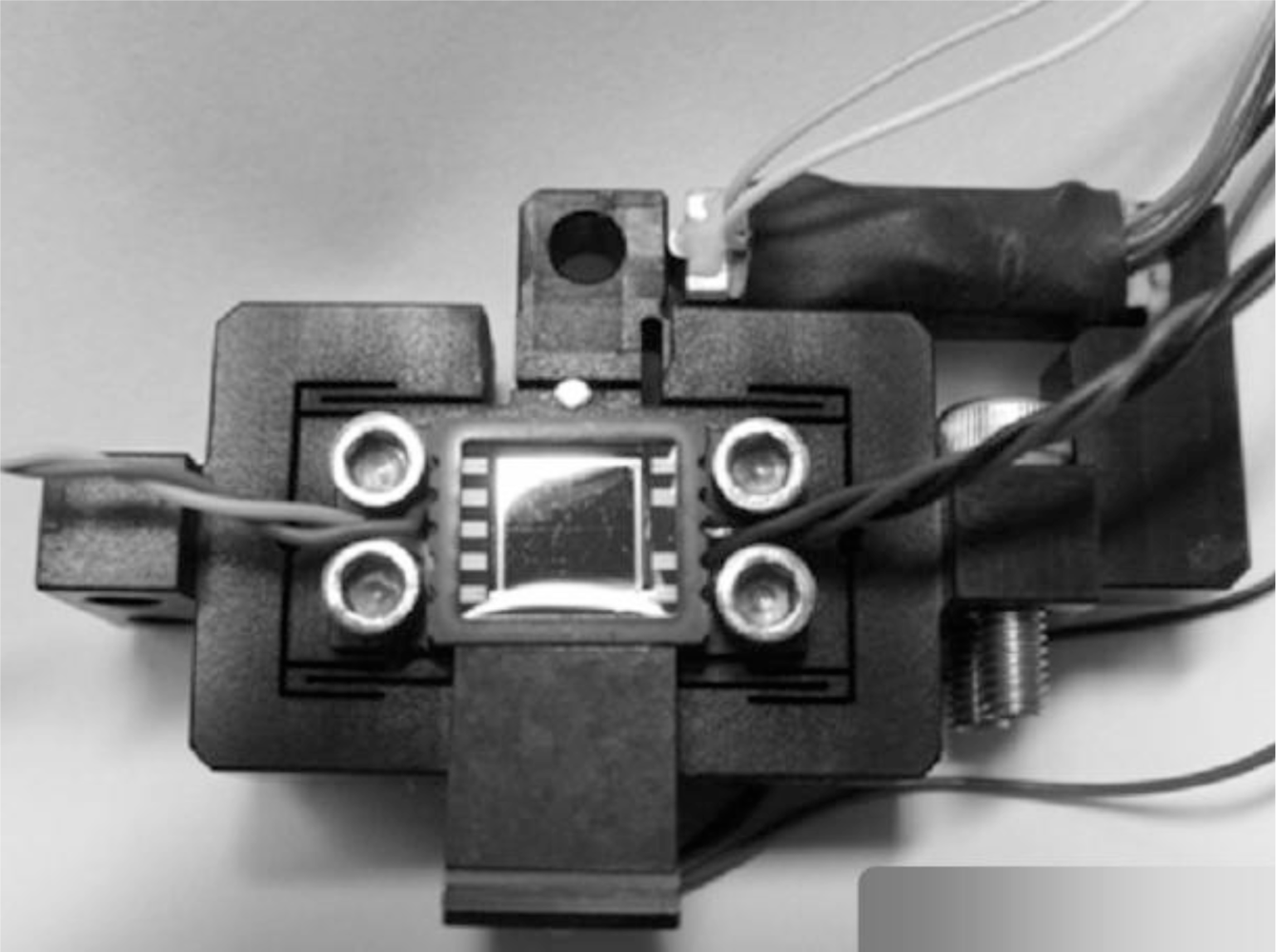
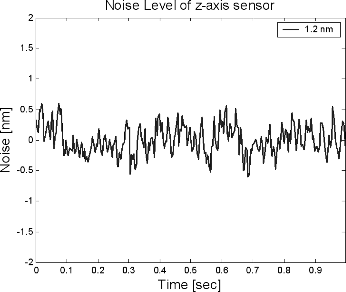
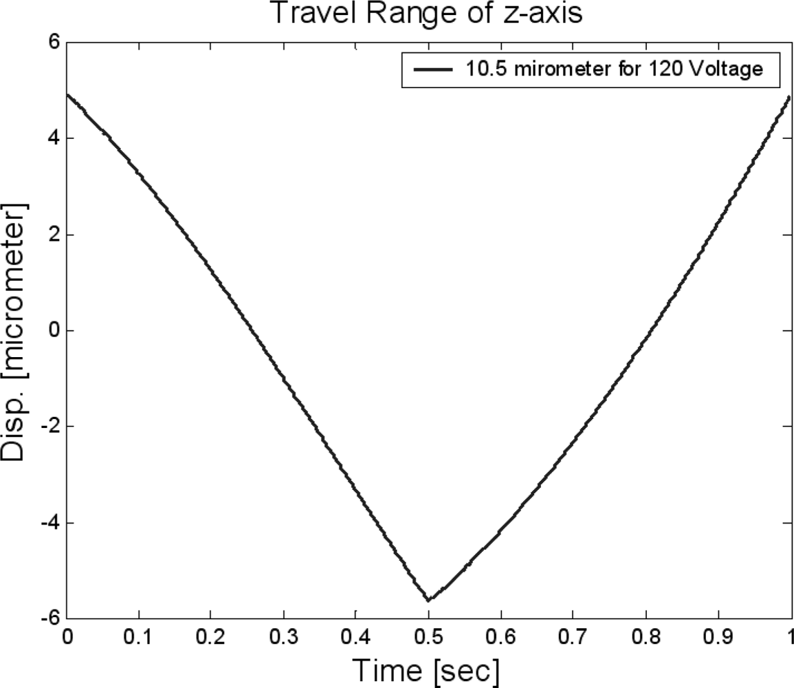
The assembled z-scanner is shown in Figure 7. The travel range of the z-scanner is shown in Figure 8. Here, the range is about 10.5 μm. The input voltage is about 120 V for protection of the PZT actuator. If an input voltage of 140 V (which is the maximum input voltage for the PZT actuator) is given, the travel range would increase to 13 μm which is close to the final goal of the design. The resolution was measured as shown in Figure 9. The noise is about 1.2 nm peak-to-peak. Also, the resonance was measured as shown in Figure 10. The first resonance is about 2 kHz, which is close to the optimal design result.

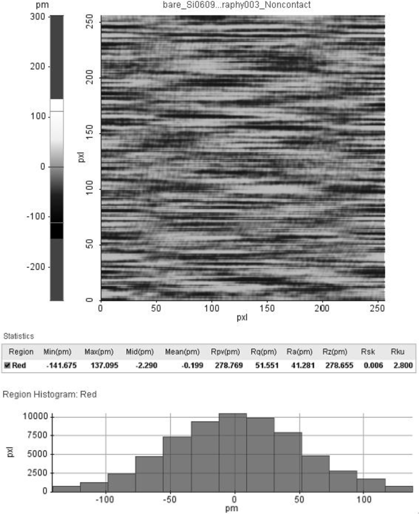
As a first measurement, the vertical nulling resolution of the total system is an important factor that determines the quality of the AFM image. The vertical nulling resolution characterizes the stability of maintaining the gap between the tip and sample. After approaching the tip close to the sample surface, we measured the gap between the tip and sample using the optical lever of the AFM head at the null state of the cantilever with no xy scanning. In this situation, a vertical AFM signal is generated by external noise (floor vibration, etc.) and internal electronic noise. This vertical AFM signal corresponds to the vertical resolution of the AFM because there is no meaningful atomic force or scanning. Figure 11 shows a histogram of the gap between the tip and sample. The vertical resolution was measured as 0.05 nm root-mean-square (RMS) from Figure 11.

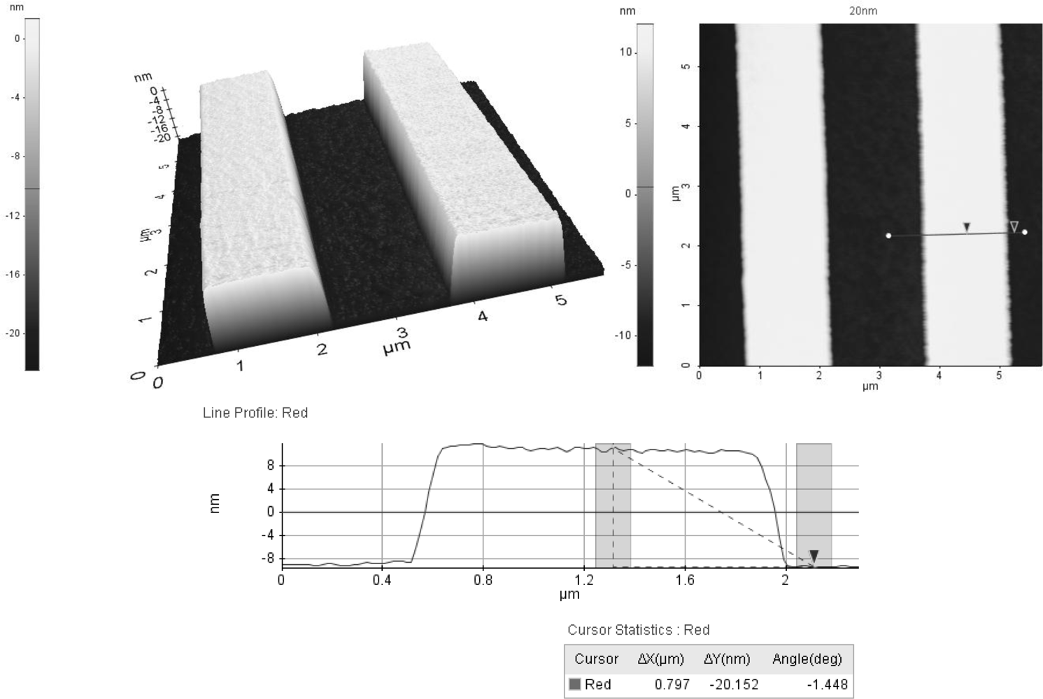
The step height (20 nm) standard sample was measured using our homemade AFM with the proposed vertical scanner as shown in Figure 12. The step height sample is clearly shown in the figure, and the vertical scanner was shown to be useful and applicable to the AFM.

A compact AFM vertical scanner that has no interference with the viewing angle of the optical microscope was developed. The theoretical stiffness of the flexure guide was analyzed, and the resonance was calculated and verified via finite element analysis. A design optimization process to maximize the feedback speed was performed and verified via finite element analysis. The travel range, feedback noise, nulling resolution, and resonances were experimentally evaluated and compared to the theoretical findings. The travel range was measured as 10.5 μm for a 120 V input. The feedback noise was about 1.2 nm peak-to-peak. The first resonance is about 2 kHz, which is close to the optimal design results. Finally, a non-contact AFM image of the 20 nm height standard sample was generated. As a final comment, the travel range of the scanner is about 10 μm that seems to be large for the specialized wafer industries. Because the usual measuring height is less than 1 μm in the wafer industries, so the small actuator could be used for the above specialized application field. If the nano-scanner is made from the vacuum compatible materials, the nano-scanner could be used in the scanning electron microscope.

References

- Kwon, J; Hong, J; Kim, YS; Lee, DY; Lee, K; Lee, SM; Park, SI. Atomic force microscope with improved scan accuracy, scan speed and optical vision. Rev Sci Instr 2003, 74, 4378–4383. [Google Scholar]
- Choi, KB; Lee, JJ; Hata, S. A piezo-driven compliant stage with double mechanical amplification mechanisms arranged in parallel. Sens Actuat A-Phys 2010, 161, 173–181. [Google Scholar]
- Kwon, S; Milanovic, V; Lee, LP. Large-displacement vertical microlens scanner with low driving voltage. IEEE Photonic Technol Lett 2002, 14, 1572–1574. [Google Scholar]
- Choi, KB; Kim, DH. Monolithic parallel linear compliant mechanism for two axes ultraprecision linear motion. Rev Sci Instr 2006, 77, 1–6. [Google Scholar]
- Kang, D; Kim, K; Kim, D; Shim, J; Gweon, DG; Jeong, J. Optimal design of high precision XY-scanner with nanometer-level resolution and millimeter-level working range. Mechatronics 2009, 19, 562–570. [Google Scholar]
- Schitter, G; Astrom, KJ; DeMartini, BE; Thurner, PJ; Turner, KL; Hansma, PK. Design and modeling of a high-speed AFM-scanner. IEEE Trans Control Syst Techn 2007, 15, 906–915. [Google Scholar]
- Leang, KK; Fleming, AJ. High-speed serial-kinematic AFM scanner: Design and drive considerations. Asian J. Control 2009, 11, 144–153. [Google Scholar]
- Smith, ST. Flexure: Elements of Elastic Mechanics; Taylor and Francis: London, UK, 2003; p. 209. [Google Scholar]