Article

Identification and Density Estimation of American Martens (Martes americana) Using a Novel Camera-Trap Method

1
Department of Natural Resources and the Environment, University of New Hampshire, Durham, NH 03824, USA
2
DOI Northeast Climate Science Center, University of Massachusetts, Amherst, MA 01003, USA
*
Author to whom correspondence should be addressed.
Diversity 2016, 8(1), 3; https://doi.org/10.3390/d8010003
Submission received: 1 November 2015 / Revised: 31 December 2015 / Accepted: 7 January 2016 / Published: 12 January 2016
(This article belongs to the Special Issue Camera Traps in Animal Ecology)

Abstract

:
Camera-traps are increasingly used to estimate wildlife abundance, yet few studies exist for small-sized carnivores or comparing efficacy against traditional methods. We developed a camera-trap to identify the unique ventral patches of American martens (Martes americana). Our method was designed to: (1) determine the optimal trap configuration to photograph ventral patches; (2) evaluate the use of temporally clustered photographs to determine independence and improve identification; and (3) determine factors that influence identification probability. We tested our method by comparing camera- and live-trap density estimates using spatial capture–recapture (SCR) models. The ventral patches of radio-collared martens were most visible when traps were placed 15–20 cm above a feeding platform. Radio-collared martens (n = 14) visited camera-traps for long periods (median = 7 min) with long intervals between visits (median = 419 min), and visits by different martens at the same trap <15 min apart was infrequent (n = 3) during both years. Similarly, there was complete agreement among observers that clustered photos of un-collared martens were always of the same individual. Pairwise agreement was high between observers; eight un-collared martens were identifiable by consensus on 90% (54 of 60) of recorded visits. Factors influencing identification probability were directly related to the time martens spent feeding at traps (β = 0.143, P = 0.01) and inversely proportional to the time that elapsed since traps were baited (β = −0.344, P = 0.006). Density estimates were higher and more precise for camera-trapping (0.60, 0.35–1.01 martens/km2) than live-trapping (0.45, 0.16–1.22 martens/km2), providing evidence that SCR density estimates may be biased when capture heterogeneity is present, yet cannot be accounted for due to small sample size. Our camera-trap method provides a minimally invasive and accurate tool for monitoring marten populations.

1. Introduction

Estimating abundance is critical for effective management and conservation [1]. Many studies rely on live-trapping and radio telemetry (e.g., [2,3]). However, both methods are labor intensive, expensive, and impractical in wilderness areas with harsh climate [4]. Further, capture and handling is invasive, can elicit a behavioral response (e.g., trap shyness) that may bias population estimates [5,6], and potentially dangerous to the animal. Remotely-triggered cameras are increasingly used to identify individuals for species with unique pelage patterns [7,8], morphological characteristics [9,10], and artificial markings [11,12]. Similar to non-invasive genetic sampling [13,14], this approach can increase sample size and may reduce effort and cost [15]. However, failure to consistently identify individuals is common for camera-trap studies and can result in sampling bias if not adequately addressed [15].
American martens (Martes americana) are a prime candidate for camera-trap abundance estimation. They generally occupy remote wilderness areas throughout the northern United States and Canada [16], making it difficult to monitor populations [17]. Moreover, martens are sexually dimorphic [18,19], with unique ventral patterns that can potentially be used for individual identification [8,20], and respond positively to baited camera-traps [20] making them ideal candidates for photo identification. Importantly, density estimates are critical to provide input to conservation of this species which is sensitive to habitat loss and fragmentation [21,22,23] and predicted to decline along southern range boundaries due to climate change [24,25].
The use of camera-trapping is increasingly common [4], yet methods for analyzing its reliability are still evolving (e.g., [26,27]). Numerous sources of variability can influence photo identification of individuals, including prominence of unique markings within a population [15,28], camera angle and lighting [29], and camera brands [30]. Trap configuration can also have a significant effect [9]. Magoun et al. [8] used a baited camera-trap that required a wolverine (Gulo gulo) to reveal its ventral marks for a prolonged period while feeding. Although this design may work for martens [8], they are considerably smaller than wolverines, requiring cameras to be closer which can complicate identification [26].
The temporal distribution of photographic captures can have an impact on individual identification as well. Studies often require >1 picture to identify individuals with varying criteria for independent visits [29,31,32]. For example, Mendoza et al. [31] utilized temporally clustered bobcat (Lynx rufus) photographs at unbaited camera stations to determine independent visits and increase consensus among observers. However, if temporal activity is not evaluated or arbitrarily assigned, visits by multiple individuals within a photographic cluster may go unnoticed and violate assumptions of capture–mark–recapture analyses [15,33]. Although some misidentification errors can be explicitly modeled [34] further development is required [35]; therefore, it is prudent to screen data prior to the modeling process [31]. To our knowledge, no studies have used artificially marked individuals to evaluate temporal activity at camera-traps and assess the use of photographic clusters to improve individual identification and define independent observations.
Inconsistency among observers can also pose a problem [29,36]. To reduce observer bias, camera-trap studies have utilized ≥2 independent observers to assign the identity of individuals and construct capture histories [29,36,37]. Although this approach may reduce the proportion of individuals identified and result in a lower sample size [29], culling erroneous identity assignments can increase the accuracy of density estimates [15]. Further, while automated computer software provides accurate assignments and saves time, it does not always perform well with the poor quality pictures that occur in camera-trap studies [38,39]. Variation caused by shadows, camera angles, scale, time of day, and different camera brands make automated computer processing difficult [40].
Recent spatial capture–recapture (SCR) models incorporate the movement of individuals between trap locations, resolving the influence of space on both the ecological and observational processes that generate capture–recapture data [41,42]. Compared with SCR models, buffer methods (e.g., 0.5× mean maximum distance moved; [43]) may provide biased estimates of density [2,44,45], except when home ranges are elongated or irregular [46]. The SCR approach provides flexible model selection for researchers and can be useful for studies with small sample size and imbalanced designs [41,42,47]. Because SCR models are used increasingly for minimally invasive surveys, it is important to evaluate performance with empirical data [15] and compare with traditional methods (e.g., live-trapping) to validate the method [26,48].
We documented camera-trap visits by radio-collared martens with unique artificial markings and un-collared martens over two winters in a remote forest in northern New Hampshire. Our objectives were to: (1) identify the optimal camera-trap configuration to effectively photograph marten ventral patches of both sexes; (2) evaluate the use of temporally clustered photographs of radio-collared martens to improve identification of individuals and determine independence; (3) utilize observers to record the total number of un-collared individuals, identify the proportion of unique captures that were identifiable, and develop a capture history; (4) determine factors that influenced identification probability of photo captured martens; and (5) compare camera- and live-trapping datasets using a SCR modeling framework to evaluate the hypothesis that camera-trapping would provide more accurate and precise density estimates due to increased recaptures and longer effort.

2. Experimental Section
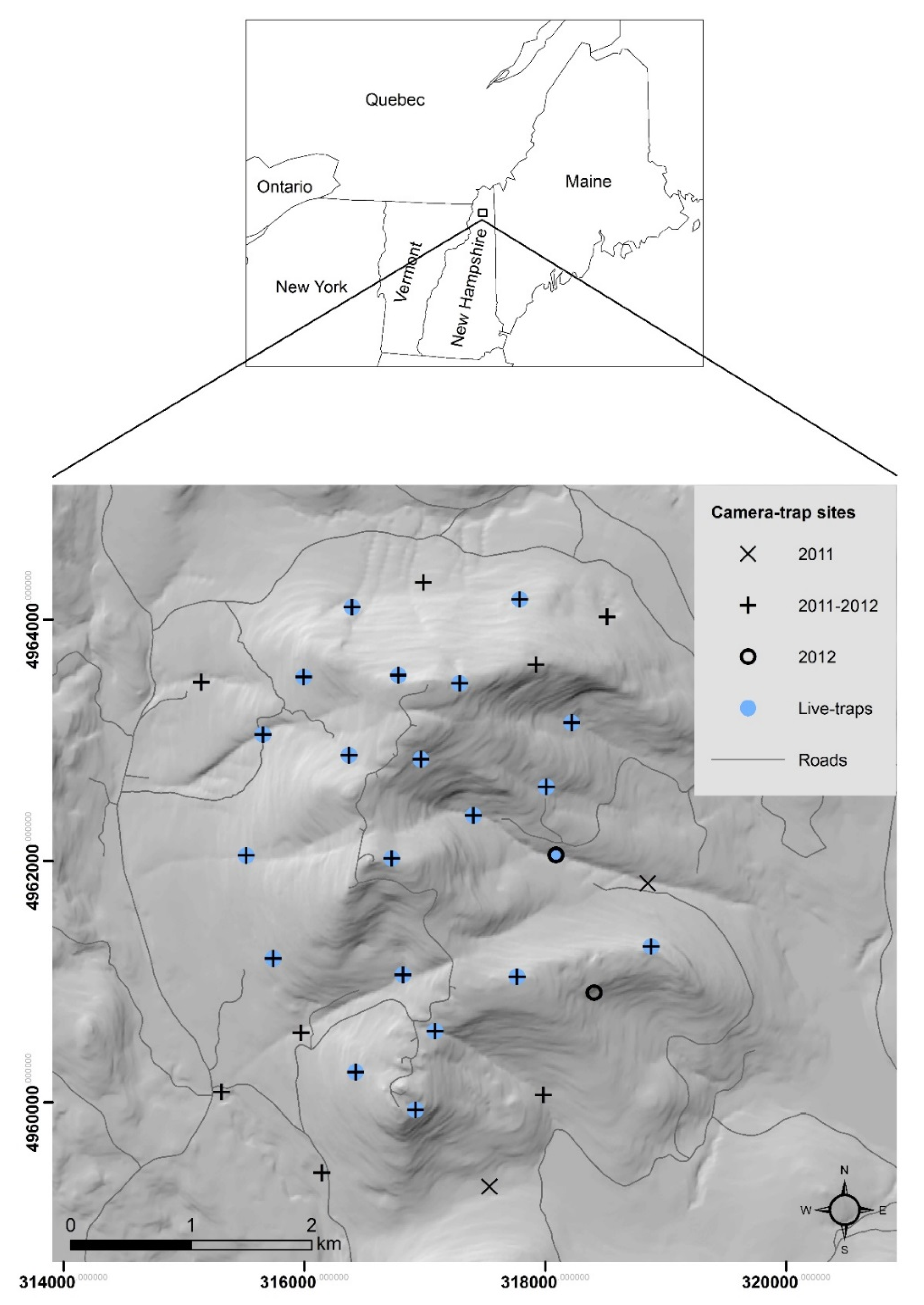
2.1. Study Area

We tested our camera-trap method on an American marten population located in the New England-Acadian Forest [49] of northern New Hampshire, USA (Figure 1). The regional climate is characterized by warm and wet summers and cold winters with deep snow. Annual precipitation ranges between 91–178 cm and snowfall varies 244–406 cm, with deeper snow at higher elevations and in the northern part of the state [50]. Temperature ranges considerably with January the coldest month ( x - = −11 °C (−15 to −2 °C)) and July the warmest ( x - = 18 °C (11 to 27 °C); [50]). The study area was mountainous for the region (624–1045 m) and primarily forested with a mixture of mature and commercially harvested lowland forest and predominantly mature forest at high elevation [51].
Figure 1. Study area used to develop the camera-trap method to identify radio-collared and un-collared American martens (Martes americana) and estimate density in northern New Hampshire, USA.
Diversity 08 00003 g001

2.2. Live-Trapping

We conducted live-trapping seasonally from 2010–2012 to maintain a sample size of 6–10 radio-collared martens to evaluate the effectiveness of the camera-trap design and for density estimation. Live-traps (Model #102; Tomahawk Live Trap, Hazelhurst, WI, USA) were established in known marten habitat [trees >6 m tall; 21], weatherproofed, baited with sardines, and a commercial skunk lure was used to attract marten into traps. Live-traps were checked at least once daily and captured marten were restrained using a handling cone and injected intramuscularly with a 5:1 mixture of ketamine hydrochloride:xylazine hydrochloride [52]. Sex was determined and age (juvenile or adult) was estimated by palpation of the cranial ridge (males only) and examining teeth for wear and coloration after animals were fully immobilized (~2 min). A numbered ear tag (Monel no. 1; National Band and Tag Co., Newport, KY, USA) was placed in each ear and artificial markings were adhered on radio-collars to identify individuals during camera-trapping. All immobilized and recaptured martens were given an electrolyte drink and raspberry jam, and released immediately after processing or identification. Live-trapping and handling procedures were approved by the Institutional Animal Care and Use Committee, University of New Hampshire (#100807).

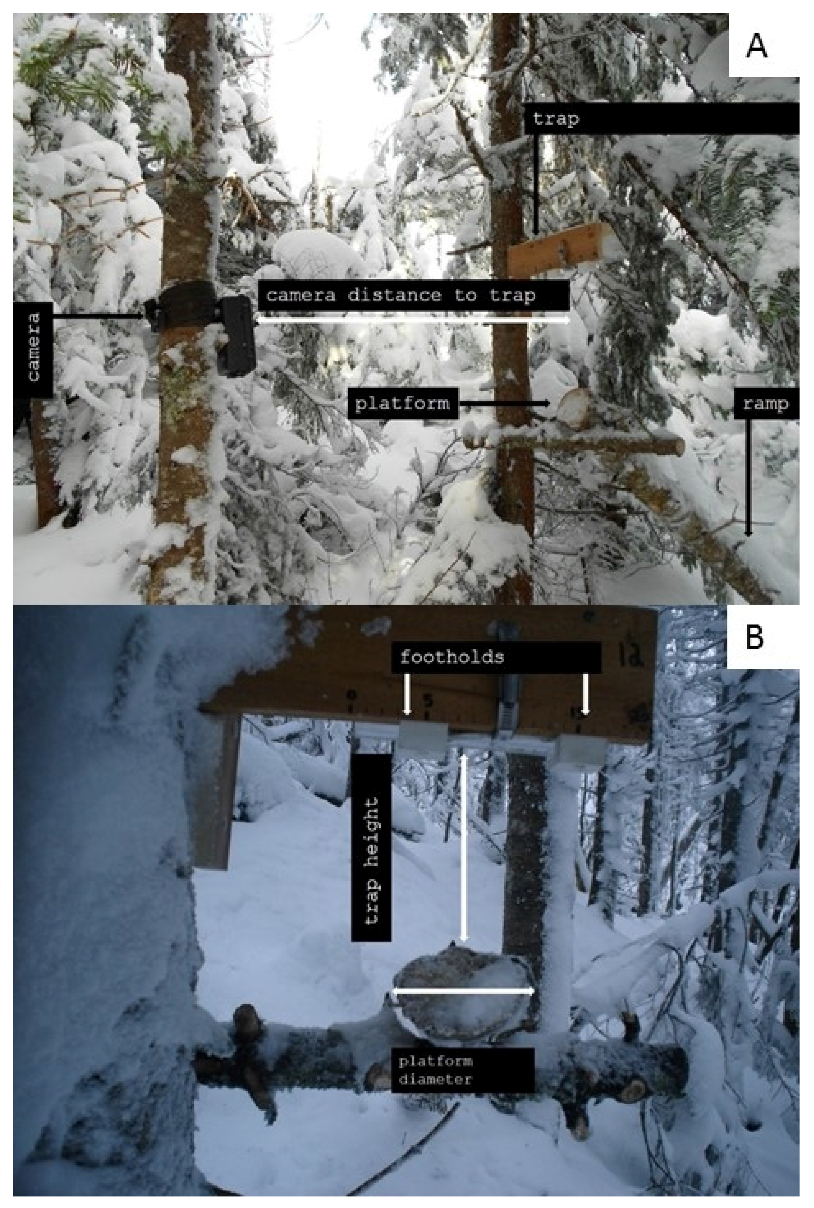
2.3. Camera-Trapping

We developed a camera-trap design over two winter field seasons (2011–2012) to photograph artificial markings placed on beacons of radio-collared martens and the ventral patches (throat and chest) of un-collared animals. We used four camera models (7 Bushnell Trophy Cam, Bushnell Corporation, Overland Park, KS, USA; three Moultrie GameSpy I-40, Moultrie Feeders, Alabaster, AL, USA, five Moultrie GameSpy I-45, Moultrie Feeders, Alabaster, AL, USA; and one custom built 4 MP game camera); all brand name cameras had passive infrared flashes and the custom built camera contained a white flash. We created custom flash filters for the infrared cameras because they were too bright for subjects closer than 1 m. To address the potential of detection bias originating from multiple camera brands [30], we set each camera brand/model to maximize capture (three continuous pictures or 5–15 s video and 1 min trigger reset for the Moultrie GameSpy cameras, three continuous pictures and 10 s trigger reset for the Bushnell Trophy Cam cameras, and one picture every 3 s for the custom camera).
The initial camera-trap design used in winter 2011 included a sardine can fastened to a tree branch/trunk, a leaning branch/log that allowed marten to access the bait, and a camera positioned ~1 m in front of the sardine can to view feeding marten. This approach performed reasonably well but the visibility of marten ventral patches was often compromised due to the positioning of the camera in relation to the sardines. For winter 2012, we attached customized baited traps to trees above the snow and positioned cameras on a post or tree 48–88 cm away from the trap (Figure 2A). We angled a 4–12 cm diameter log up to a supportive branch below each trap, and the trap height above the log varied 15–32 cm to determine a height that would best accommodate both sexes. Each trap was fitted with 3 cm wide footholds, and a bait corral that contained a 20 cm ruler (Figure 2B). The footholds allowed martens leverage to access bait, the bait corral kept the sardine can secure and forced marten to access the bait and reveal ventral patches, and the ruler was inscribed into the front of the trap to measure morphology with the intent of differentiating sex. Each trap was built identically to reduce variation, with spacing between footholds adjustable 6.4–10.2 cm. Hereafter and previously, we refer to the camera and the trap that contains the bait as the “camera-trap”.
The sex of un-collared martens was assigned by comparing morphological characteristics with radio-collared martens that visited the same camera-traps. Martens are sexually dimorphic; males have larger skull and body size [19,53], feet [54,55], and weigh nearly twice as much as females [18,54]. For 2011 we could only compare general differences (e.g., head morphology and body size; [19]) because camera-traps were unstandardized and had few measurement reference points (e.g., sardine can, tree limbs); in 2012 our camera-traps included a 20 cm measurement ruler and 3 cm wide footholds (Figure 3). Consequently, we used head and body morphology, and also front foot size to distinguish sex as male front feet were larger (n = 10, width = 3.0 ± 0.1 cm; n = 9, length = 3.5 ± 0.1 cm) than females (n = 9, width = 2.5 ± 0.1 cm; n =5, length = 3.0 ± 0.1 cm A. Siren, unpublished data), and martens readily used the 3 cm wide footholds. Generally, the front feet of males were as wide as or wider than the footholds, whereas female feet only spanned 3/4 of the foothold (Figure 3; LI = female, M15 = male).
Figure 2. Overview of camera-trap design (A) and components that were measured (A,B; white arrows) to determine the best configuration to capture marten ventral patterns.
Diversity 08 00003 g002
Figure 3. Ventral patches of seven collared (left; black font) and eight un-collared (right; white font) martens photographed during camera-trapping from 3–21 January 2012 in northern New Hampshire, USA. The id names of radio-collared martens were assigned during live capture (i.e., M1 = male #1 and F5 = female #5) and un-collared martens were assigned identities during the analysis of the photo-database. Note: Three of the un-collared martens were captured and radio-collared after winter 2012 camera-trapping and assigned ids (M13, M15, F14). Marten M7 in the upper left corner (shown in red boldface type) was captured in 2011, prior to the standardized design.
Diversity 08 00003 g003
The camera-trap line consisted of 30 sites for both winters; sites were chosen in a nonrandom pattern, spaced 637 ± 21 m (513–947) apart, baited with sardines, and a commercial skunk lure was used as an attractant. The average camera-trap density was 3.5 ± 0.8 traps/radio-collared marten home range (A. Sirén, unpublished data) which is above the suggested minimum [56]. We set camera-traps for 35 days (14 February–2 April) in winter 2011; three traplines of 10 traps were staggered to maximize trap density due to resource and time constraints and each trapline was set for 12 d (Figure 1). In winter 2012 camera-traps were set for 16 days (3–19 January), two traplines of 15 traps were staggered, and each trapline was set for 8 days (Figure 1). We shifted the location of two camera-trap sites in 2012 to increase tending efficiency (Figure 1). During both winters sites were visited midway to add bait, download pictures, and ensure cameras were working properly. Martens were often caught multiple times daily at the same camera-trap; these data were used to quantify the proportion of captures that were identifiable and collapsed into a single daily capture for camera SCR density analyses [42]. Individuals captured at different traps during the same day were not collapsed and used in the analyses.

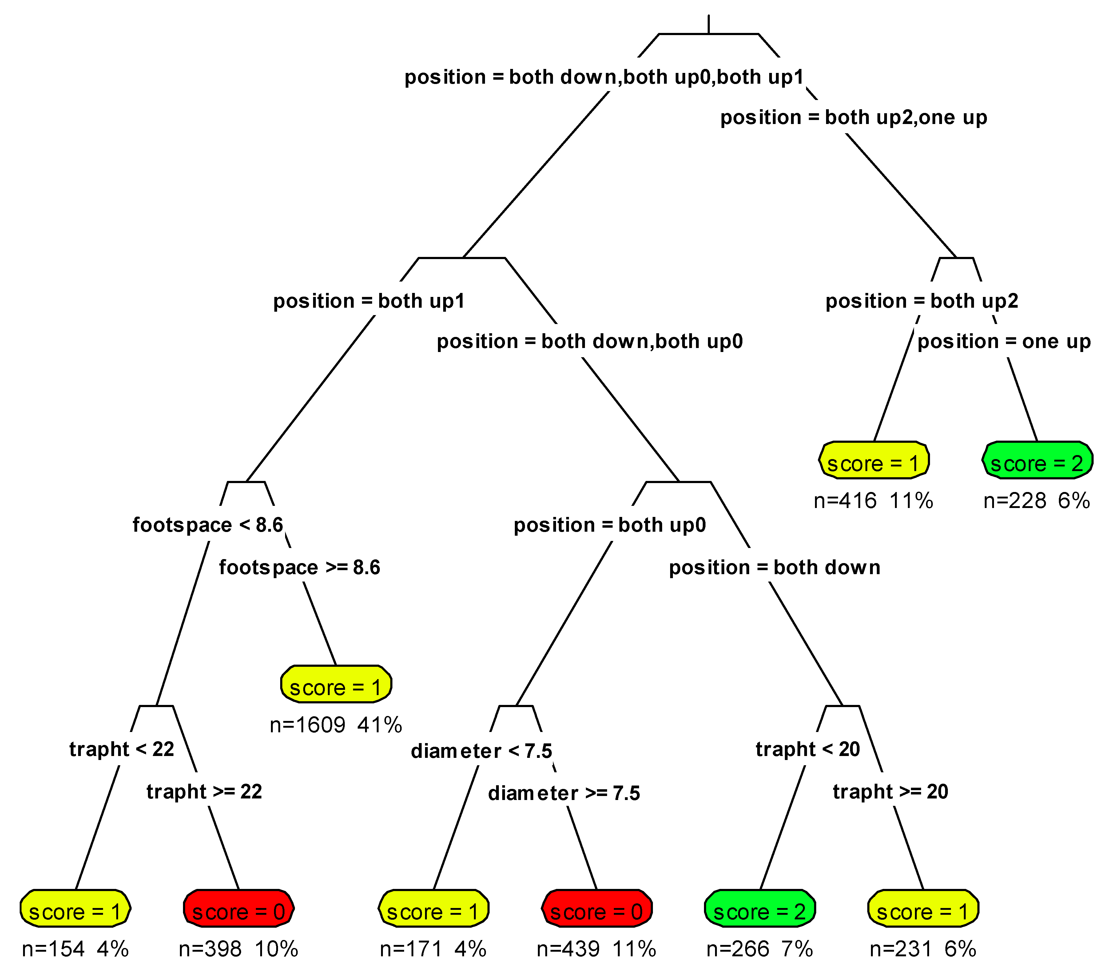
2.4. Ventral Scoring

We evaluated five different camera-trap parameters to determine the configuration and factors that maximized photo-capture of the ventral patterns of radio-collared martens. We only used data from 2012 because the camera-traps were standardized for this effort and therefore comparable. First, for each photo-capture of radio-collared martens we assigned a ventral score of the throat and chest patches: 0 = no marks visible; 1 = chest or throat patch visible; 2 = chest and throat patch visible. Second, we recorded foot positioning because preliminary tests revealed that positioning of martens influenced the visibility of ventral patches. Foot positioning was quantified as: both down = both feet below shoulder height; one up = one foot above shoulder height and the other below; both up0 = both feet above shoulder height but none touching footholds; bothup1 = both feet above shoulder height and one or both feet touching one foothold; bothup2 = both feet above shoulder height touching each foothold separately. Each observation of ventral scores and foot positioning included camera-trap parameters, including the camera distance from the trap, ramp diameter, trap height, and spacing between footholds. For example, the photograph of the radio-collared marten M1 in Figure 3 received a ventral score of “2”, and the foot positioning was “both down”. The trap was 48 cm from the camera, ramp diameter was 9 cm, the trap height was 15 cm from the ramp, and the foothold spacing was 7.6 cm.
We used classification and regression tree (CART) modeling to determine which parameters resulted in the highest ventral scores. CART modeling partitions a response variable based on the most influential fixed effects variable(s) [57]. Often several splits, or partitions, are performed to measure the contribution of predictor variables to a response [57]. We performed ordinal CART regression using the “rpartScore” package [58] in R statistical software [59]; ventral scores were treated as the ordinal response variable and foot positioning, trap height, camera distance, platform diameter, and foothold spacing were included as predictor variables.

2.5. Photographic Clusters

We used seven (5 M, 2 F) adult (>1 years) radio-collared martens monitored each winter (2011 and 2012), to evaluate temporal activity at camera-trap sites and define a threshold for temporal picture clusters (i.e., independent visits; [31]). Initially, we aggregated pictures by camera-trap sites into 1.25-min clusters as this cut-off point marked a drop between time intervals of consecutive pictures at each trap site. We also chose this cut-off because the Moultrie brand cameras could only take three images or one 5–30 s video per minute. We then organized pictures that were >1.25 min but <30 min apart that appeared to be a part of the same sequence, resulting in 138 and 80 clusters in for 2011 and 2012, respectively, which were considered independent captures of radio-collared martens. Each visit (min) and time between visits (min) at the same camera-trap was recorded for radio-collared martens in winters 2011–2012. We calculated the mean (±SE), median, and range of min for camera-trap visits and the interval between camera-trap visits at the same trap.

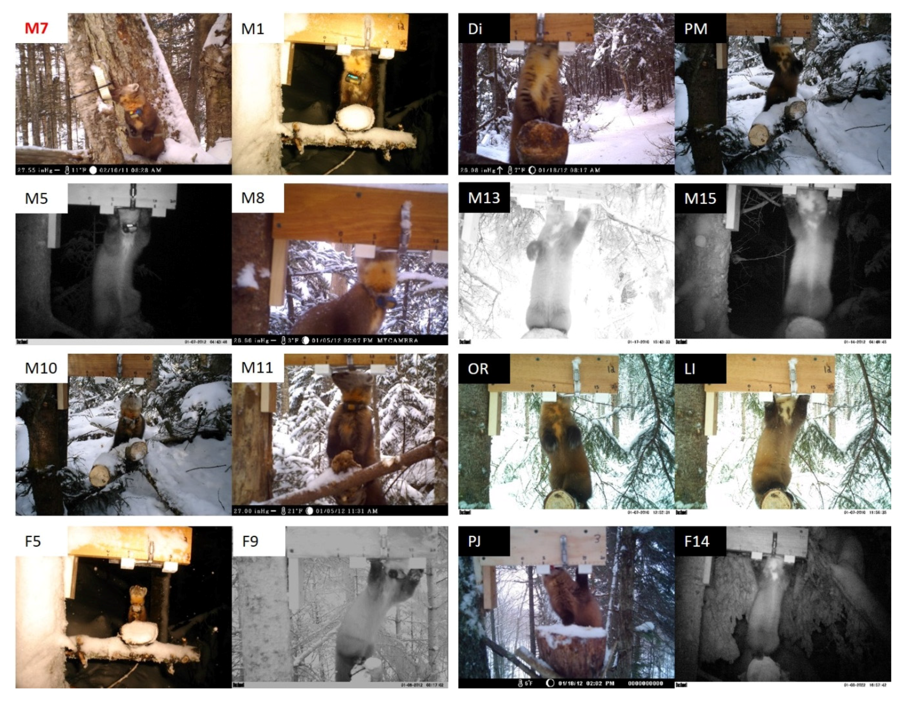
2.6. Identification of Un-Collared Martens

For winter 2012 data, we determined the number of un-collared martens, capture history, and proportion of unique captures that were identifiable by consensus of three observers (one co-author [O1] and two independent observers [O2, O3]). First, we organized the data into clusters based on the criteria determined for radio-collared martens (see Methods above) and only included pictures with high ventral scores within each cluster unless there were relatively few pictures. This process resulted in a photographic database of 60 temporal clusters containing a total of 357 photographs ( x - = 6 ± 1 cluster, range = 1–30). We then sent observers a protocol and the photographic database of un-collared martens, without any prior training. Observers were first instructed to evaluate whether each cluster contained 1 or >1 marten/cluster; for each picture observers would check “yes” to indicate that it was the same marten, “unsure” if they could not differentiate, and “no” if they thought it was another marten. They were then asked to name each un-collared marten within a cluster based on ventral characteristics (e.g., un-collared marten “Diamond” had a diamond shaped ventral pattern (Figure 3; “Di”)). The data from each observer were tallied, summarized, and cross-referenced with that of other observers. We calculated the proportion of identifiable and unidentifiable clusters that all three observers agreed upon, the proportion that were identifiable based on consensus (i.e., two of three observers agreed upon identity), and the total number of individuals based on consensus. To test for associations of cluster identity assignments between observers, we performed a Cramer’s V test [60] using the “vcd” R package [61] on all pairwise combinations (O1 and O2; O1 and O3; O2 and O3). This test measures the association between categorical data and provides a statistic that is equivalent to a correlation coefficient (−1 = perfect negative association, 0 = complete independence between samples, and 1 = perfect positive association).

2.7. Identification Probability

We were also interested in determining factors that influenced the ability of observers to assign identity to radio-collared and un-collared martens within picture clusters. Two co-authors assigned identities for both years and two independent observers participated in assigning identities for un-collared martens in 2012 (see Methods above). For each photographic cluster we recorded “identified” or “unidentified” and included seven covariates (cluster time, time since baiting, number of martens, camera brand/model, time of day, capture mode, year of camera-trapping) that we considered influential of identification probability. We hypothesized that longer camera-trap visits would increase identification probability and included the time of each cluster (min) as a covariate. We also considered the number of days that elapsed since camera-traps were baited (“elapse”) an influential factor that would decrease identification probability as repeated visits would reduce the amount of bait and therefore interest. Similarly, we thought that the number of martens that visited each camera-trap would also influence identification probability as more martens would consume the bait faster. Additionally, image quality of different cameras would influence our ability to identify martens so we included the camera brand/model as a model covariate. Similarly, we hypothesized that the time of day that martens visited traps would influence identification as cameras had different flash types (infrared and incandescent). We divided clusters into diel time periods (nocturnal, diurnal, and crepuscular), where crepuscular visits were defined as one hour prior to and after sunrise and sunset, and were calculated using the average local times for each month of the specific year. For those visits (i.e., clusters) that overlapped diel time periods, we assigned according to which period had the most use. The capture mode was also included (i.e., photo, video, or combined) as most cameras were set to take videos in 2011 and photos in 2012. Finally, because the camera-trap design was standardized for winter 2012, we felt that identification probability would be higher considering that martens would be consistently positioned in front of cameras; consequently, we included the year as a model covariate. Our primary hypothesis included two covariates and an interaction between the two (“min × elapse”) and were compared to two other interaction models (“martens × elapse”, “year × elapse”), a random intercept model (null hypothesis), and the univariate models listed above.
To identify influential parameters we used generalized linear mixed models (GLMM) with the logit link function using the “lme4” R package [62]. This package uses the Laplace approximation which is appropriate for hypothesis testing and ranking with a binary response [63]. Candidate models were ranked using Akaike’s Information Criterion for small sample size (AICc) with the “AICcmodavg” R package [64]. We considered models within two ∆AICc units to be comparable and evaluated the relative likelihood of the models using AICc weights (i.e., wi) [65]. We included each “trap” as a random intercept because contribution among camera-traps varied and the data contained repeated measures. The significance (P < 0.05) of the parameter estimates for the best fitting model was evaluated using Wald z-tests.

2.8. Camera- and Live-Capture SCR

Density analyses were performed using maximum likelihood estimation SCR software (”secr”; [66]) accessed in R [59]. First, the capture history and trap site locations for camera- and live-trapping efforts were tallied and stored in separate databases. For camera-trapping we used data from the 2011 and 2012 efforts described earlier. For live-trapping we used data from an effort that coincided with the end of camera-trapping in 2012 and lasted 6 days (17–22 January). Twenty-one live-traps were set at the camera-trap sites to compare SCR density estimates between camera- and live-trapping (Figure 1). This effort was shorter and fewer live-traps were deployed due to personnel and weather limitations; to compensate, live-traps were only set at camera-trap sites that were visited by martens during camera-trapping. See methods described earlier for live-trapping, immobilization, and handling.
We then created a spatial grid (i.e., habitat mask [2]) to measure the activity centers for individual marten during camera-and live-trapping to provide an estimate of density. The grid was created using Geographic Information System software (GIS; ArcGIS 10.1, ESRI, Redlands, CA, USA) and consisted of a minimum bounding rectangle that encompassed all trap locations to which a 3750 m buffer (3× the radius of an average marten home range) was added and equidistant sampling points (500 m) were included within the buffered rectangle using the Fishnet tool to achieve a density of 4 points/home range. The dimensions of the sampling grid and model parameters were chosen based on statistical considerations and marten spatial ecology [67]. Suitable and unsuitable habitat points within the grid were assigned a value of “1” and “0”, respectively; unsuitable habitat was considered to be early regenerating forest (0–20 years) and ponds as these are generally avoided by martens (see [68] for review).
In SCR, the capture probability for an individual i at a specific trap j is a function of the distance dij between that individual’s home range center and the trap location [69]. The home range centers are latent random variables estimated by the capture locations and parameters describing the detection function. Here, we used a half-normal detection function such that:
g(dij) = g0 exp(–dij2/2σ2)
The g0 parameter is the probability of detecting an individual during an occasion when it is located at its home range center. The likelihood of the observed captures was described by a Bernoulli encounter process for the camera data and a multinomial encounter process for the live-capture data. These specifications reflect differences in how individuals are captured by the “detectors” (i.e., cameras vs. live traps), since live-traps can only capture a single individual during a given occasion. We note that estimates of g0 can be biased when using a multi-catch likelihood for single-catch traps [69]. We evaluated three models that differed in their specification of g0 (null model M0, behavioral response (Mb), and animal × site learned response (Mbk)) using AICc model selection. The Mb and Mbk models were chosen and tested against a null model (M0) because marten often exhibit a behavioral response and would likely revisit baited traps. We considered sex-structured models but data were insufficient and early stages of model fitting suggested that differences were not supported by the data. We compared density estimates, corresponding measures of precision, and the movement parameter (σ) between camera- and live-trapping SCR from winter 2012. Because the camera SCR 2011 effort used the same trap locations it served as a replicate and was included to compare model selection and parameter estimates with winter 2012.

3. Results

3.1. Ventral Scoring

There were 3912 photos from the winter 2012 trapping effort available for the ventral scoring analysis to determine the optimal camera-trap configuration for capturing marten. The data were partitioned eight times, resulting in nine terminal nodes (Figure 4). Ventral scores were primarily associated with foot positioning and trap height, with some variance explained by foothold spacing and platform diameter (Figure 4). The highest scores (i.e., 2) occurred when martens were feeding at traps that were <20 cm above the feeding platform with both feet down (n = 266) or using one of the footholds to access bait (one up = 228, Figure 4). Intermediate scores (i.e., 1) were most associated with traps that had wider foot spacing (≥8.6 cm, n = 1609, Figure 4).

3.2. Photographic Clusters

There were 138 distinct photographic clusters of seven radio-collared martens during winter 2011 and 80 clusters of seven radio-collared martens during winter 2012. Martens visited camera-traps for 14 ± 2 min (11 ± 1 videos) in 2011 and 16 ± 3 min (84 ± 17 photos) in 2012; the median and range for both years was 7, and 1–104 min, respectively. There was no evidence that multiple martens were captured at the same camera-trap simultaneously; the mean time between visits at the same trap was 1532 ± 233 min (median = 419, range = 1–18,600) and visits <15 min by different martens at the same trap occurred infrequently (n = 3) for both years. The least time between visits at the same camera-trap by the opposite sex was 1 min, and the least time between visits of martens of the same sex was 6 min.
Figure 4. Classification and regression tree (CART) plot illustrating the influence of foot positioning (position), trap height (trapht), foothold spacing (footspace), and platform diameter (diameter) on ventral scores. Ventral scores are highlighted within each terminal node (0 = red, 1 = yellow, 2 = green), and the number of observations (n), and percent occurrence (%) for each node are listed directly below. The highest ventral scores (i.e., 2; green) were associated with traps that were spaced <20 cm above feeding platforms and when foot positioning was both down or one up. Note: See methods for a detailed description of foot positioning.
Diversity 08 00003 g004

3.3. Identification of Un-Collared Martens

Overall, the classification of un-collared martens by three observers was high and consistent. Observers never classified >1 marten within a photographic cluster, but were not always able to identify martens within the cluster. For example, O3 identified the marten in cluster #2 as “Double Heart” for 29 of the 30 pictures but could not identify it on the 28th picture of the cluster. O1 confirmed the identity of 94% (336 of 357) of the pictures within clusters, 22% of the clusters (13 of 60) contained at least one picture that was unidentifiable. Similarly, O2 confirmed the identity of 96% (341 of 357) of the pictures within clusters and 20% of the clusters (12 of 60) contained at least one picture that was unidentifiable. O3 identified fewer pictures overall (92%; 329 of 357) and had a higher number of clusters that contained at least one picture that was unidentifiable (27%; 16 of 60).
Observer O1 identified eight un-collared martens in 92% of the clusters (55 of 60), O2 identified eight un-collared martens in 95% of the clusters (57 of 60), and O3 identified nine individual martens in 78% of the clusters (47 of 60). The strength of association was high between all pairwise combinations of observers. The classification of identities was highest between O1 and O2 (Cramer’s V = 0.940); yet, association was still high between O1 and O3 (Cramer’s V = 0.869), and O2 and O3 (Cramer’s V = 0.862). The proportion of clusters that all three observers agreed upon (i.e., identifiable or unidentifiable) was 85% (51 of 60), the number agreed upon by consensus was 90% (54 of 60). In total, there were eight individual un-collared martens agreed upon by consensus. In addition to radio-collared individuals, we used the capture history of these martens to model identification probability and density.

3.4. Identification Probability

We used 230 and 156 photo clusters in winters 2011 and 2012, respectively, to determine factors that influenced the ability of observers to identify radio-collared and un-collared martens. The top identification probability model included two covariates and an interaction term (“min × elapse”), which was ∆AIC = −14.4 compared to the closest model “min” (see Supplementary Materials—Table S1). The ability of observers to identify martens was directly proportional to the length of time martens visited camera-traps (β = 0.143, P = 0.01), and inversely proportional to the number of days that the trap was baited (β = −0.344, P = 0.006; see Supplementary Materials—Table S2). Also, as the number of days since baiting elapsed, martens visited camera-traps for shorter periods reducing identification probability; however, this term was not significant (β = −0.018, P = 0.196; see Supplementary Materials—Table S2).

3.5. Camera- and Live-Capture SCR

In winter 2011 there were a total of 3130 files (1624 photos, 1506 videos) of radio-collared and un-collared marten during 35 occasions (i.e., trapping days). There were 230 recognizable captures (i.e., clusters), and marten were identifiable on 190 (83%) visits. In winter 2012 there were a total of 8948 photos of marten in 16 occasions. There were 156 recognizable captures and marten were identifiable on 134 (86%) visits.
During winter 2011, 13 martens were captured and recaptured at camera-traps, and in 2012, 14 of 15 martens were recaptured at camera-traps (Table 1). Radio-collared martens comprised approximately half of the sampled population during both years (n = 7; Appendix). For live-trapping in 2012, 10 of 15 martens were recaptured (Table 1), and six of these were radio-collared martens (Appendix). The sex ratio was approximately even (7M, 8F) and biased towards adults (13:2; Appendix). Mean capture probability (g0) for camera-trapping was 0.12 ± 0.03 for 2011 and 0.10 ± 0.03 for 2012, whereas g0 was higher and more variable for live-trapping (0.20 ± 0.26). Camera-trap failure was infrequent resulting in a 3% and 4% reduction in trap nights for winters 2011 and 2012, respectively, and live-trap failure was not recorded during winter 2012. Comparison of capture history between camera- and live-trapping was incomplete as four martens captured during live-trapping did not have ventral patches photographed during handling; minimally, there were nine radio-collared and un-collared martens captured during both efforts (Appendix).
Table 1. Associated density (D ± SE) of martens/km2, 95% confidence limits (CL) for top camera- and live-trap spatial capture–recapture (SCR) models. The proportion recaptured (% Recap), trap nights (TN), and catch-per-unit-effort (CPUE) are included for each capture effort.
Trapping Event aD ± SECL% RecapTNCPUE
Camera 20110.43 ± 0.120.25–0.75100% (13 of 13)33936 marten/100 TN
Camera 20120.60 ± 0.160.35–1.0193% (14 of 15)22438 marten/100 TN
Live-trap 20120.45 ± 0.240.16–1.2266% (10 of 15)11227 marten/100 TN
a The top camera-trap models for both years included a behavioral and a site learned response (i.e., Mbk). The top live-trap models were averaged as they shared similar AICc weights.
AICc model selection of camera SCR data for both years provided similar results; the top model was clearly the one which included a behavioral × site learned response (Table 2). However, for the live-trapping dataset all models shared weights; competing models were averaged to improve the precision of the density estimates (Table 2). For camera-trap SCR, density was estimated at 0.43, 0.25–0.75 martens/km2 in 2011 and 0.60, 0.35–1.01 martens/km2 in 2012. For live-trap SCR (2012), density was estimated at 0.45, 0.16–1.22 martens/km2. The movement parameter (i.e., σ) and level of precision were similar for both winters of camera-trapping (2011 = 818 ± 68 m; 2012 = 790 ± 81 m), whereas σ was higher and more variable for live-trapping (1173 ± 676 m; Figure 5).
Table 2. Model selection summary of camera- and live-trap SCR data over two winters in northern New Hampshire, USA. Models were evaluated using AICc, ranked using ∆AICc and model weight (wi).
Trapping EventModels akAICc∆AICcwi
Camera-trapping 2011modelbk4793.101
model03822.229.10
modelb4825.832.70
Camera-trapping 2012modelbk4573.901
model03605.631.70
modelb4606.332.50
Live-trapping 2012modelb4224.400.51
model03225.81.40.25
modelbk4225.91.60.23
a model0 = no behavioral response; modelb = behavioral response; and modelbk = animal × site learned response.
Figure 5. Mean (± SE) σ values (m) from SCR density estimates, and mean (± SE) 95% MCP home range radius (m) for male, female, and sub-dominant male radio-collared martens over two winters of camera- and live-trapping, and radio telemetry monitoring. Note: Sample size is listed above SE bars.
Diversity 08 00003 g005

4. Discussion

Our results show that optimal spatial configuration and temporal clustering of photographs can have a substantial effect on the identification of individual animals. Ventral scores were greatly improved when the front feet of martens were either both down on the platform or positioned in a manner that allowed the ventral patches to be photographed (e.g., one up). The foot positioning was influenced by trap position, with higher scores when traps were 15–20 cm above the platform due to optimized capture of ventral patches. Although sample size of female martens was small, those visiting traps within this range had higher ventral scores than those visiting traps spaced higher above the platform. The use of footholds provided equivocal results; while wider spacing provided leverage to access bait, the front feet would sometimes block ventral patches. Although camera distance was not an influential factor, ventral marks were most visible when cameras were at an intermediate distance (48–68 cm) to the trap. We suggest incorporating the camera and trap within a partially or fully closed design and use a single brand incandescent flash camera, as martens did not appear to be trap-shy and this camera type provided the best images. Importantly, reducing variability of equipment and light conditions increases the ability of automated computer identification systems [40,70].
Temporal clustering of photographs had a positive effect on probability of identification as well. We quantified camera-trap visits of radio-collared martens and documented long visits, providing ample opportunity for capturing ventral patches for photo identification. Importantly, simultaneous visits (i.e., more than one marten visiting the trap at the same time) were never documented and visits by different martens at the same camera-trap were typically spaced >15 min which was higher than the threshold delineated for clustered photographs of the same individual (1.25 min). Similarly, although the identity of a marten could not always be confirmed, observers never assigned >1 marten within a cluster, corroborating visitation patterns of telemetered individuals at camera-traps. Previous studies have either used field data to assign independent observations (e.g., >3 min between consecutive bobcat (Lynx rufus) pictures; [31]) or by using recommendations from the literature (e.g., [9,32]). However, what constitutes an independent visit for one species may not be applicable to others. We recommend future studies quantify camera-trap visits to determine species-specific cut-off points. This is especially relevant for baited designs that result in large photographic databases and require considerable pre-processing prior to the identification process (independent observers or automated software).
The proportion of un-collared martens we identified is considered high for camera-trap studies [29,37,71,72]. We had similar agreement of the number of martens identified (O1 = 8, O2 = 8, O3 = 9) and the proportion of martens that were identifiable and not identifiable within clusters. The two independent observers also reported that viewing clustered photographs increased their ability to identify martens in other clusters due to multiple views of marten ventral patches. Using clustered photographs of marten was a significant improvement compared to using one picture/video to identify marten (36%), and it increased the efficiency of classifiers to identify individuals and create a capture history (~4 h) compared to using single files alone (~40 h; A. Siren, unpublished data). We believe that this process contributed to the high agreement of capture history among observers and suggest using this approach for other species with distinct pelage characteristics or morphological traits.
Similarly, we determined several factors that influenced the ability of observers to identify martens. As predicted, the identification probability was directly proportional to the length of time martens visited camera-traps, inversely proportional to the number of days since traps were baited, and martens visited traps less often as the number of days increased since baiting, indicating a behavioral response to an empty bait can. These results indicate that identification probability can be controlled by ensuring that camera-traps are rebaited at short intervals. In 2012 camera-traps were rebaited approximately once every 4 days, whereas they were only checked and rebaited once weekly in 2011. Although not significant, identification probability remained higher with a 4-day tend compared to every 7 days; the tending schedule may need to be modified if marten density is higher. We included the number of martens that visited each camera-trap as a proxy for density and although there was weak support for this model, it is plausible that when more martens are present bait will be consumed quicker. However, the territorial behavior of martens may prevent subordinate individuals from accessing bait, except potentially when resources are particularly abundant [73].
While the identification of individuals is achievable, the ability to correctly classify the sex and distinguish between juvenile and adults increases the complexity. Differentiating sex is easier to accomplish with dimorphic species such as martens and was attempted in this study. Our method might be improved by widening the capture zone to include the genital area as was done with wolverines (Gulo gulo) in Alaska [8]; however, it should not compromise the identification of ventral patches. Using landmarks that are readily captured and in close proximity to the ventral patches may be more practical for distinguishing sex (e.g., head and front feet). For example, male martens have wider and longer skulls than females [19,53], and combined with front foot morphology may increase classification. Providing a ruler to make comparisons is important, and may be integrated with photo analysis software to provide quantitative comparisons of morphology. Thompson [74] used the ratio of head morphology and camera-trap landmarks (ear-width/treadle width) to classify the gender of fisher and correctly classified 82.5% of known males and 94.7% of known females. While identification of sex is possible, the greatest challenge is to distinguish juvenile and adult marten because they reach adult size their first winter.
This study featured a rare comparison between camera- and live-trapping using a sample of radio-collared and un-collared individuals. Model selection, and parameter estimates for both years of camera-trapping were alike; the top models for both years included a behavioral × site learned response. This is unsurprising as marten are a territorial species and respond positively to baited camera-traps after the initial detection [55,75,76], similar to wolverines [77]. Although, density was higher during winter 2012, capture probability and σ were similar in both winters, providing evidence that camera-trapping provided a relatively unbiased estimate of marten spacing and movement patterns. The latter statistic (i.e., σ) was similar to the average home range radius of telemetered marten with males having larger home ranges (Figure 5). Interestingly, precision was greater for all parameter estimates for winter 2011, likely attributed to increased effort and sample size. This is expected as non-invasive methods such as camera-trapping [15] and genetic tagging [13] provide robust sampling which can improve parameter estimation and precision.
Comparatively, live-trapping density for winter 2012 was lower and less precise compared to camera SCR and the σ value was considerably higher compared to both years of camera-trapping (Figure 5). This was likely due to reduced effort and a lower recapture rate. Further, AICc model selection of live-trapping data indicated that sample size was likely too small, as the null model performed as well as those which included behavioral and trap specific responses (Table 2). Although SCR models can deal with sparse datasets it is advisable to have ≥20 recaptures [41], 33% more than in this study (n = 15). However, if ancillary data is available (as in this study), combining multiple data sources can improve parameter estimation and the precision of density estimates [78,79]. Although we consider our live-trapping density estimates to be biased, both methods (i.e., camera- and live-trapping) were within the range of previous studies that used genetic data [76], live-trapping [80], and radio-telemetry [23].
While trap shyness is common for live-trapping, it has also been documented in camera-trap studies (e.g., [81,82,83]) due to camera flash. Martens are very tolerant of camera flash as our data suggests; however, trap shyness is common for martens in live-trapping studies [84]. For traditional capture mark-recapture modeling, trap shyness creates negative bias toward capture probability and positive bias toward abundance when using a null model which assumes no behavioral response [33]. When there are sufficient data, this behavioral response can be accounted for and appropriately modeled; however, when effort and sampling are reduced, behavioral responses might remain undetected resulting in biased estimates of detection probability and density [15]. For SCR models, small sample size and/or biased recaptures might produce the opposite trend compared to traditional CMR models [45]. For example, when recaptures are sparse and biased towards individuals that exhibit different space use, the mean movement parameter will be skewed [45]. This pattern was observed for black bears where male movements were overestimated leading to underestimated density [45]. Similarly, the movement parameter (i.e., σ) was high for live-trapping compared to both years of camera-trapping in our study (Figure 5) and attributed to two males that were caught most often during live-trapping (Appendix) and had the longest movements. Further, several marten (especially females) became trap shy during live-trapping and this likely contributed towards fewer and biased recapture (Appendix). We posit that this dynamic contributed to our negatively biased density estimate. Further, because live-traps are single catch devices that limit capture opportunities compared to camera-traps, this greatly reduced the sampling opportunity.
Understanding the degree to which study animals exhibit a behavioral response can be difficult to determine, especially when sample size is low and cannot be explicitly incorporated in model evaluation. Considering that minimally invasive survey techniques often have low sample size and lack demographic data, the potential for biased density estimates may occur at a greater likelihood. Also, because SCR is increasingly used to reanalyze existing live- trapping datasets, it is important to identify potential behavioral responses. Although effort was minimal for live-trapping in this study, it was comparable to previously published studies that used live-trapping to estimate marten density (e.g., [22,80,85,86]). Further, the spatial ecology of a species may vary by sex and age influencing capture heterogeneity as well. These potential problems provide further support to develop sampling techniques that provide demographic information on captured individuals. While the identity of sex is plausible using camera-trapping (see [8]) and was estimated in this study, it may be difficult to reliably determine the age of an individual. However, recent genetic methods to determine age (e.g., [87]) might work well in tandem with camera-trapping and provide important covariates to be included in SCR density estimation.

5. Conclusions

Our camera-trap method allowed us to identify individual martens using unique ventral patterns. We determined a camera-trap configuration that increased capture of marten ventral patterns and recorded long and non-overlapping visits by martens, providing ample opportunity to identify individuals. These factors likely contributed to the mutual agreement of capture history among observers. Importantly, we also determined factors that influenced the ability of observers to identify martens. The length of time martens visited traps and the time that elapsed since traps were baited influenced our ability to identify martens. This study provides evidence that camera-trapping provides relatively unbiased estimates of density compared to traditional live-trapping, due to increased recapture rates and reduced behavioral response. While we encourage researchers to adopt the camera-trap method and improve upon it, we also caution those using SCR modeling for live-trap datasets. Although recent modeling approaches may effectively handle smaller sample sizes (e.g., Bayesian SCR; [45]), capture–recapture modeling—traditional or SCR—still requires larger sample sizes to reduce bias and increase precision.

Supplementary Materials

The following are available online at www.mdpi.com/1424-2818/8/1/3/s1, Table S1: GLMM describing identification probability of American martens at camera traps from 14 February–2 April 2011 and 3–19 January 2012 in northern New Hampshire, USA. Models were evaluated using AICc, ranked using ∆AICc and model weight (wi), Table S2: Primer sequences used in this study. Parameter estimates and associated standard errors (SE), Wald’s z-values, and probability statistics that influenced identification probability of American martens at camera traps. Note: parameters in boldface type are significant.

Acknowledgments

Funding for this project was provided through NH Wildlife Restoration program grant W-97-R-1 in cooperation with the U.S. Fish and Wildlife Service, Wildlife and Sport Fish Restoration Program. Additional support was provided by the Department of Interior, Northeast Climate Science Center. We would like to thank Wagner Forest Management, American Forest Management, and lessee Brookfield Renewable Power for providing access to the study site. The New Hampshire Fish and Game Department, United States Fish and Wildlife Service, and Stantec Environmental Consultants provided invaluable assistance, equipment, and lodging. Jill Kilborn, Will Staats, Andy Timmins, Henry Jones, and Jackie Comeau provided invaluable field assistance. We especially thank the two anonymous photographic observers for their contribution. We also thank Dan Linden, John Clare, John Litvaitis, and ToniLyn Morelli for reviewing the manuscript in its early stages.

Author Contributions

This study was co-designed and implemented by Alexej P. K. Sirén as part of his MSc. thesis at the University of New Hampshire, USA. Peter J. Pekins, his advisor, assisted with study design and manuscript writing. Peter L. Abdu assisted with camera-trap design, field efforts during winter 2012, and photographic database management and analysis. Mark J. Ducey provided statistical support and assisted with manuscript writing.

Conflicts of Interest

The authors declare no conflict of interest.

Appendix

Appendix: The sex (S), age (A), number of recaptures (rec), and number of different traps visited (trap) for radio-collared and un-collared marten over two winters of camera- and live-trapping in northern New Hampshire, USA.
Live-Trapping 2012Camera-Trapping 2012Camera-Trapping 2011
Id aS bA crectrapId aS bA crectrapId aS bA crectrap
F10FJ01Un1M-12Un1F-32
F11FA01Un2F-22Un2M-33
F12FA01Un3F-11Un3F-12
F13FA12Un4M-55Un4F-11
F14FA11Un5F-12F4FA52
F15FA01F14 **FA01F5FA75
F5FA11F5FA12F7 **FA116
F9FA21F9FA82M1MA114
M1 *MA23M1MA177M2 **MA63
M10MA22M10MA53M3MA217
M11MA01M11MA43M5MA2810
M12MA01M13 **MA83M6MJ12
M13 *MJ44M15 **MA82M7MA135
M14MA11M5MA86
M8MA11M8MA22
a Radio-collared and/or ear-tagged martens were given an id based on sex (e.g., M1 denotes the first male and F10 represents the 10th female caught during the study). Martens captured only during camera-trapping were given the id “Un”, unless ventral patterns were recognizable during subsequent live-capture efforts. b Sex was determined by physical examination during live-capture. For camera-trapping, sex was assigned for un-collared martens in winter 2012, by comparing morphological characteristics (see description in methods). c Age was determined either by cementum analysis from recovered mortalities or palpation of cranial ridge (males only) and examination of tooth wear during capture. Age for un-collared marten was not estimated and this is denoted by a hyphen. * Contributed to biased σ due higher recaptures and longer movements. ** Assigned identification numbers after comparing pictures of throat patches taken during camera-trapping with those taken during capture and handling.

References

  1. Seber, G.A.F. Estimation of Animal Abundance and Related Parameters, 2nd ed.; Macmillan: New York, NY, USA, 1982. [Google Scholar]
  2. Efford, M. Density estimation in live-trapping studies. Oikos 2004, 106, 598–610. [Google Scholar] [CrossRef]
  3. Jhala, Y.V.; Mukherjee, S.; Shah, N.; Chauhan, K.S.; Dave, C.V.; Meena, V.; Banerjee, K. Home range and habitat preference of female lions (Panthera leo persica) in Gir forests, India. Biodivers. Conserv. 2009, 18, 3383–3394. [Google Scholar] [CrossRef]
  4. O’Connell, A.F.; Nichols, J.D.; Karanth, K.U. Introduction. In Camera Traps in Animal Ecology: Methods and Analyses; O’Connell, A.F., Nichols, J.D., Karanth, K.U., Eds.; Springer Science and Business Media: New York, NY, USA, 2011; pp. 1–8. [Google Scholar]
  5. Pollock, K.H.; Nichols, J.D.; Brownie, C.; Hines, J.E. Statistical inference for capture-recapture experiments. Wildl. Monogr. 1990, 107, 3–97. [Google Scholar]
  6. Noyce, K.V.; Garshelis, D.L.; Coy, P.L. Differential vulnerability of black bears to trap and camera sampling and resulting biases in mark-recapture estimates. Ursus 2001, 12, 211–225. [Google Scholar]
  7. Karanth, K.U.; Nichols, J.D. Estimation of tiger densities in India using photographic captures and recaptures. Ecology 1998, 79, 2852–2862. [Google Scholar] [CrossRef]
  8. Magoun, A.J.; Long, C.D.; Schwartz, M.K.; Pilgrim, K.L.; Lowell, R.E.; Valkenburg, P. Integrating motion-detection cameras and hair snags for wolverine identification. J. Wildl. Manag. 2011, 75, 731–739. [Google Scholar] [CrossRef]
  9. Negrões, N.; Sarmento, P.; Cruz, J.; Eira, C.; Revilla, E.; Fonseca, C.; Sollmann, R.; Torres, N.M.; Furtado, M.M.; Jacoma, A.T.A.; et al. Use of camera-trapping to estimate puma density and influencing factors in central Brazil. J. Wildl. Manag. 2010, 74, 1195–1203. [Google Scholar] [CrossRef]
  10. Goswami, V.R.; Lauretta, M.V.; Madhusudan, M.D.; Karanth, K.U. Optimizing individual identification and survey effort for photographic capture–recapture sampling of species with temporally variable morphological traits. Anim. Conserv. 2012, 15, 174–183. [Google Scholar] [CrossRef]
  11. Hebeisen, C.; Fattebert, J.; Baubet, E.; Fischer, C. Estimating wild boar (Sus scrofa) abundance and density using capture–resights in Canton of Geneva, Switzerland. Eur. J. Wildl. Res. 2008, 54, 391–401. [Google Scholar] [CrossRef]
  12. Alonso, R.S.; McClintock, B.T.; Lyren, L.M.; Boydston, E.E.; Crooks, K.R. Mark-recapture and mark-resight methods for estimating abundance with remote cameras: A carnivore case study. PLoS ONE 2015, 10, e0123032. [Google Scholar] [CrossRef] [PubMed]
  13. Lukacs, P.M.; Burnham, K.P. Review of capture–recapture methods applicable to noninvasive genetic sampling. Mol. Ecol. 2005, 14, 3909–3919. [Google Scholar] [CrossRef] [PubMed]
  14. Waits, L.P.; Paetkau, D. Noninvasive genetic sampling tools for wildlife biologists: A review of applications and recommendations for accurate data collection. J. Wildl. Manag. 2005, 69, 1419–1433. [Google Scholar] [CrossRef]
  15. Foster, R.J.; Harmsen, B.J. A critique of density estimation from camera-trap data. J. Wildl. Manag. 2012, 76, 224–236. [Google Scholar] [CrossRef]
  16. Powell, R.A.; Buskirk, S.W.; Zielinski, W.J. Fisher (Martes pennanti) and marten (Martes americana). In Wild Mammals of North America: Biology, Management, and Conservation, 2nd ed.; Feldhamer, G., Thompson, B.C., Chapman, J.A., Eds.; Johns Hopkins University Press: Baltimore, MD, USA, 2003; pp. 635–649. [Google Scholar]
  17. Chapin, T.G.; Harrison, D.J.; Phillips, D.M. Seasonal habitat selection by marten in an untrapped forest preserve. J. Wildl. Manag. 1997, 61, 707–717. [Google Scholar] [CrossRef]
  18. Buskirk, S.W.; McDonald, L.L. Analysis of variability in home-range size of the American marten. J. Wildl. Manag. 1989, 53, 997–1004. [Google Scholar] [CrossRef]
  19. Yom-Tov, Y.; Yom-Tov, S.; Jarrell, G. Recent increase in body size of the American marten Martes americana in Alaska. Biol. J. Linn. Soc. 2008, 93, 701–707. [Google Scholar] [CrossRef]
  20. Long, R.A.; Mackay, P. Noninvasive methods for surveying martens, sables, and fishers. In Biology and Conservation of Martens, Sables, and Fishers: A New Synthesis; Aubry, K.B., Zielinski, W.J., Raphael, M.G., Proulx, G., Buskirk, S.W., Eds.; Comstock Pub. Associates: Ithaca, NY, USA, 2012; pp. 320–342. [Google Scholar]
  21. Chapin, T.G.; Harrison, D.J.; Katnik, D.D. Influence of landscape pattern on habitat use by American marten in an industrial forest. Conserv. Biol. 1998, 12, 96–227. [Google Scholar] [CrossRef]
  22. Hargis, C.D.; Bissonette, J.; Turner, D.L. The influence of forest fragmentation and landscape pattern on American martens. J. Appl. Ecol. 1999, 36, 157–172. [Google Scholar] [CrossRef]
  23. Poole, K.G.; Porter, A.D.; Vries, A.D.; Maundrell, C.; Grindal, S.D.; St. Clair, C.C. Suitability of a young deciduous-dominated forest for American marten and the effects of forest removal. Can. J. Zool. 2004, 82, 423–435. [Google Scholar] [CrossRef]
  24. Carroll, C. Interacting effects of climate change, landscape conversion, and harvest on carnivore populations at the range margin: Marten and lynx in the northern Appalachians. Conserv. Biol. 2007, 21, 1092–1104. [Google Scholar] [CrossRef] [PubMed]
  25. Lawler, J.J.; Safford, H.D.; Girvetz, E.H. Martens and fishers in a changing climate. In Biology and Conservation of Martens, Sables, and Fishers: A New Synthesis; Aubry, K.B., Zielinski, W.J., Raphael, M.G., Proulx, G., Buskirk, S.W., Eds.; Comstock Pub. Associates: Ithaca, NY, USA, 2012; pp. 371–397. [Google Scholar]
  26. De Bondi, N.; White, J.G.; Stevens, M.; Cooke, R. A comparison of the effectiveness of camera trapping and live trapping for sampling terrestrial small-mammal communities. Wildl. Res. 2010, 37, 456–465. [Google Scholar] [CrossRef]
  27. Villette, P.; Krebs, C.J.; Jung, T.S.; Boonstra, R. Can camera trapping provide accurate estimates of small mammal (Myodes rutilus and Peromyscus maniculatus) density in the boreal forest? J. Mammal. 2015. [Google Scholar] [CrossRef]
  28. Kays, R.W.; Slauson, K.M. Remote cameras. In Noninvasive Survey Methods for Carnivores; Long, R.A., MacKay, P., Zielinski, W.J., Ray, J.C., Eds.; Island Press: Washington, DC, USA, 2008; pp. 111–140. [Google Scholar]
  29. Kelly, M.J.; Noss, A.J.; di Bitetti, M.S.; Maffei, L.; Arispe, R.L.; Paviolo, A.; de Angelo, C.D.; di Blanco, Y.E. Estimating puma densities from camera trapping across three study sites: Bolivia, Argentina, and Belize. J. Mammal. 2008, 89, 408–418. [Google Scholar] [CrossRef]
  30. Wellington, K.; Bottom, C.; Merrill, C.; Litvaitis, J.A. Identifying performance differences among trail cameras used to monitor forest mammals. Wildl. Soc. Bull. 2014, 38, 634–638. [Google Scholar] [CrossRef]
  31. Mendoza, E.; Martineau, P.R.; Brenner, E.; Dirzo, R. A novel method to improve individual animal identification based on camera-trapping data. J. Wildl. Manag. 2011, 75, 973–979. [Google Scholar] [CrossRef]
  32. Gerber, B.D.; Karpanty, S.M.; Kelly, M.J. Evaluating the potential biases in carnivore capture–recapture studies associated with the use of lure and varying density estimation techniques using photographic-sampling data of the Malagasy civet. Popul. Ecol. 2012, 54, 43–54. [Google Scholar] [CrossRef]
  33. Otis, D.L.; Burnham, K.P.; White, G.C.; Anderson, D.R. Statistical inference from capture data on closed animal populations. Wildl. Monogr. 1978, 62, 1–135. [Google Scholar]
  34. Link, W.A.; Yoshizaki, J.; Bailey, L.L.; Pollock, K.H. Uncovering a latent multinomial: Analysis of mark–recapture data with misidentification. Biometrics 2010, 66, 178–185. [Google Scholar] [CrossRef] [PubMed]
  35. Chandler, R.B.; Royle, J.A. Spatially explicit models for inference about density in unmarked or partially marked populations. Ann. Appl. Stat. 2013, 7, 936–954. [Google Scholar] [CrossRef]
  36. Oliveira-Santos, L.G.R.; Zucco, C.A.; Antunes, P.C.; Crawshaw, P.G. Is it possible to individually identify mammals with no natural markings using camera-traps? A controlled case-study with lowland tapirs. Mamm. Biol. 2010, 75, 375–378. [Google Scholar] [CrossRef]
  37. Clare, J.D.; Anderson, E.M.; MacFarland, D.M. Predicting bobcat abundance at a landscape scale and evaluating occupancy as a density index in central Wisconsin. J. Wildl. Manag. 2015, 79, 469–480. [Google Scholar] [CrossRef]
  38. Kelly, M.J. Computer-aided photograph matching in studies using individual identification: An example from Serengeti cheetahs. J. Mammal. 2001, 82, 440–449. [Google Scholar] [CrossRef]
  39. Anderson, C.J.; Lobo, N.D.V.; Roth, J.D.; Waterman, J.M. Computer-aided photo-identification system with an application to polar bears based on whisker spot patterns. J. Mammal. 2010, 91, 1350–1359. [Google Scholar] [CrossRef]
  40. Allen, W.L.; Cuthill, I.C.; Scott-Samuel, N.E.; Baddeley, R. Why the leopard got its spots: Relating pattern development to ecology in felids. Proc. R. Soc. B Biol. Sci. 2010, 278, 1373–1380. [Google Scholar] [CrossRef] [PubMed]
  41. Efford, M.G.; Borchers, D.L.; Byrom, A.E. Density estimation by spatially explicit capture–recapture: Likelihood-based methods. In Modeling Demographic Processes in Marked Populations; Thomson, D.L., Cooch, E.G., Conroy, M.J., Eds.; Springer US: New York, NY, USA, 2009; pp. 255–269. [Google Scholar]
  42. Royle, J.A.; Karanth, K.U.; Gopalaswamy, A.M.; Kumar, N.S. Bayesian inference in camera trapping studies for a class of spatial capture-recapture models. Ecology 2009, 90, 3233–3244. [Google Scholar] [CrossRef] [PubMed]
  43. Wilson, K.R.; Anderson, D.R. Evaluation of two density estimators of small mammal population size. J. Mammal. 1985, 66, 13–21. [Google Scholar] [CrossRef]
  44. Obbard, M.E.; Howe, E.J.; Kyle, C.J. Empirical comparison of density estimators for large carnivores. J. Appl. Ecol. 2010, 47, 76–84. [Google Scholar] [CrossRef]
  45. Sollmann, R.; Gardner, B.; Belant, J.L. How does spatial study design influence density estimates from spatial capture-recapture models? PLoS ONE 2012, 7, e34575. [Google Scholar] [CrossRef] [PubMed]
  46. Ivan, J.S.; White, G.C.; Shenk, T.M. Using auxiliary telemetry information to estimate animal density from capture-recapture data. Ecology 2013, 94, 809–816. [Google Scholar] [CrossRef]
  47. Gardner, B.; Reppucci, J.; Lucherini, M.; Royle, J.A. Spatially explicit inference for open populations: Estimating demographic parameters from camera-trap studies. Ecology 2010, 91, 3376–3383. [Google Scholar] [CrossRef] [PubMed]
  48. Solberg, K.H.; Bellemain, E.; Drageset, O.M.; Taberlet, P.; Swenson, J.E. An evaluation of field and non-invasive genetic methods to estimate brown bear (Ursus arctos) population size. Biol. Conserv. 2006, 128, 158–168. [Google Scholar] [CrossRef]
  49. Davis, M.; Gratton, L.; Adams, J.; Goltz, J.; Stewart, C.; Buttrick, S.; Zinger, N.; Kavanagh, K.; Sims, M.; Mann, G. New England-Acadian Forests. Available online: http://worldwildlife.org/ecoregions/na0410/ (accessed on 21 November 2013).
  50. McNab, W.H.; Avers, P.E. Ecoregions and Subregions of the United States: Section Descriptions; USDA Forest Service Administrative Publication WO-WSA-5; USDA Forest Service: Washington, DC, USA, 1994. [Google Scholar]
  51. Sirén, A.P.; Pekins, P.J.; Ducey, M.J.; Kilborn, J.R. Spatial ecology and resource selection of a high elevation American marten population in the northeastern United States. Can. J. Zool. 2015. [Google Scholar] [CrossRef]
  52. Bull, E.L.; Heater, T.W.; Culver, F.G. Live-trapping and immobilizing American martens. Wildl. Soc. Bull. 1996, 24, 555–558. [Google Scholar]
  53. Poole, K.G.; Matson, G.M.; Strickland, M.A.; Magoun, A.J.; Graf, R.P.; Dix, L.M. Age and sex determination for American martens and fishers. In Martens, Fishers, and Sables: Biology and Conservation; Buskirk, S.W., Harestad, A.S., Raphael, M.G., Powell, R.A., Eds.; Cornell Univ. Press: Ithaca, NY, USA, 1994; pp. 204–223. [Google Scholar]
  54. Krohn, W.B.; Hoving, C.; Harrison, D.; Phillips, D.; Frost, H. Martes foot-loading and snowfall patterns in eastern North America: Implications to broad-scale distributions and interactions of mesocarnivores. In Martens and Fishers (Martes) in Human-Altered Environments; Harrison, D.J., Fuller, A.K., Proulx, G., Eds.; Springer Science and Business Media, Inc.: New York, NY, USA, 2004; pp. 115–131. [Google Scholar]
  55. Slauson, K.M.; Truex, R.L.; Zielinski, W.J. Determining the gender of American martens and fishers at track plate stations. Northwest Sci. 2008, 82, 185–198. [Google Scholar] [CrossRef]
  56. Dillon, A.; Kelly, M.J. Ocelot Leopardus pardalis in Belize: The impact of trap spacing and distance moved on density estimates. Oryx 2007, 41, 469–477. [Google Scholar] [CrossRef]
  57. Breiman, L.; Friedman, J.H.; Olshen, R.A.; Stone, C.J. Classification and Regression Trees; Wadsworth: Belmont, MA, USA, 1984. [Google Scholar]
  58. Galimberti, G.; Soffritti, G.; di Maso, M. Classification Trees for Ordinal Responses in R: The rpartScore Package. J. Stat. Softw. 2012, 47, 1–25. [Google Scholar] [CrossRef]
  59. R Development Core Team. R: A language and environment for statistical computing; R Foundation for Statistical Computing, Vienna, Austria; Available online: http://www.R-project.org/ (accessed on 2 July 2015).
  60. Kendall, M.; Stuart, A. The Advanced Theory of Statistics; Macmillan: New York, NY, USA, 1979; Volume 2. [Google Scholar]
  61. Meyer, D.; Zeileis, A.; Hornik, K. Vcd: Visualizing Categorical Data. R Package Version 1.4-1. Available online: https://cran.r-project.org/web/packages/vcd (accessed on 15 July 2015).
  62. Bates, D.; Maechler, M.; Bolker, B.; Walker, S. lme4: Linear Mixed-Effects Models Using Eigen and S4. R Package Version 1.1-7. Available online: https://cran.r-project.org/web/packages/lme4 (accessed on 10 November 2014).
  63. Bolker, B.M.; Brooks, M.E.; Clark, C.J.; Geange, S.W.; Poulsen, J.R.; Stevens, M.H.H.; White, J.S.S. Generalized linear mixed models: A practical guide for ecology and evolution. Trends Ecol. Evol. 2009, 24, 127–135. [Google Scholar] [CrossRef] [PubMed]
  64. Mazerolle, M.J. AICcmodavg: Model Selection and Multimodel Inference Based on (Q)AIC(c). R Package Version 2.0-1. Available online: https://cran.r-project.org/web/packages/AICcmodavg (accessed on 11 November 2014).
  65. Burnham, K.P.; Anderson, D.R. Model Selection and Multimodel Inference: A Practical Information-Theoretic Approach; Springer Science & Business Media: New York, NY, USA, 2002. [Google Scholar]
  66. Efford, M.G. Secr: Spatially Explicit Capture-Recapture Models. R Package Version 2.7.0. Available online: https://cran.r-project.org/web/packages/secr (accessed on 5 September 2013).
  67. Noss, A.J.; Gardner, B.; Maffei, L.; Cuéllar, E.; Montaño, R.; Romero-Muñoz, A.; Sollmann, R.; O'Connell, A.F. Comparison of density estimation methods for mammal populations with camera traps in the Kaa-Iya del Gran Chaco landscape. Anim. Conserv. 2012, 15, 527–535. [Google Scholar] [CrossRef]
  68. Thompson, I.D.; Fryxell, J.; Harrison, D.J. Improved insights into use of habitat by American Martens. In Biology and Conservation of Martens, Sables, and Fishers: A New Synthesis; Aubry, K.B., Zielinski, W.J., Raphael, M.G., Proulx, G., Buskirk, S.W., Eds.; Comstock Pub. Associates: Ithaca, NY, USA, 2012; pp. 209–230. [Google Scholar]
  69. Borchers, D.L.; Efford, M.G. Spatially explicit maximum likelihood methods for capture–recapture studies. Biometrics 2008, 64, 377–385. [Google Scholar] [CrossRef] [PubMed]
  70. Troscianko, J.; Stevens, M. Image calibration and analysis toolbox—A free software suite for objectively measuring reflectance, colour and pattern. Methods Ecol. Evol. 2015. [Google Scholar] [CrossRef]
  71. Noss, A.J.; Cuéllar, R.L.; Barrientos, J.; Maffei, L.; Cuéllar, E.; Arispe, R.; Rúmiz, D.; Rivero, K. A camera trapping and radio telemetry study of lowland tapir (Tapirus terrestris) in Bolivian dry forests. Tapir Conserv. 2003, 12, 24–32. [Google Scholar]
  72. Gerber, B.; Karpanty, S.M.; Crawford, C.; Kotschwar, M.; Randrianantenaina, J. An assessment of carnivore relative abundance and density in the eastern rainforests of Madagascar using remotely-triggered camera traps. Oryx 2010, 44, 219–222. [Google Scholar] [CrossRef]
  73. Powell, R.A. Structure and spacing of Martes populations. In Martens, Fishers, and Sables: Biology and Conservation; Buskirk, S.W., Harestad, A.S., Raphael, M.G., Powell, R.A., Eds.; Cornell Univ. Press: Ithaca, NY, USA, 1994; pp. 101–121. [Google Scholar]
  74. Thompson, J.L. Density of Fisher on Managed Timberlands in North Coastal California. Ph.D. Thesis, Humboldt State University, Humboldt, CA, USA, 2008. [Google Scholar]
  75. Phillips, D.M.; Harrison, D.J.; Payer, D.C. Seasonal changes in home-range area and fidelity of martens. J. Mammal. 1998, 79, 180–190. [Google Scholar] [CrossRef]
  76. Mowat, G.; Paetkau, D. Estimating marten Martes americana population size using hair capture and genetic tagging. Wildl. Biol. 2002, 8, 201–209. [Google Scholar]
  77. Royle, J.A.; Magoun, A.J.; Gardner, B.; Valkenburg, P.; Lowell, R.E. Density estimation in a wolverine population using spatial capture–recapture models. J. Wildl. Manag. 2011, 75, 604–611. [Google Scholar] [CrossRef]
  78. Sollmann, R.; Gardner, B.; Chandler, R.B.; Shindle, D.B.; Onorato, D.P.; Royle, J.A.; O’Connell, A.F. Using multiple data sources provides density estimates for endangered Florida panther. J. Appl. Ecol. 2013, 50, 961–968. [Google Scholar] [CrossRef]
  79. Royle, J.A.; Chandler, R.B.; Sun, C.C.; Fuller, A.K. Integrating resource selection information with spatial capture–recapture. Methods Ecol. Evol. 2013, 4, 520–530. [Google Scholar] [CrossRef]
  80. Flynn, R.W.; Schumacher, T.V. Temporal changes in population dynamics of American martens. J. Wildl. Manag. 2009, 73, 1269–1281. [Google Scholar] [CrossRef]
  81. Wegge, P.; Pokheral, C.P.; Jnawali, S.R. Effects of trapping effort and trap shyness on estimates of tiger abundance from camera trap studies. Anim. Conserv. 2004, 7, 251–256. [Google Scholar] [CrossRef]
  82. Jackson, R.M.; Roe, J.D.; Wangchuk, R.; Hunter, D.O. Estimating Snow Leopard Population Abundance Using Photography and Capture-Recapture Techniques. Wildl. Soc. Bull. 2006, 34, 772–781. [Google Scholar] [CrossRef]
  83. Karanth, K.U.; Nichols, J.D.; Kumar, N.S. Estimating tiger abundance from camera trap data: Field surveys and analytical issues. In Camera Traps in Animal Ecology: Methods and Analyses; O’Connell, A.F., Nichols, J.D., Karanth, K.U., Eds.; Springer Science and Business Media: New York, NY, USA, 2011; pp. 97–117. [Google Scholar]
  84. Raphael, M.G. Techniques for monitoring populations of fishers and American martens. In Martens, Fishers, and Sables: Biology and Conservation; Buskirk, S.W., Harestad, A.S., Raphael, M.G., Powell, R.A., Eds.; Cornell Univ. Press: Ithaca, NY, USA, 1994; pp. 224–240. [Google Scholar]
  85. Soutiere, E.C. Effects of timber harvesting on marten in Maine. J. Wildl. Manag. 1979, 43, 850–860. [Google Scholar] [CrossRef]
  86. Thompson, I.D.; Colgan, P.W. Numerical responses of martens to a food shortage in northcentral Ontario. J. Wildl. Manag. 1987, 51, 824–835. [Google Scholar] [CrossRef]
  87. Pauli, J.N.; Whiteman, J.P.; Marcot, B.G.; McClean, T.M.; Ben-David, M. DNA-based approach to aging martens (Martes americana and M. caurina). J. Mammal. 2011, 92, 500–510. [Google Scholar] [CrossRef]

