Article

The Species-Area Relationship in the Late Ordovician: A Test Using Neutral Theory

Department of Geology, University of Georgia, Athens, Georgia 30602-2501, USA
*
Author to whom correspondence should be addressed.
Diversity 2013, 5(2), 240-262; https://doi.org/10.3390/d5020240
Submission received: 28 February 2013 / Revised: 28 March 2013 / Accepted: 2 April 2013 / Published: 10 April 2013
(This article belongs to the Special Issue Marine Biodiversity)

Abstract

:
The fundamental biodiversity number, θ, as proposed by Hubbell, should be positively correlated with province area. Because θ can be calculated from preserved relative abundance distributions, this correlation can be tested in the fossil record for regions with known provinces. Late Ordovician (443–458 Ma) strata of Laurentia are divided into four geochemically and biologically distinct regions that reflect provinces in the epicontinental sea. We use existing and newly obtained bed-level census data to test whether Hubbell’s θ is positively correlated with the area of these four regions, corresponding roughly to the Appalachian Basin, Cincinnati Arch, Upper Mississippi Valley, and western United States and Canada. Results indicate a positive relationship between province area and θ that suggests the influence of provincial area, among other factors, on diversity. This correlation highlights the inherent link between diversity and abundance structure at local and regional scales, such that changes at one scale will necessarily affect the other. Since diversity at these smaller spatial scales is an important component of global biodiversity, determining the nature of this relationship in the fossil record has implications for understanding how diversity is assembled globally throughout the Phanerozoic.

1. Introduction

Hubbell proposed a neutral theory of biodiversity and the existence of a fundamental biodiversity number θ, which can be calculated from relative abundance distributions, and, which reflects diversity and evenness within an ecological community [1]. This single parameter links local and regional diversity through a positive correlation with habitat area and, in doing so, implies that knowing local diversity can aid in inferring regional diversity. Because θ can be calculated from preserved relative abundance distributions [1], it is possible to test for the expected correlation between θ and province area.
The Late Ordovician epicontinental sea of Laurentia has been divided into four geochemically and biologically distinct provinces [2,3], which reflect original oceanographic differences in water properties. Since there was likely little mixing between the water masses of these regions [4], each can be treated as a single metacommunity or a province that experiences little or no biotic interchange with adjacent metacommunities [1]. By dividing the Laurentian epicontinental sea in this manner, it is possible to test for the predicted linear relationship between θ and metacommunity area.

2. Overview of Hubbell’s Neutral Theory

Hubbell’s neutral theory is a dispersal-based approach to understanding how single trophic levels of ecological communities are assembled [1]. Space within a community is biologically saturated, but instead of a species’ ability to occupy space being dependent on interactions and niches, it is probabilistically controlled by community size, relative abundance, and dispersal limitation [1]. Species abundances change in accordance with the process of ecological drift by undergoing a random walk through time [1]. Under ecological drift, the abundance of species is a zero-sum game; any change to population size of one species is balanced by a population increase or decrease in another species, such that community size is constant [1]. A species that occupies more than half of the space within a community is more likely to drift toward monodominance, while a species that occupies less than half of the space in the community is more like to drift toward extinction [1].
The main assumption of the neutral theory is that all species are competitively equal, such that the per capita probabilities of birth, death, migration, and speciation are the same for all individuals, regardless of life habit or ecological role [1]. This assumption is controversial among ecologists, and, although neutral models successfully predict many aspects of community dynamics, e.g., [5], many have argued that the assumption of neutrality is an inaccurate oversimplification of community ecology, e.g., [6]. Although neutral theory, like all models, contains inherent simplifications of natural systems, it can be used as a test and provide valuable information even if it fails [7].
Most studies of the neutral theory have focused on modern ecological communities, but the potential for paleobiological applications, although not yet widely explored, is promising [1,7,8]. Because it reduces the complexity needed to understand diversity and abundance within an ecological community, neutral theory has the potential to serve as a model that can be applied to and tested in the fossil record. Only a few studies have applied the neutral theory to the fossil record, e.g., [9,10], and further confirmation is needed that ecological communities throughout the Phanerozoic conform to patterns predicted by an assumption of neutrality. This could have significant implications for a wide array of paleobiological questions [1,7,8].

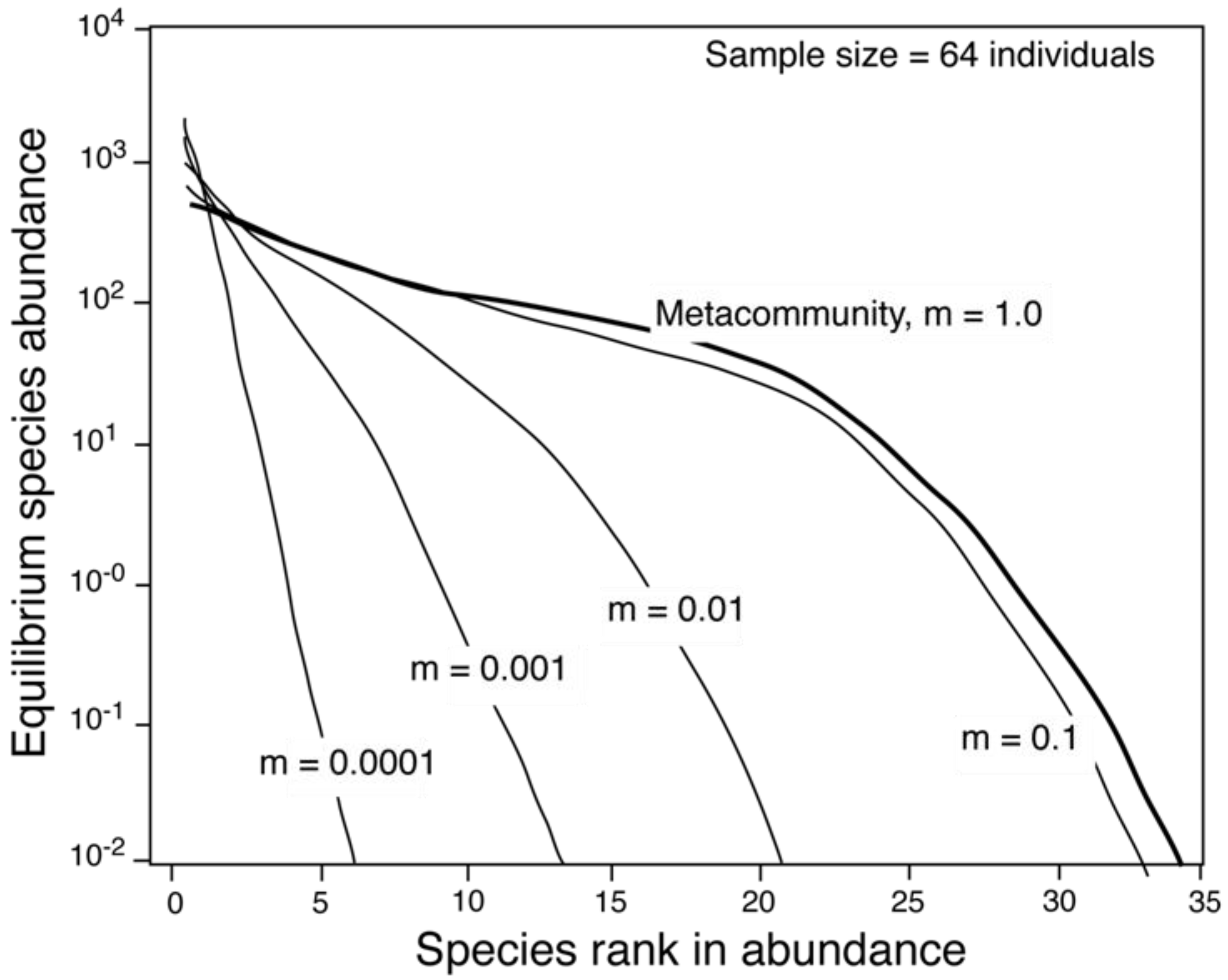
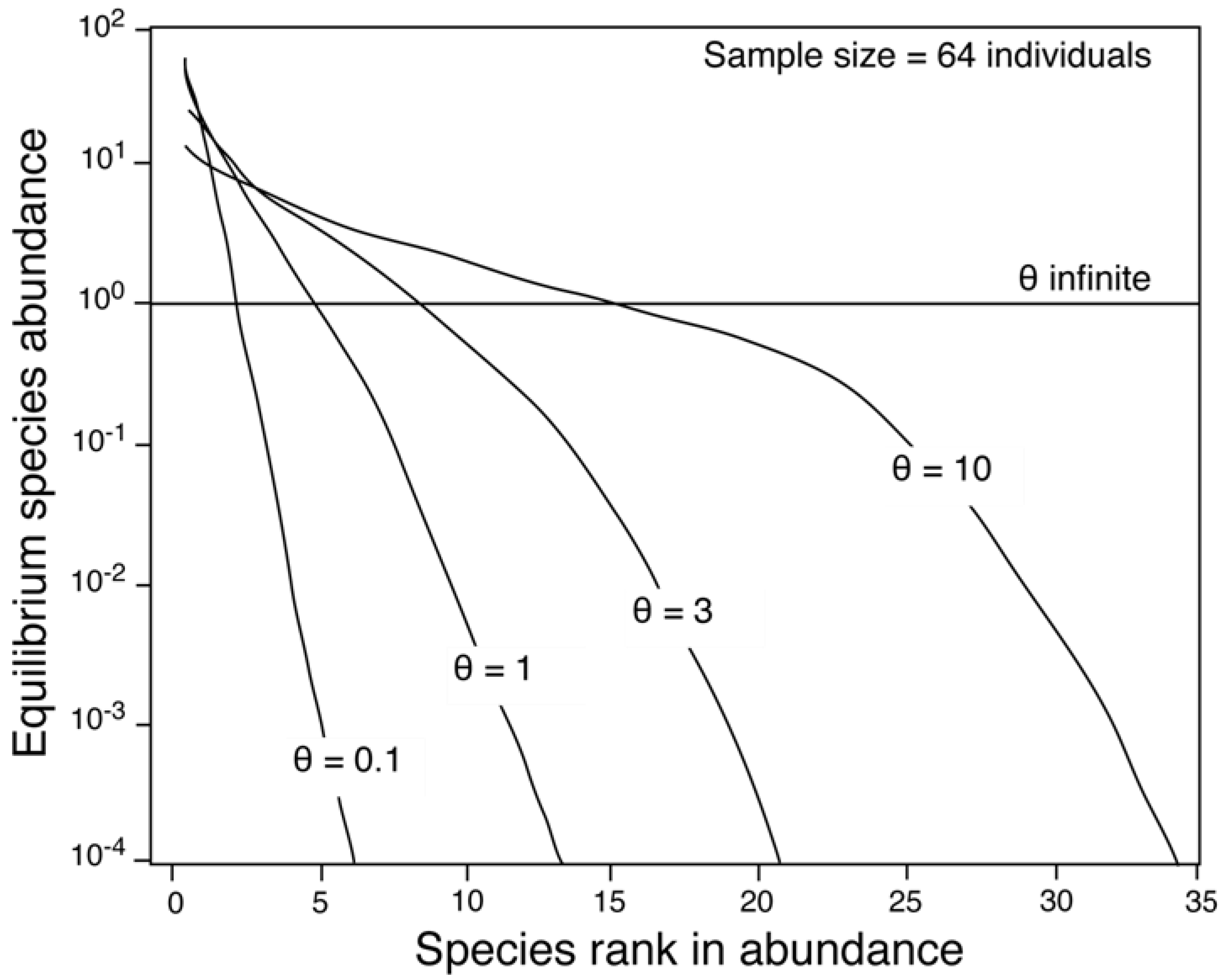
2.1. The Parameters θ and m

An important aspect of neutral theory is the fundamental biodiversity number θ, a dimensionless number that, along with the dispersal coefficient (m) governs the shape of a community’s relative abundance distribution [1]. As a reflection of species richness (diversity) and the similarity of species’ relative abundances (evenness), θ controls the length and slope of the relative abundance distribution of a community [1] (Figure 1). An increase in θ results in an increase in diversity and a decrease in monodominance as space in the community becomes occupied by more species with similar abundances [1]. The relative abundance distribution increases in length and decreases in slope until θ approaches its theoretical limit of infinity, at which point, the shape of the distribution approaches a horizontal line, and all species within the community have an abundance of one [1].
Figure 1. The effect of the fundamental biodiversity number, θ, on relative abundance distributions. Communities with a larger θ are more diverse and have greater evenness. Modified from Hubbell [1].
Diversity 05 00240 g001
The dispersal coefficient (m) is the probability that a death in the local community will be replaced by an immigrant from outside the local community but within the metacommunity [1].A metacommunity is a closed system; species can migrate between local communities within a metacommunity but not into or out of the metacommunity itself. As a result, m is a measure of dispersal limitation within the metacommunity. It also indicates patchiness within a metacommunity and reflects the amount of similarity between local and metacommunity abundance structures. A local community with an m close to one experiences less dispersal limitation and will have a relative abundance distribution that is more similar to the metacommunity than a local community with an m close to zero [1]. Since most local communities experience some degree of dispersal limitation, and because species that are rare in the metacommunity have a lower probability of dispersing to a local community, the relative abundance distribution of a local community will be shorter and steeper than that of the metacommunity [1] (Figure 2).
Figure 2. The effect of the dispersal coefficient, m, on the relative abundance distribution of a local community compared to that of the metacommunity. As m decreases, local communities (thin lines) differ increasingly from the metacommunity (bold line). Modified from Hubbell [1].
Diversity 05 00240 g002

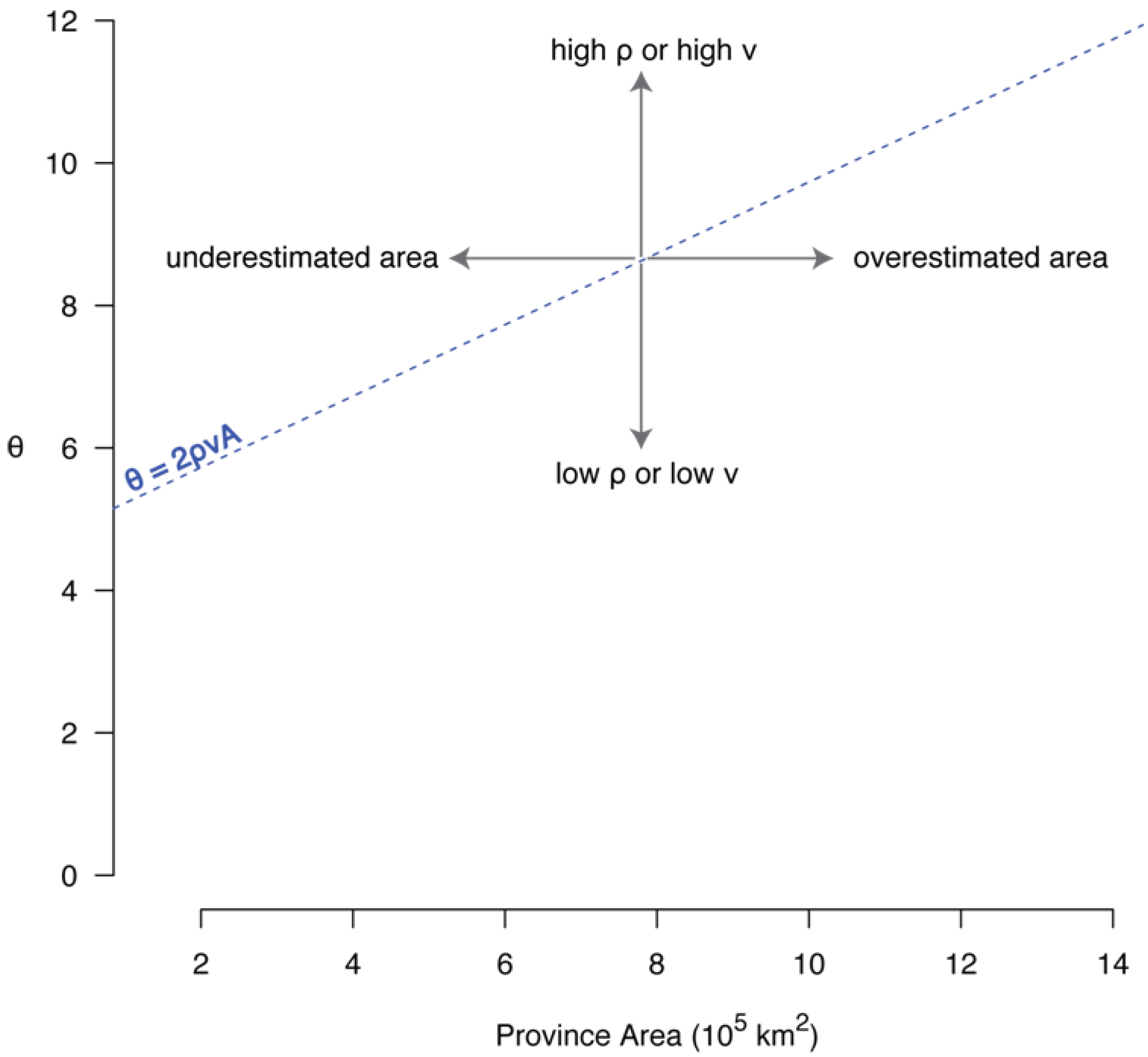
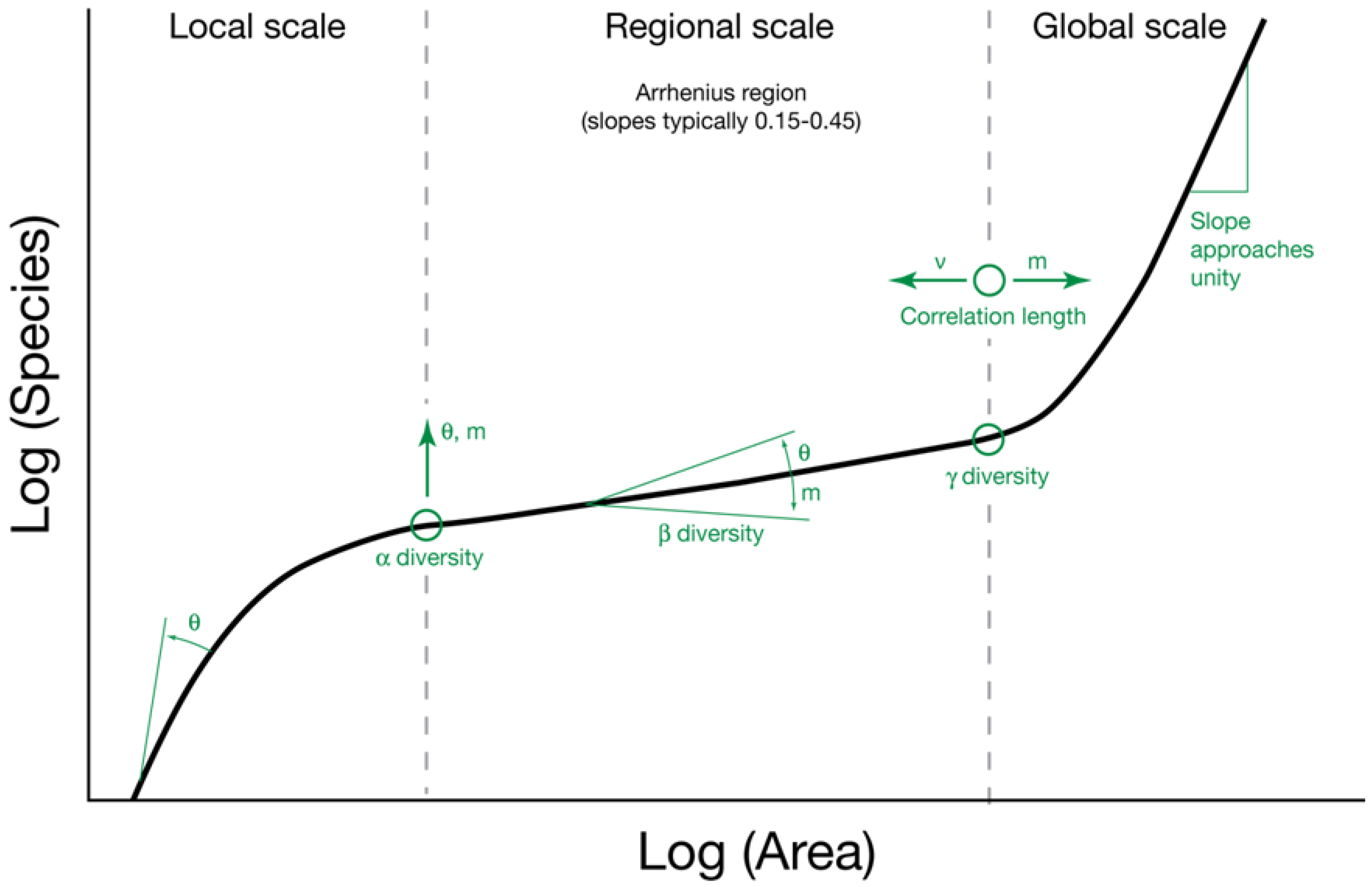
2.2. The Relationship between θ and Area

Hubbell derived θ from modeling the random walk of a dispersal-assembled community with a metacommunity size (Jm) and per-individual speciation rate (ν) [1]. From these two variables, Hubbell identified a constant parameter, 2Jmν, and called it θ [1]. Although this constant mathematically describes θ, it cannot be used to easily calculate θ because Jm is a very large number, ν is a very small probability, and both are nearly impossible to determine in practical applications [1]. In practice, likelihood methods are used to fit θ to an observed relative abundance distribution of species within a community.
Since neutral theory assumes that the space a community occupies is biologically saturated, the size of the metacommunity (Jm) is equal to the total area occupied by the metacommunity (Am), and the mean density of individuals in that area (ρ) [1]:
Diversity 05 00240 i001
This equation links the biodiversity of a metacommunity to the area occupied by the metacommunity, equivalent to a biogeographic province [1]. This linear relationship between diversity and province area is testable because θ can be estimated from census data, and the area of provinces can be measured from maps.

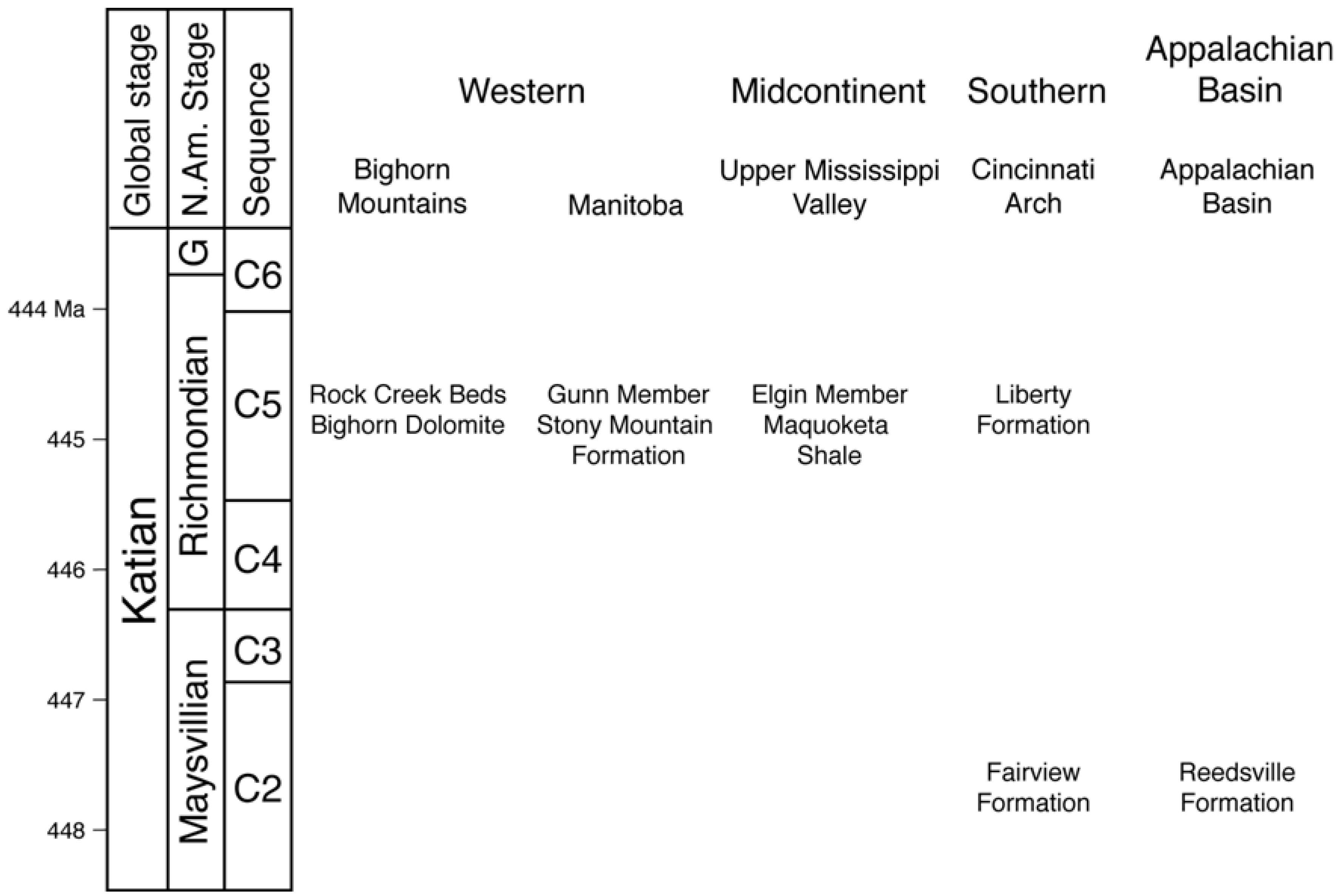
3. The Late Ordovician of Laurentia

In the Late Ordovician (443–458 Ma), Laurentia, the core of the continental landmass that is now North America, straddled the equator and lied entirely within tropical latitudes [11]. A shallow tropical epicontinental sea, similar to the modern day carbonate platform in the Bahamas, covered most of what is now the central United States and Canada. The southeastern margin of the continent was the site of the Taconic orogeny, which created a deeper water foreland basin in the area near the modern Appalachian Mountains [12].
Bathymetric differences across the Laurentian sea coupled with its vastness created oceanographically distinct geochemical regions [2,3,4]. Since these regions correspond to known faunal provinces, e.g., [13,14,15,16], they can be treated as separate metacommunities, or biogeographic provinces: the Appalachian Basin, Southern, Midcontinent, and Western provinces (Figure 3).
Figure 3. Late Ordovician paleogeography of Laurentia, showing the shallow seaway (blue), land (brown), and the location of four biogeographic provinces (provinces adapted from both [2] and [3], paleogeographic reconstruction from [17]). This study considers the area of only the deep subtidal facies, which for the Western Province is much smaller than total province area. The estimated extent of deep subtidal facies in the Western province is indicated by cross-hatching. Points represent sampling locations for the six data sets collected (BH: Bighorn Mountains, M: Manitoba, UMV: Upper Mississippi Valley, CA: Cincinnati Arch, AB: Appalachian Basin).
Diversity 05 00240 g003

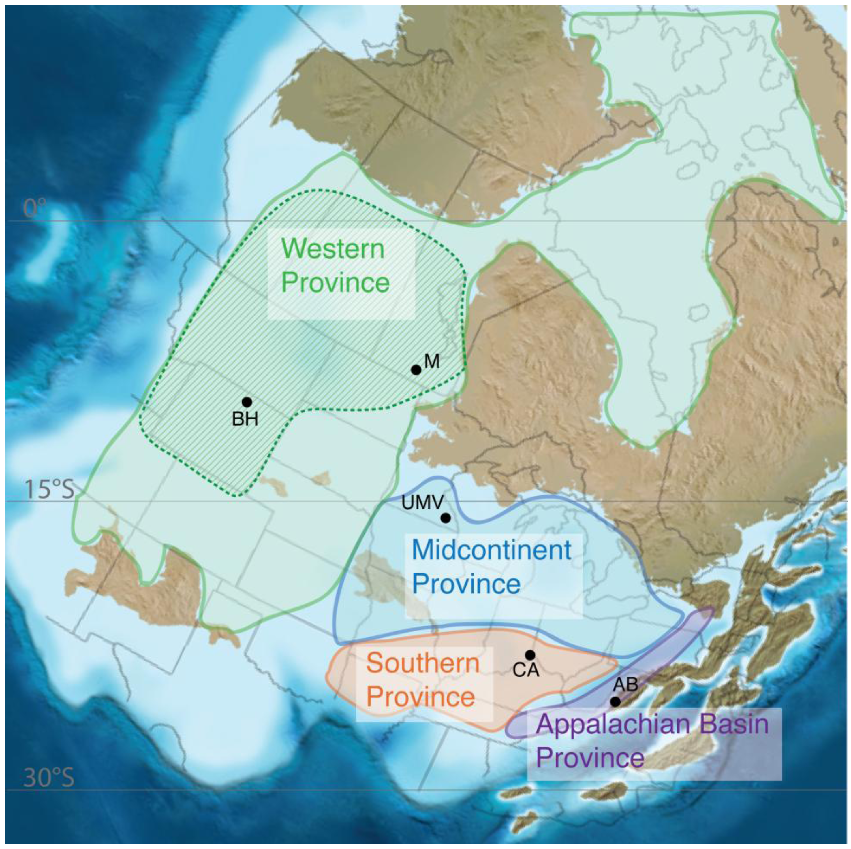
3.1. Geochemical Provinces

The Appalachian Basin, Southern, and Midcontinent provinces were defined primarily on differences in the εNd isotopic composition of conodonts (small phosphatic teeth of primitive fish) and the δ13C isotopic composition of limestone [2]. The εNd isotopic signature of conodonts reflects the crustal age of the continental landmass that serves as the primary source of sediment to a water mass, and it can vary greatly between regions [18]. The δ13C isotopic ratio of limestone varies only slightly in response to variations in biological productivity and burial, but can vary across carbonate platforms, e.g., [19]. Holmden et al. [2] used differences in εNd and δ13C in the Late Ordovician to identify strata that record deposition within the Appalachian Basin, Southern, and Midcontinent regions. In addition, differences in δ13C isotope values among these regions has been linked to different rates of carbon cycling [4], further supporting the evidence for limited mixing between water masses and linking these geochemical distinctions to biological activity. That these regions had distinct isotopic compositions suggests the presence of barriers to biological migration, and thus, that these areas would have been distinct biogeographic provinces.

3.2. Biogeographic Studies Support These Regions as Provinces

Although no comprehensive studies of provinciality in the Late Ordovician seas of Laurentia have yet been conducted, studies on particular taxa indicate that the geochemically defined water masses of Holmden et al. [2] are reflected in faunal distributions. For example, the faunal distinctiveness of the Appalachian Basin Province has been recognized previously in multiple studies, including those of conodont [13,14,20], graptolite [21,22,23,24], ostracod [25], and shelly fossil [26] assemblages. Studies of solitary rugosan corals indicate a province stretching from northern Illinois southward to Missouri and southwestward to Oklahoma [27], corresponding to the Midcontinent Province of Holmden et al. [2]. Rugosan corals [28] and bryozoans [16] support the presence of a province encompassing the Nashville Dome of Tennessee and the Cincinnati Arch of Ohio, Indiana, and Kentucky, similar to the Southern Province of Holmden et al. [2]. Finally, the vast region of the western United States and Canada has long been recognized as a faunally cohesive region, based on bryozoans [16], nautiloids [29], rugosans [15], brachiopods [30,31,32], and a distinctive Thalassinoides ichnofacies [3,33].
The boundaries of these faunally defined provinces do not always coincide precisely with one another or with the geochemically defined water masses. Many of these discrepancies can be attributed to how provincial boundaries are drawn between sampling locations. Other differences in boundary placement likely reflect that boundaries between provinces may have been permeable to varying degrees, with some taxa more able extend to nearby regions than others. Any uncertainty in the geographic extent of provinces caused by these factors would weaken the species-area relationships examined here.

4. Methods

Faunal censuses were used to produce estimates of θ from each of the provinces, whose areas were measured to test for a positive relationship between θ and area.

4.1. Data Collection

To minimize variation over time, faunal samples were obtained from the C2 and C5 depositional sequences [34] (Figure 4). To minimize variation in faunal composition caused by water depth, e.g., [35,36], all samples were collected from the deep subtidal depositional environment, that is, between fair weather and storm wave base.
Six data sets were used in this study (Figure 4): three from existing data (C2 Cincinnati Arch, C5 Cincinnati Arch, Bighorn Mountains) and three from newly collected data (Appalachian Basin, Upper Mississippi Valley, Manitoba). The C2 and C5 Cincinnati Arch data sets were collected from the Fairview Formation (C2) and Liberty Formation (C5) in the Cincinnati, Ohio area [36]. The Bighorn Mountains data set was obtained from the Rock Creek Beds of the Bighorn Dolomite (C5) in Wyoming [37]. The Appalachian Basin data set was collected from the Reedsville Formation (C2) near Catawba and Newport, Virginia, and from Germany Valley, West Virginia. The Upper Mississippi Valley data set was assembled from the Elgin Member of the Maquoketa Formation (C5) in Fillmore County, Minnesota. The Manitoba data set was obtained from the Gunn Member of the Stony Mountain Formation (C5) just north of Winnipeg, Manitoba. Each regional data set contains multiple local samples, with new data sets containing 25–30 samples and older data sets having 40–100 samples. Locality descriptions for the new data sets are included in Appendix 1.
In most data sets, sampling occurred over multiple beds, with each faunal sample representing a single bed. Samples for the Manitoba data set, however, were obtained as individual rock slabs from a spoil pile in a quarry, and it is unclear to what extent these slabs represent multiple beds.
Figure 4. Strata and time intervals sampled. Six data sets (Bighorn Mountains, Manitoba, Upper Mississippi Valley, Cincinnati Arch, Appalachian Basin) were collected from the C2 and C5 depositional sequences [34] across all four provinces.
Diversity 05 00240 g004
Censuses of marine invertebrates were conducted by identifying and counting all individuals in each sample. Individuals were identified to species where possible. All taxa were counted using whole-faunal counts with a minimum number of individuals approach [35]. This method calculates species abundance for brachiopods and bivalves as the total number of articulated valves, plus the greater of right or left disarticulated valves, plus one-half the number of indeterminate valves [35]. Bryozoans were identified to genus when possible, but mostly by morphological form and counted in 1 cm lengths to standardize for biovolume [35]. Colonial corals were also counted in 1 cm lengths, but were identified to genus. Solitary rugose corals and gastropods were identified to genus and counted as a single individual. Trilobites were counted only when identifiable, such as for pygidia and cranidia. Crinoids were noted if present but not counted since it is not possible to generate a number of individuals from columnals.
Prior to analysis, all data sets were culled to include only low-tier primary consumers to meet the neutral theory’s requirement of a single trophic level [1] (Table 1), with trophic level determined from the Paleobiology Database [38]. Primary consumers were selected for analysis because of their high abundance and recognizability in Ordovician samples. Focusing on only low-tier organisms, that is, those that live close to the sediment water interface, minimized any difference in nutrient access that height in the water column could provide to an organism.
Table 1. List of taxa included and excluded in the study.
Taxa IncludedTaxa Excluded
detritivore gastropods (ex: Liospira)carnivorous gastropods (ex: Subulites)
detritivore trilobites (ex: Isotelus)carnivorous trilobites (ex: Ceraurinus)
all brachiopodsall nautiloids
all coralsall crinoids
all bryozoansall algae
all bivalves
Samples with fewer than 24 individuals were removed from the data sets to ensure that each sample accurately represented the overall community and to increase statistical power, e.g., [35].

4.2. Data Analysis

4.2.1. Relative Abundance Distributions

Two types of relative abundance distributions were calculated in R [39]. A distribution that reflects the abundance distribution for local communities was calculated from the mean abundance of each species across all samples within a data set. A distribution that reflects the abundance distribution of the metacommunity was calculated from the total abundance of each species in the whole data set. Comparing the local and metacommunity relative abundances in this manner illustrates how well diversity in an average sample reflects the diversity in the province [1].

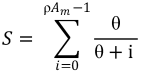
4.2.2. Estimation of θ

Hubbell’s θ was estimated using Etienne’s 2007 [40] and 2009 [41] likelihood methods. These methods calculate θ for the metacommunity and m for the local communities by using a numerical optimization over a range of possible values to determine the combination of θ and m with the maximum likelihood. These likelihood methods were performed in PARI/GP [42].
The major difference between the two methods is that the 2007 method assumes that all local communities experience the same amount of dispersal limitation, and it estimates a single m value for all local communities within the metacommunity [40]. The 2009 method allows each local community to experience a different amount of dispersal limitation, and it produces a different estimate of m for each local community [41]. Consequently, the 2007 method searches over a 2-dimensional parameter space, runs in a few minutes, and produces a visualizable likelihood surface. The 2009 method searches over an n+1 dimensional space where n is the number of samples, runs for a few hours for smaller data sets to several months for larger data sets, and does not result in a visualizable likelihood surface.

4.2.3. Estimation of Area

Province area was calculated using ArcGIS [43]. The calculate geometries tool was used to measure the area of polygons of the estimated size and shape of each province on an equal-area map of North America. The approximate geographic location and extent of the provinces were determined using published maps and data from previous studies [2,3] and personal knowledge of Ordovician faunal distributions.
Although the deep subtidal environment was broadly distributed across large portions of the Midcontinent, Southern, and Appalachian Basin provinces, it is confined to a relatively small portion of the Western province. Well log data [44,45,46,47] were used to identify known subsurface locations of the deep subtidal Gunn Member and correlative strata, such as the Rock Creek beds of Wyoming [44]. Additional studies, e.g., [48] of locations at which the deep subtidal are absent and of the location of anhydrites associated with the center of the Williston Basin, e.g., [47] were used to constrain the estimated extent of the deep subtidal facies to the north, south, and east (Figure 3). Because of widespread erosion of Ordovician rocks during the Devonian [46], the western extent of the deep subtidal facies could not be constrained more than the estimated western boundary of the province.

5. Results

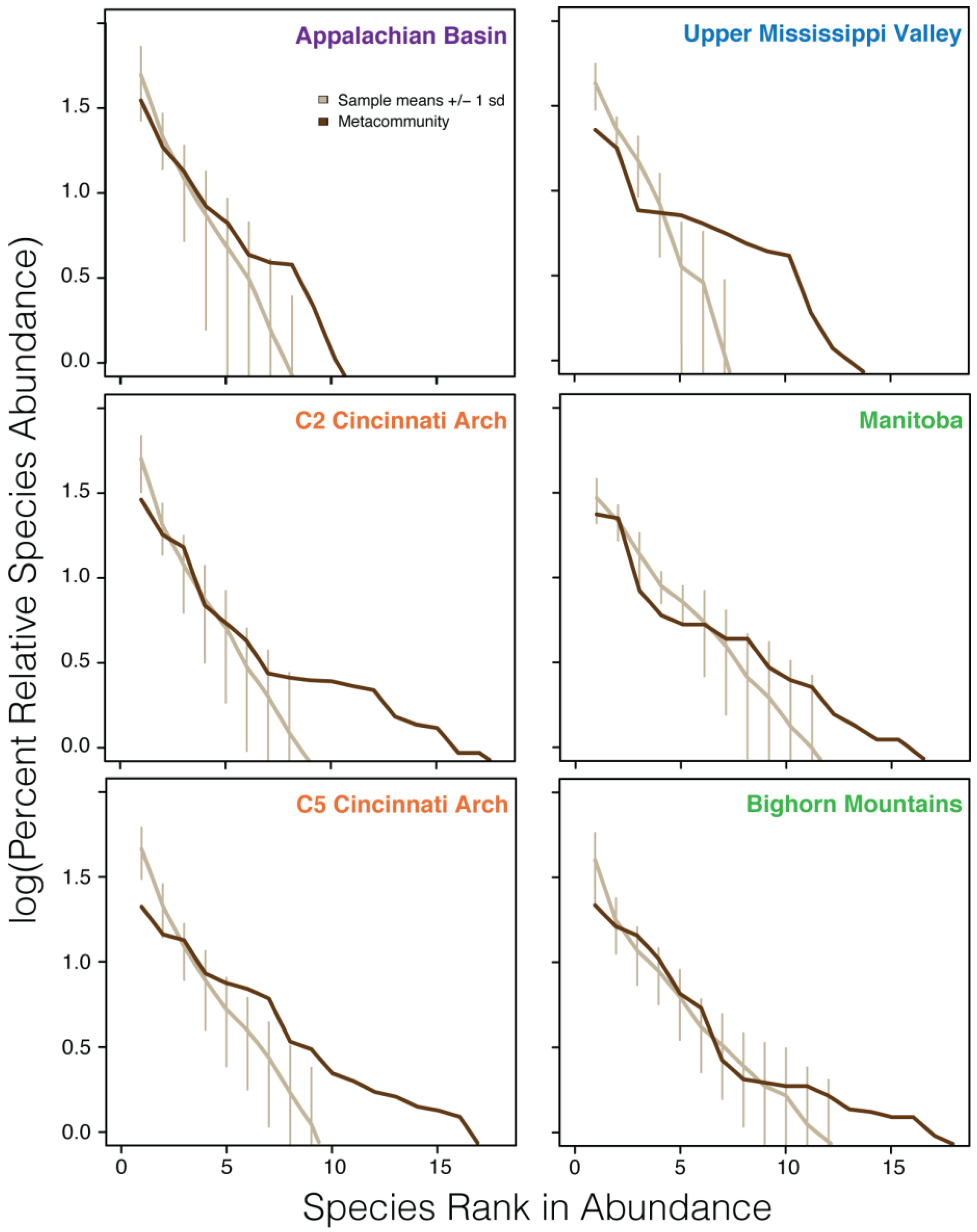
5.1. Relative Abundance Distributions

All data sets used in this study are dominated by a few abundant species (Figure 5). The metacommunity abundance distribution for the Appalachian Basin data set is the steepest and has the fewest species, and the distribution for the Bighorn Mountains has the lowest slope and the greatest species richness. In general, data sets with a larger total number of species in the metacommunity (e.g., Cincinnati Arch and Bighorn Mountains) display a long tail of rare species, which mitigates the abundance value of the most dominant species (Table 2).
The long tail of rare species likely reflects the large number of samples because increased sampling results in the “unveiling” of more singleton species [49]. However, as long as the data set contains local samples that when combined are representative of the metacommunity [1], the effect of sample size on the estimate of θ should be minimal.
Figure 5. Relative abundance distributions for each data set, showing the comparison between total metacommunity abundances (dark brown line) and means and standard deviations of local community abundances (tan line).
Diversity 05 00240 g005
In all data sets except the Upper Mississippi Valley, the means of local community abundances are a good approximation of the metacommunity abundances for taxa that are neither the rarest nor the most abundant. For the Upper Mississippi Valley data set, the local community abundance distribution poorly approximates the metacommunity abundance distribution, and most local samples are much less diverse than the metacommunity. For all data sets, the most abundant taxa in the metacommunity tend to be slightly overrepresented in the local communities, whereas rare taxa and singletons in the metacommunity are often absent from individual local collections. Consequently, total species richness and evenness in local communities is less than that of the metacommunity (Table 2).
Table 2. Comparison between metacommunity and local community species richness, including sample sizes for each data set.
Data setNumber of samplesMetacommunity species richnessMean local community species richness
Appalachian Basin23207
C2 Cincinnati Arch63318
C5 Cincinnati Arch99439
Upper Mississippi Valley9217
Manitoba122211
Bighorn Mountains394911

5.2. Estimation of θ and Area

Estimates of θ (Table 3) fall within a range consistent with values estimated by Hubbell for modern benthic marine invertebrate communities [1]. Previously reported values of θ range from 3 for a low diversity boreal community to 20 for a highly diverse tropical community. Values of θ estimated in this study are reasonable given this range, but are somewhat low given that the epicontinental sea of Laurentia was positioned entirely within tropical latitudes.
The Appalachian Basin data set has both the lowest θ and area, and the Bighorn Mountains data set has the largest θ and area (Table 3). Manitoba has an unusually low θ given the large area of the Western Province. In addition, although both the Manitoba and Bighorn Mountains data sets represent the Western province, their estimated values of θ differ.
Table 3. Results from the estimation of θ and area. The multi-dimensional 2009 method was not able to calculate θ for some data sets due to sample size.
Data setθ 2007 method [40]θ 2009 method [41]Province area (km2)
Appalachian Basin5.225.431.35 x 105
C2 Cincinnati Arch6.32not calculated4.81 x 105
C5 Cincinnati Arch8.49not calculated4.81 x 105
Upper Mississippi Valley8.798.689.27 x 105
Manitoba5.47not calculated13.9 x 105
Bighorn Mountains11.910.013.9 x 105
Although θ was calculated using both Etienne methods [40,41] only the results from the 2007 method [40] are used for subsequent analysis. The 2009 method [41] successfully calculated a θ for only three of the data sets (Appalachian Basin, Upper Mississippi Valley, and Bighorn Mountains). For the other three data sets, the likelihood estimation either did not finish running after three months because the data sets were too large (C2 Cincinnati and C5 Cincinnati) or produced an error (Manitoba). For the three data sets for which the multi-dimensional 2009 method [41] was successful, the estimated θ is similar to that of the 2-dimensional 2007 method [40], suggesting that the results of the 2007 method are reliable.

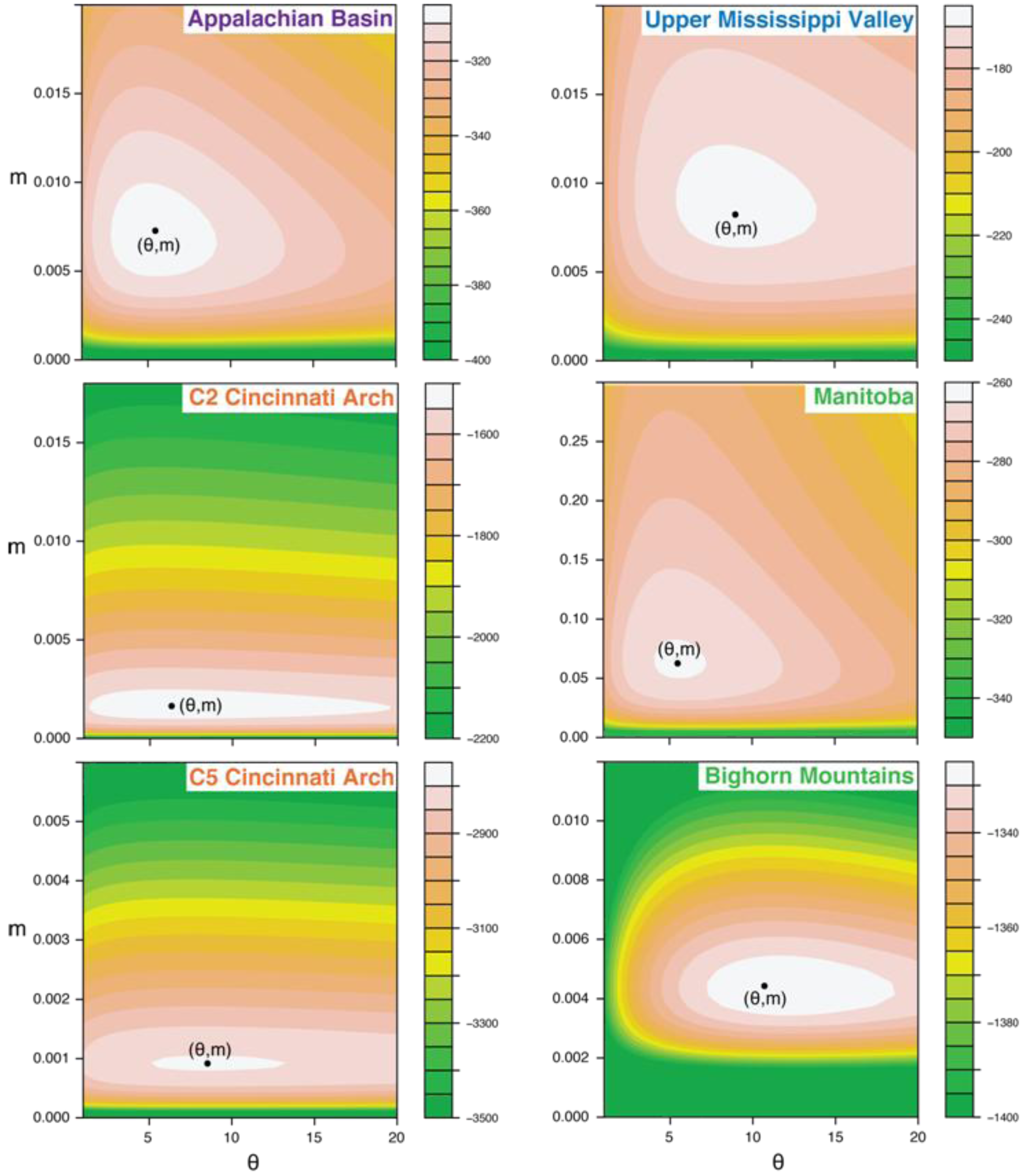
5.3. Likelihood Surfaces

Likelihood surfaces illustrate the uncertainty in the estimates of θ and m (Figure 6). The confidence region is smallest for the three existing data sets (C2 Cincinnati, C5 Cincinnati, Bighorn Mountains), reflecting the greater number of samples in these data sets. For all data sets, m is tightly constrained, whereas the estimate of θ has more uncertainty. The estimated values of m are less than 0.01 for all data sets except Manitoba, which has a slightly higher m (0.064). These values indicate strong dispersal limitation and little to no migration from the metacommunity into local communities [1]. Such large dispersal limitation is unexpected for marine organisms, which disperse by releasing larvae into the water column.
Figure 6. Likelihood contour surfaces for each data set. Maximum likelihood estimates from the 2007 method [40] are indicated with black dots.
Diversity 05 00240 g006

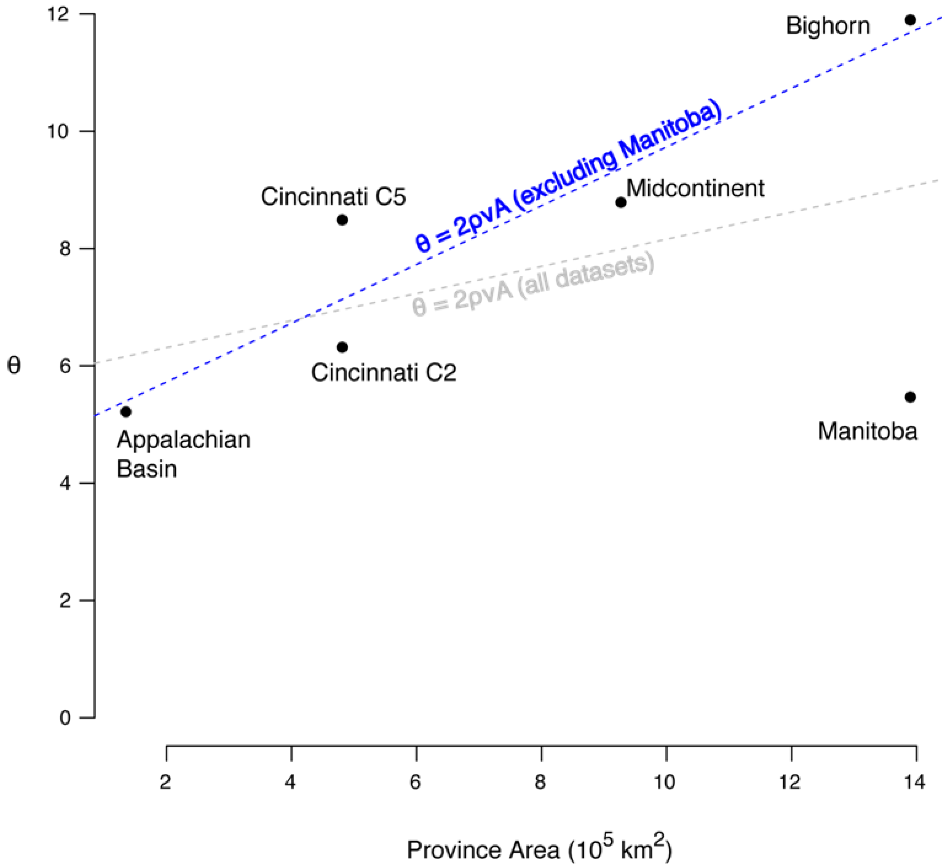
5.4. Correlation between θ and Area

Province area and θ are weakly and positively correlated, although below statistical significance (R2 = 0.03, p = 0.34). The trend line of the correlation between θ and area is positive (Figure 7) with a slope of 2ρν. If the Manitoba data set is treated as an outlier and removed from analysis (see below), the correlation strengthens and becomes statistically significant (R2 = 0.85, p = 0.02).
Figure 7. Correlation between θ and province area. The dotted lines are trend lines and have a slope of 2ρν. The grey dotted line includes all data sets, and the blue dotted line excludes the Manitoba data set.
Diversity 05 00240 g007

6. Discussion

6.1. The Correlation between θ and Area

The weakly positive correlation between θ and area indicates that province area exerts some control on regional biodiversity. When the Manitoba data set is excluded, the correlation is substantially stronger suggesting that province area is a significant driver of regional biodiversity.
The collecting conditions in Manitoba differ from those of all other locations, which might explain the unusual estimates of θ and m for the Manitoba data set and would support treating it as an outlier. At all other sampling locations, it was possible to collect samples that were clearly from different beds. Due to limited exposure in Manitoba, samples were available only from a spoil pile in a quarry. Because of this, these samples may represent many fewer beds than the total number of samples would suggest. If all of the Manitoba samples were collected from the same bed, they would represent repeated sampling of a single local community as opposed to multiple local samples of the full metacommunity. Not sampling the full metacommunity would result in an artificially larger m and smaller θ. The Manitoba data set does have a lower θ than expected and it is the only data set to have an m greater than 0.01.
The slope of the trend line reflects a constant relationship between the density of organisms per unit area within the habitat (ρ) and the per-individual probability of speciation (ν), but it is likely that these factors vary among the metacommunities substantially enough to affect biodiversity. A stronger than expected influence of one or both of these variables would introduce scatter in the θ-area correlation and account for some of the deviation from the expected linear relationship. A large ρ or ν would result in a larger θ for a data set and cause it to plot above the trend line, while a small ρ or ν would result in a smaller θ, causing the data set to plot below the trend line (Figure 8).
Figure 8. Causes of scatter around the trend line between θ and province area.
Diversity 05 00240 g008
Differences in habitat density could easily be caused by differences in food supply or substrate. For example, a region with high productivity and more suspended organic matter could support a higher density of suspension feeders than one with lower productivity [50]. This could explain why the Bighorn Mountains and Cincinnati C5 data sets, which both contain a tropical fauna, plot above the trend line while the Appalachian Basin and Cincinnati C2 data sets, which contain a cooler water fauna, plot below the line [51].
A latitudinal temperature gradient between the cooler water Appalachian Basin fauna and the equatorial Western fauna could cause variation in speciation rate, with higher speciation rates occurring in the warmer water regions, e.g., [52,53,54]. However, since Hubbell’s ν is a per-individual speciation rate as opposed to a per-species speciation rate as is generally measured, it is difficult to test whether this gradient is indeed a source of variation in θ.
An additional explanation for scatter in the data is underestimation or overestimation of province area. Overestimates of area shift points to the right of the trend line and underestimates of area shift points to the left (Figure 8). Although lithological, faunal, and geochemical data were all used to provide evidence for province boundaries, there is still a degree of uncertainty in province area mainly because burial of strata in the subsurface and erosion of strata limit the accessibility of Ordovician rocks. This could artificially weaken or strengthen the correlation between θ and area and be especially problematic for provinces in which there is a large difference between the area of the deep subtidal facies and the total area of the province.
Because sampling was limited to deep subtidal strata, uncertainty in the extent to which this habitat spanned the province could add to the uncertainty in area. For the Western province, the deep subtidal habitat is demonstrably limited to only a portion of the province, and it is this smaller area that was used in the analysis. The deep subtidal facies is likely also limited, but to a lesser extent, for the Midcontinent province, but is much more difficult to estimate. An overestimation of the deep subtidal habitat area could explain why the Midcontinent province plots to the right of the trend line. It is unlikely that possible error in the area estimate has a significant effect on the Southern and Appalachian Basin provinces because both regions have widespread and well-constrained regions of deep subtidal strata.
Additionally, the observed scatter in the relationship between θ and province area could reflect non-neutral community dynamics. If interspecific competition has a significant effect on the abundance structure of the community, the assumption of neutrality would be invalid. Competition within a community could increase under environmental conditions that limit resource availability.

6.2. The Species-Area Relationship and θ

Hubbell’s θ is significant for diversity studies because it links diversity across spatial scales. From the local to the global scale, the species-area relationship is triphasic, e.g, [55,56,57,58]. Hubbell [1] argued that θ and m are important controls on the shape of the triphasic curve at each spatial scale (Figure 9). At the local scale, species richness increases curvilinearly with area, reflecting a sampling curve in which new species are initially encountered rapidly but then more slowly as area increases [1]. At the regional scale, species richness increases log-linearly as the addition of new local communities increases the potential to add new species with each increase in area [1]. At the global scale, diversity initially increases exponentially but then the slope approaches unity as metacommunities with entirely different species compositions are encountered [1].
At the local scale, θ and m have a combined effect on the species-area relationship [1]. The slope of the initial part of the curve steepens with θ, such that a larger θ corresponds to a more rapid rise in the number of species as a local community is sampled. Total diversity of the local community, or alpha diversity, which occurs at the point on the curve at which the relationship switches from local to regional dynamics, is affected by both θ and m. Larger values of θ and m result in a greater alpha diversity, while lower values of θ and m will lower alpha diversity.
At the regional scale, θ and m have inverse effects on the species area relationship [1]. A larger θ will increase both the slope of the log-linear relationship (beta diversity) and the province diversity (gamma diversity). A larger m has the opposite effect, decreasing beta and gamma diversity. Total gamma diversity also corresponds to the point at which the species-area relationship shifts from regional to global dynamics, called the correlation length. This point is affected by m and ν, such that a larger ν causes a smaller correlation length and a larger m produces a larger correlation length.
Figure 9. The triphasic relationship between species and area. The relationship between species richness and area varies across spatial scales and is controlled by θ and m. The effects of θ and m on the shape of the curve and local (alpha), regional (beta), and global (gamma) diversity are indicated by arrows. Based on Hubbell [1].
Diversity 05 00240 g009
At the global scale, the effects of θ and m on the species-area relationship are uncertain. At this scale, species richness and area increase as multiple provinces are combined to accumulate global diversity [1]. The amount of diversity added with each province depends on the degree to which provinces differ from each other. Total global diversity increases with the number of provinces and their dissimilarity from each other.
Since θ and m drive alpha, beta, and gamma diversity, diversity at local and provincial scales are linked, such that processes affecting diversity and abundance in the local community have inherent implications for diversity and abundance in the metacommunity. This link between local communities and the metacommunity reflects a continuous landscape over which local-scale diversity patterns increasingly resemble that of the metacommunity at larger spatial scales [59].
The manner in which diversity increases between these two spatial scales is important to describing how diversity is assembled globally and may help to understand the origin of changes in Phanerozoic diversity [60,61,62,63]. Since the θ-area relationship exists in the Late Ordovician, and likely throughout the fossil record (though future work will need to test this), it should be possible to predict species richness of a given province from the area and habitat density of a province and an estimate of θ, as suggested by Hubbell [1]:
Diversity 05 00240 i002
Province area can be estimated from paleogeographic maps and θ can be estimated from a collection of local samples, so, given a method to estimate habitat density, this equation could be used to estimate species richness for any province in the Phanerozoic.

7. Conclusions

(1) The fundamental biodiversity number (θ) and province area are positively correlated in Late Ordovician marine communities of Laurentia, as predicted by Hubbell’s [1] neutral theory. The strength of the correlation is likely affected by uncertainties in the estimates of province area and variations in the habitat density per unit area (ρ) and the per-individual speciation rate (ν).
(2) Hubbell’s θ and m link local and province-scale diversity across the triphasic species-area relationship [1,59]. Because of these linkages, local community diversity has implications for the diversity of provinces. This linkage could be exploited to understand causes for changes in Phanerozoic diversity.

Acknowledgments

We thank Jon Primm and Ally Platsky for assisting in fieldwork, Mark Patzkowsky for collecting faunal data from the Cincinnati Arch and Bighorn Mountains, Ed Dobrzanski and Graham Young at The Manitoba Museum for providing information about Manitoba geology, Warren Netherton of Mystery Cave State Park for providing information about Minnesota geology, and two anonymous reviewers for providing comments and suggestions. We also thank the Mariash Construction Quarry and Milestone Materials for allowing outcrop access. This research was supported by the Geological Society of America, the Paleontological Society, the Theodore Roosevelt Memorial Fund, Sigma Xi Grants-in-Aid of Research, the Miriam Watts-Wheeler Fund, and the National Science Foundation (NSF EAR-0948895).

Conflict of Interest

The authors declare no conflict of interest.

References

  1. Hubbell, S.P. The Unified Neutral Theory of Biogeography; Princeton University Press: Princeton, NJ, USA, 2001; p. 375. [Google Scholar]
  2. Holmden, C.; Creaser, R.A.; Muehlenbachs, K.; Leslie, S.A.; Bergström, S.M. Isotopic evidence for geochemical decoupling between ancient epeiric seas and bordering oceans: implications for secular curves. Geology 1998, 26, 567–570. [Google Scholar]
  3. Jin, J.; Harper, D.A.T.; Rasmussen, J.A.; Sheehan, P.M. Late Ordovician massive-bedded Thalassinoides ichnofacies along the paleoequator of Laurentia. Palaeogeogr. Palaeocl. 2012, 367–368, 73–88. [Google Scholar]
  4. Panchuk, K.M.; Holmden, C.E.; Leslie, S.A. Local controls on carbon cycling in the Ordovician midcontinent region of North America, with implications for carbon isotope secular curves. J. Sediment. Res. 2006, 76, 200–211. [Google Scholar] [CrossRef]
  5. Alonso, D.; Etienne, R.S.; McKane, A.J. The merits of neutral theory. Trends Ecol. Evol. 2006, 21, 451–457. [Google Scholar] [CrossRef]
  6. Purves, D.W.; Turnbull, L.A. Different but not equal: the implausible assumption at the heart of neutral theory. J. Anim. Ecol. 2010, 79, 1215–1225. [Google Scholar] [CrossRef] [Green Version]
  7. Rosindell, J.; Hubbell, S.P.; Etienne, R.S. The unified neutral theory of biodiversity and biogeography at age ten. Trends Ecol. Evol. 2010, 26, 340–348. [Google Scholar] [CrossRef]
  8. Hubbell, S.P. The neutral theory of biodiversity and biogeography and Stephen Jay Gould. Paleobiology 2005, 31, 122–132. [Google Scholar] [CrossRef]
  9. Olszewski, T.D.; Erwin, D.H. Dynamic response of Permian brachiopod communities to long-term environmental change. Nature 2004, 428, 738–741. [Google Scholar] [CrossRef]
  10. Tomašových, A.; Kidwell, S.M. Predicting the effects of increasing temporal scale on species composition, diversity, and rank abundance distributions. Paleobiology 2010, 36, 672–695. [Google Scholar] [CrossRef]
  11. Scotese, C.R.; McKerrow, W.S. Ordovician plate tectonic reconstructions. Geol. S. Can. Paper 1991, 90, 271–282. [Google Scholar]
  12. Beaumont, C.; Quinlan, G.; Hamilton, J. Orogeny and stratigraphy: Numerical models of the Paleozoic in the eastern interior of North America. Tectonics 1988, 7, 389–416. [Google Scholar] [CrossRef]
  13. Sweet, W.C.; Bergström, S.M. Provincialism exhibited by Ordovician conodont faunas. SEPM Spec. P. 1974, 21, 189–202. [Google Scholar]
  14. Barnes, C.R.; Fåhræus, L.E. Provinces, communities, and the proposed nektobenthic habit of Ordovician conodontophorids. Lethaia 1975, 8, 133–149. [Google Scholar] [CrossRef]
  15. Elias, R.J. Solitary rugose corals of the Stony Mountain Formation, Southern Manitoba, and its equivalents. J. Paleontol. 1983, 57, 924–956. [Google Scholar]
  16. Antsey, R.L. Bryozoan provinces and patterns of generic evolution and extinction in the Late Ordovician of North America. Lethaia 1986, 19, 33–51. [Google Scholar] [CrossRef]
  17. Blakey, R. Global Paleogeography. Available online: http://jan.ucc.nau.edu/rcb7/globaltext2.html/ (accessed on 18 April 2012).
  18. Piepgras, D.J.; Wasserburg, G.J. Neodymium isotopic variations in seawater. Earth Planet. Sc. Lett. 1980, 50, 128–138. [Google Scholar] [CrossRef]
  19. Patterson, W.P.; Walter, L.M. Depletion of 13C in seawater ΣCO2 on modern carbonate platforms: significance for the carbon isotopic record of carbonates. Geology 1994, 22, 885–888. [Google Scholar] [CrossRef]
  20. Bergström, S.M. Biogeography, evolutionary relationships, and biostratigraphic significance of Ordovician platform conodonts. Foss. Strata 1983, 15, 35–58. [Google Scholar]
  21. Riva, J. A revision of some Ordovician graptolites of eastern North America. Palaeontology 1974, 17, 1–40. [Google Scholar]
  22. Bergström, S.M.; Mitchell, C.E. The graptolite correlation of the North American Upper Ordovician standard. Lethaia 1986, 19, 247–266. [Google Scholar] [CrossRef]
  23. Berry, W.B.N. Review of late Middle Ordovician graptolites in eastern New York and Pennsylvania. Am. J. Sci. 1970, 269, 304–313. [Google Scholar] [CrossRef]
  24. Goldman, D.; Bergström, S.M.; Mitchell, C.E. Revision of the Zone 13 graptolite biostratigraphy in the Marathon, Texas, standard succession and its bearing on Upper Ordovician graptolite biostratigraphy. Lethaia 1995, 28, 115–128. [Google Scholar] [CrossRef]
  25. Mohibullah, M.; Williams, M.; Vandenbroucke, T.R.A.; Sabbe, K.; Zalasiewicz, J.A. Marine ostracod provinciality in the Late Ordovician of palaeocontinental Laurentia and its environmental and geographical expression. PLOS one 2012, 7, e41682. [Google Scholar]
  26. Bretsky, P.W. Central Appalachian Late Ordovician communities. Geol. Soc. Am. Bull. 1969, 80, 193–212. [Google Scholar] [CrossRef]
  27. Elias, R.J.; Young, G.A. Coral diversity, ecology, and provincial structure during a time of crisis: the latest Ordovician to earliest Silurian Edgewood Province in Laurentia. Palaios 1998, 13, 98–112. [Google Scholar] [CrossRef]
  28. Elias, R.J. Latest Ordovician solitary rugose corals of eastern North America. Bull. Am. Paleontol. 1982, 81, 1–85. [Google Scholar]
  29. Flower, R.H. Ordovician cephalopods of the Cincinnati region, part 1. Bull. Am. Paleontol. 1946, 29, 1–656. [Google Scholar]
  30. Nelson, S.J. Arctic Ordovician fauna: an equatorial assemblage. J. Alberta Soc. Petr. Geol. 1959, 7, 45–47. [Google Scholar]
  31. Jin, J.; Zhan, R.B. Late Ordovician Articulate Brachiopods from the Red River and Stony Mountain Formations, Southern Manitoba; NRC Research Press: Ottawa, Canada, 2001; p. 117. [Google Scholar]
  32. Jin, J.; Caldwell, W.G.E.; Norford, B.S. Late Ordovician brachiopods Rafinesquina lata Whiteaves, 1896 and Kjaerina hartae n. sp. from southern Manitoba and the Hudson Bay lowlands. Can. J. Earth Sci. 1995, 32, 1255–1266. [Google Scholar] [CrossRef]
  33. Jin, J.; Harper, D.A.T.; Cocks, L.R.M.; McCausland, P.J.A.; Rasmussen, C.M.Ø.; Sheehan, P.M. Precisely locating the Ordovician equator in Laurentia. Geology 2013, 41, 107–110. [Google Scholar] [CrossRef]
  34. Holland, S.M.; Patzkowsky, M.E. Sequence stratigraphy and long-term paleoceanographic change in the Middle and Upper Ordovician of the eastern United States. Geol. Soc. Am. S. 1996, 306, 117–129. [Google Scholar]
  35. Holland, S.M.; Patzkowsky, M.E. Ecosystem structure and stability: Middle Upper Ordovician of central Kentucky, USA. Palaios 2004, 19, 316–331. [Google Scholar] [CrossRef]
  36. Holland, S.M.; Patzkowsky, M.E. Gradient ecology of a biotic invasion: biofacies of the type Cincinnatian Series (Upper Ordovician), Cincinnati, Ohio region, USA. Palaios 2007, 22, 392–407. [Google Scholar] [CrossRef]
  37. Holland, S.M.; Patzkowsky, M.E. Stratigraphic architecture of a tropical carbonate platform and its effect on the distribution of fossils: Ordovician Bighorn Dolomite, Wyoming, USA. Palaios 2009, 24, 303–317. [Google Scholar] [CrossRef]
  38. Paleobiology Database Home Page. Available online: http://paleodb.org/ (accessed on 29 September 2012).
  39. R Development Core Team. R: A Language and Environment for Statistical Computing; R Foundation for Statistical Computing: Vienna, Austria, 2011. ISBN 3-900051-07-0. Available online: http://www.R-project.org/ (accessed on 19 August 2011).
  40. Etienne, R.S. A neutral sampling formula for multiple samples and an ‘exact’ test of neutrality. Ecol. Lett. 2007, 10, 608–618. [Google Scholar] [CrossRef]
  41. Etienne, R.S. Maximum likelihood estimation of neutral model parameters for multiple samples with different degrees of dispersal limitation. J. Theor. Biol. 2009, 257, 510–514. [Google Scholar] [CrossRef]
  42. PARI/GP Home Page. Available online: http://pari.math.u-bordeaux.fr/ (accessed on 3 April 2012).
  43. ESRI, ArcGIS Desktop: Release 10, Environmental Systems Research Institute: Redlands, CA, USA, 2011.
  44. Holland, S.M.; Patzkowsky, M.E. Sequence architecture of the Bighorn Dolomite, Wyoming, USA: Transition to the Late Ordovician icehouse. J. Sediment. Res. 2012, 82, 599–615. [Google Scholar] [CrossRef]
  45. Lobdell, F.K. Arthrostylidae (Bryozoa: Cryptostomata) from the Gunn Member, Stony Mountain Formation (Upper Ordovician), North Dakota and Manitoba. N. Dak. Geol. Survey Misc. Series 1992, 76, 99–115. [Google Scholar]
  46. Richards, P.W.; Nieschmidt, C.L. The Bighorn Dolomite and Correlative Formations in Southern Montana and Northern Wyoming (Oil and Gas Investigations Map, OM-202) [Map]; U.S. Geological Survey: Reston, Virginia, VA, USA, 1961. [Google Scholar]
  47. Longman, M.W.; Fertal, T.G.; Glennie, J.S. Origin and geometry of Red River Dolomite reservoirs, western Williston Basin. AAPG Bull. 1983, 67, 744–771. [Google Scholar]
  48. Sweet, W.C. Harding and Fremont Formations, Colorado. AAPG Bull. 1954, 38, 284–305. [Google Scholar]
  49. Preston, F.W. The commonness and rarity of species. Ecology 1948, 29, 254–283. [Google Scholar] [CrossRef]
  50. Rex, M.A. Community structure in the deep-sea benthos. Annu. Rev. Ecol. Syst. 1981, 12, 331–353. [Google Scholar]
  51. Patzkowsky, M.E.; Holland, S.M. Extinction, invasion, and sequence stratigraphy: patterns of faunal change in the Middle and Upper Ordovician of the eastern United States. Geol. S. Am. S. 1996, 306, 131–142. [Google Scholar]
  52. Allen, A.P.; Gillooly, J.F.; Savage, V.M.; Brown, J.H. Kinetic effects of temperature on rates of genetic divergence and speciation. Proc. Natl. Acad. Sci. USA 2006, 103, 9130–9135. [Google Scholar]
  53. Jablonski, D.; Roy, K.; Valentine, J.W. Out of the tropics: evolutionary dynamics of the latitudinal diversity gradient. Science 2006, 314, 102–106. [Google Scholar] [CrossRef]
  54. Crame, J.A. Evolution of taxonomic diversity gradients in the marine realm: a comparison of Late Jurassic and Recent bivalve faunas. Paleobiology 2002, 28, 184–207. [Google Scholar] [CrossRef]
  55. Rosenzweig, M.L. Species Diversity in Space and Time; Cambridge University Press: Cambridge, UK, 1995; p. 436. [Google Scholar]
  56. Palmer, M.W.; White, P.S. Scale dependence and the species-area relationship. Am. Nat. 1994, 144, 717–740. [Google Scholar]
  57. Shmida, A.; Wilson, M.V. Biological Determinants of species diversity. J. Biogeogr. 1985, 12, 1–20. [Google Scholar] [CrossRef]
  58. Preston, F.W. Time and space variation of species. Ecology 1960, 41, 611–627. [Google Scholar] [CrossRef]
  59. Hu, X.-S.; He, F.; Hubbell, S.P. Species diversity in local neutral communities. Am. Nat. 2007, 170, 844–853. [Google Scholar]
  60. Bush, A.M.; Bambach, R.K. Does alpha diversity increase during the Phanerozoic? Lifting the veils of taphonomic, latitudinal, and environmental biases. J. Geol. 2004, 112, 625–642. [Google Scholar] [CrossRef]
  61. Sepkoski, J.J., Jr. Alpha, beta, or gamma: where does all the diversity go? Paleobiology 1988, 14, 221–234. [Google Scholar]
  62. Valentine, J.W.; Foin, T.C.; Peart, D. A provincial model of Phanerozoic marine diversity. Paleobiology 1978, 4, 55–66. [Google Scholar]
  63. Alroy, J.; Aberhan, M.; Bottjer, D.J.; Foote, M.; Fürsich, F.T.; Harries, P.J.; Hendy, A.J.W.; Holland, S.M.; Ivany, L.C.; Kiessling, W.; et al. Phanerozoic trends in the global diversity of marine invertebrates. Science 2008, 321, 97–100. [Google Scholar]

Appendix 1—Locality descriptions for newly collected data sets

Catawba—Road cut on the south side of Virginia Route 311, behind the guard rail beginning at the parking lot for the entrance to the Appalachian Trail, 1.1 miles east of the intersection with Virginia Route 779 in Catawba, Virginia; 37.381° N, 80.094° W.
Germany Valley—Road cuts on both sides US Route 33; exposure on the north side is below the entrance to the Germany Valley Cabins, 9.0 miles west of the intersection with US Route 220 in Franklin, West Virginia; 38.707° N, 79.415° W.
Catherine Furnace—Road cut on the north side of Cub Run Road, 0.4 miles west of the intersection with Virginia Route 685 in Newport, Virginia; 38.558° N, 78.631° W.
Rifle Hill Quarry—Exposure along the small hill on the north side of County Highway 14, at the bend in the road 2.3 miles east of the intersection with County Highway 5 in Fillmore County, Minnesota; 43.602° N, 92.241° W. Exposure is on quarry property owned by Milestone Materials and permission for access must be obtained.
Stony Mountain—Samples were collected from spoil piles from the Mariash Quarry in Stony Mountain, Manitoba, Canada, 12.0 miles north of Winnipeg on Manitoba Route 7; 50.096° N, 97.211° W. The quarry is owned by Mariash Construction and permission for access must be obtained.

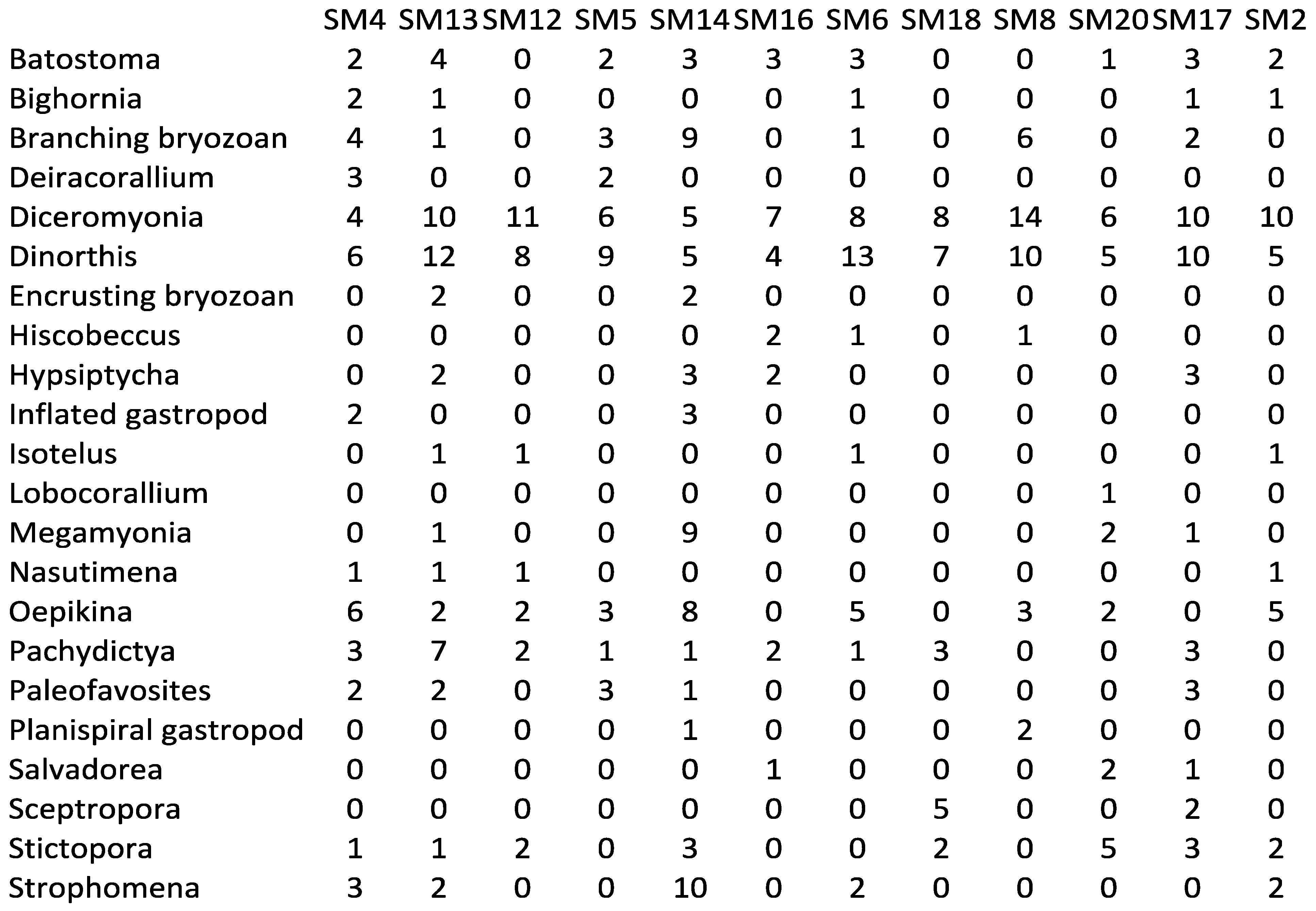
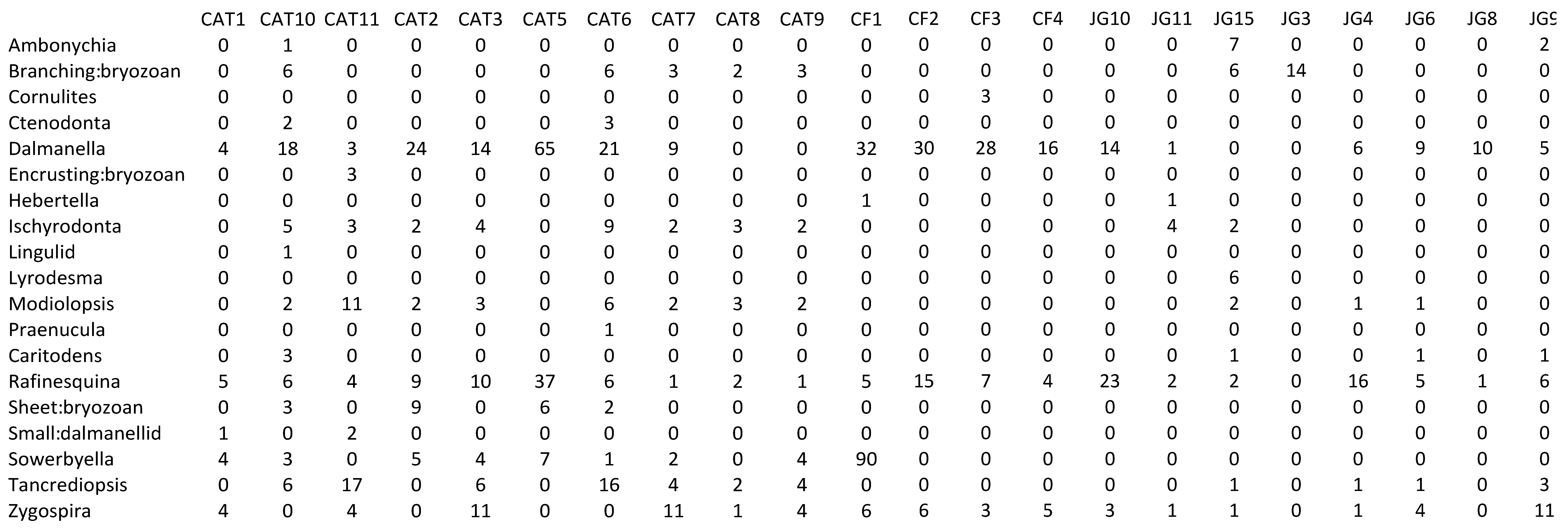
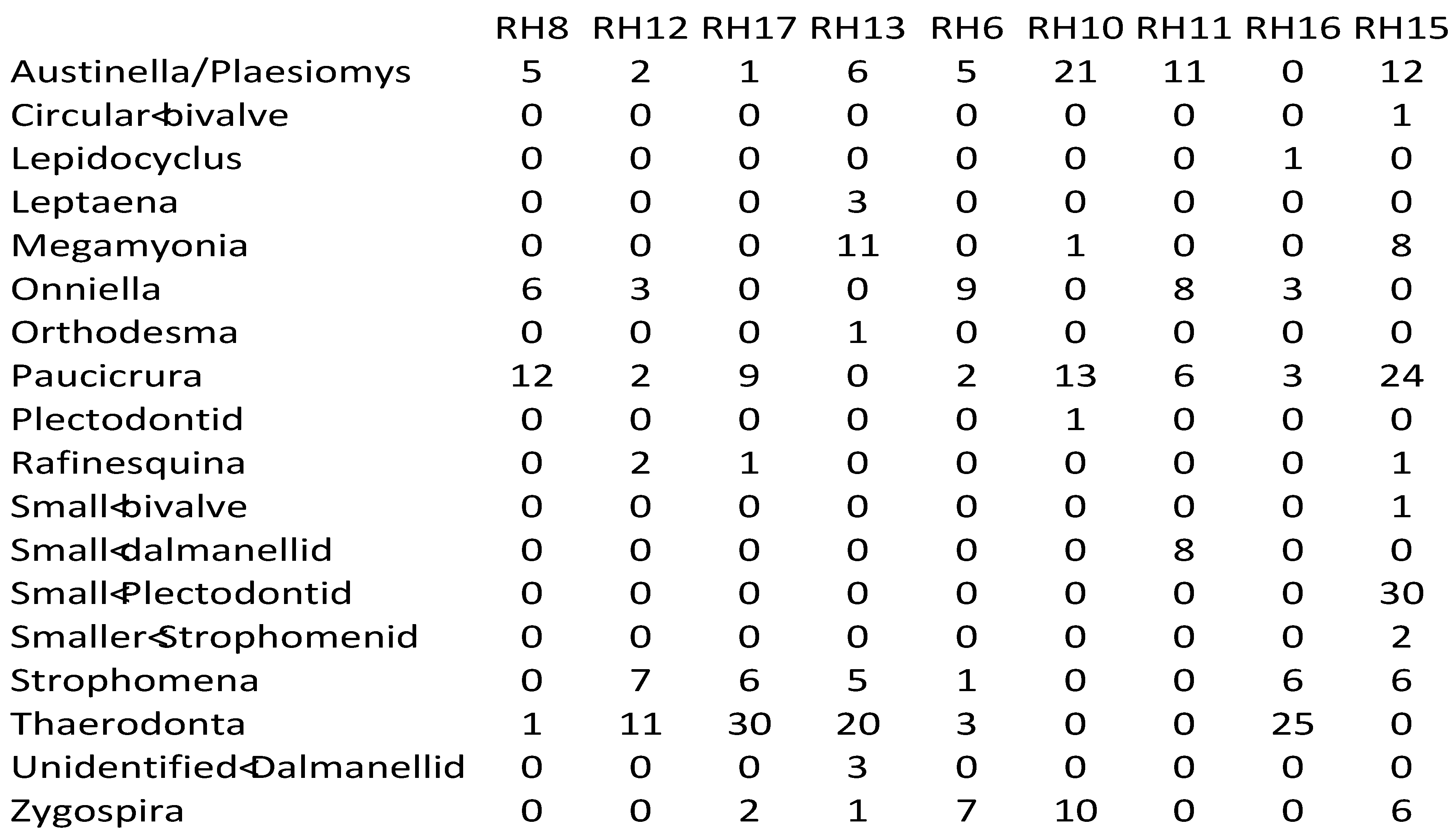
Appendix 2—Newly collected abundance data

Appalachian Basin (CAT: Catawba, CF: Catherine Furnace, JG: Germany Valley).
Diversity 05 00240 g010
Upper Mississippi Valley (RH: Rifle Hill Quarry).
Diversity 05 00240 g011
Manitoba (SM: Stony Mountain).
Diversity 05 00240 g012

