A Comparison of the Population Genetic Structure and Diversity between a Common (Chrysemys p. picta) and an Endangered (Clemmys guttata) Freshwater Turtle

Abstract

The northeastern United States has experienced dramatic alteration to its landscape since the time of European settlement. This alteration has had major impacts on the distribution and abundance of wildlife populations, but the legacy of this landscape change remains largely unexplored for most species of freshwater turtles. We used microsatellite markers to characterize and compare the population genetic structure and diversity between an abundant generalist, the eastern painted turtle (Chrysemys p. picta), and the rare, more specialized, spotted turtle (Clemmys guttata) in Rhode Island, USA. We predicted that because spotted turtles have disproportionately experienced the detrimental effects of habitat loss and fragmentation associated with landscape change, that these effects would manifest in the form of higher inbreeding, less diversity, and greater population genetic structure compared to eastern painted turtles. As expected, eastern painted turtles exhibited little population genetic structure, showed no evidence of inbreeding, and little differentiation among sampling sites. For spotted turtles, however, results were consistent with certain predictions and inconsistent with others. We found evidence of modest inbreeding, as well as tentative evidence of recent population declines. However, genetic diversity and differentiation among sites were comparable between species. As our results do not suggest any major signals of genetic degradation in spotted turtles, the southern region of Rhode Island may serve as a regional conservation reserve network, where the maintenance of population viability and connectivity should be prioritized.

1. Introduction

Rhode Island, a small state in the northeastern United States, has experienced intensive and large-scale landscape alteration in the last several centuries. Clearing of the land for timber and agriculture began in the 17th century and peaked in the mid-19th century, when approximately 70% of the state was deforested [1]. Freshwater wetlands have undergone immense alteration during this time, as well. Drainage, filling, damming, and channelization occurred for centuries without regulation, resulting in the loss of an estimated 37% of the wetlands in Rhode Island between 1780 and 1980 [2,3]. Undoubtedly, these human activities have had major impacts on the distribution, abundance, and connectivity of populations of wildlife throughout the state and region, but for most species the legacy of this change remains largely anecdotal or completely unexplored.

Populations of freshwater turtles in the region have certainly been impacted by these alterations, but not necessarily in a uniform fashion across species. Some species have experienced declines due primarily to historic habitat loss and fragmentation. True habitat specialists are often the most vulnerable and have probably experienced the most dramatic declines [4,5]. In contrast, habitat generalists have remained widespread and abundant owing to their ability to acclimate to new conditions, persist in heavily altered wetlands, and colonize manmade wetlands [6,7]. The eastern painted turtle (Chrysemys p. picta; hereafter painted turtle) and the spotted turtle (Clemmys guttata) are two species that are thought to have experienced very different responses to recent anthropogenic landscape change, with the former having remained abundant, and the latter having experienced substantial declines. In this study, we characterize and compare the population genetic diversity and the population genetic structure of the relatively rare spotted turtle with that of the more widespread and abundant painted turtle.

Painted turtles often occur in high abundance, even in areas of major human disturbance [8,9], and have been shown to occur in much higher densities than spotted turtles where they co-occur [10]. Eastern painted turtles are one of four recognized subspecies of C. picta, a small (carapace length up to 25.4 cm) freshwater turtle with a large geographic range that spans across North America [11]. The subspecies occupies the eastern part of this range, stretching from Georgia, USA to New Brunswick, Canada along the Atlantic seaboard. They occur in all types of freshwater wetlands including riparian systems. Sexual maturity usually occurs in 2–4 years in males, and 6–10 years in females [11]. Precise data are limited and variable across the range, but generation time is thought to be in the range of 10–20 years [11,12]. They are known to readily disperse from one wetland to another via terrestrial movements on the order of kilometers [13,14] and readily colonize uninhabited wetlands [15,16].

In contrast, spotted turtles are believed to have experienced severe population declines throughout their range in the last two centuries, due primarily to habitat loss, alteration, and fragmentation [17,18,19]. The spotted turtle is a small (carapace length up to 14.3 cm) freshwater turtle native to the eastern United States and the Great Lakes region [11]. Sexual maturity usually occurs between 7‒15 years [11] and tends to be at the higher end of this range in northern populations [20]. Estimates of generation time are usually considered to be between 20‒30 years, but may be as high as 40 years in the northern latitudes [11,21]. They are often described as semi-aquatic because they use both wetland and upland habitats for extended periods [22]. Throughout their range, spotted turtles occur in a variety of wetland types, but do exhibit habitat selection for shallow, bog-like wetlands [23,24]. In Rhode Island, spotted turtles are rare relative to other species of freshwater turtles and are strongly forest-associated [25]. Dispersal is limited and fidelity to wetlands is high, with individuals often returning to the same hibernaculum each winter [26,27]. They are a species of increasing conservation concern, especially in the northeastern United States where six of the seven states where the species occurs have designated it with some degree of conservation protection. The International Union for the Conservation of Nature (IUCN) currently lists the spotted turtle as Endangered [19], and it is currently under review by the U.S. Fish and Wildlife Service (USFWS) for federal listing under the U.S. Endangered Species Act [28].

Population genetics of endangered species are of fundamental interest to conservation biologists. Genetic diversity and inbreeding have implications for a population’s vulnerability to environmental and demographic stochasticity, thus affecting the probability of extinction [29,30]. A loss of genetic diversity can reduce the ability of a population to adapt to changing environmental conditions, and inbreeding depression can have deleterious effects on the reproductive fitness of offspring [31,32,33]. Genetic differentiation among subpopulations is, in part, a product of limited gene flow, and measures of differentiation can help identify subpopulations that may be genetically isolated due to barriers associated with habitat fragmentation. Maintaining gene flow to counteract the loss of genetic diversity due to inbreeding and genetic drift is an important management tactic to ensure genetic viability, especially for species that occur in small, isolated subpopulations [30].

Our primary objective was to assess whether spotted turtles in our study area exhibit genetic characteristics consistent with population declines, specifically, a reduction in genetic diversity, an increase in inbreeding, and greater population genetic structure due to isolation, which collectively we refer to as genetic degradation. We did this by comparing these characteristics in spotted turtles with the more common and abundant painted turtle. We made several predictions based on the insight that spotted turtles occur in smaller, more isolated populations, and that they probably exhibit reduced rates of gene flow compared to painted turtles. We predicted that spotted turtles would have (1) less genetic diversity, (2) higher inbreeding, (3) greater differentiation among sites, and (4) recently undergone reductions in effective population size (i.e., a population bottleneck), as compared to painted turtles.

2. Materials and Methods

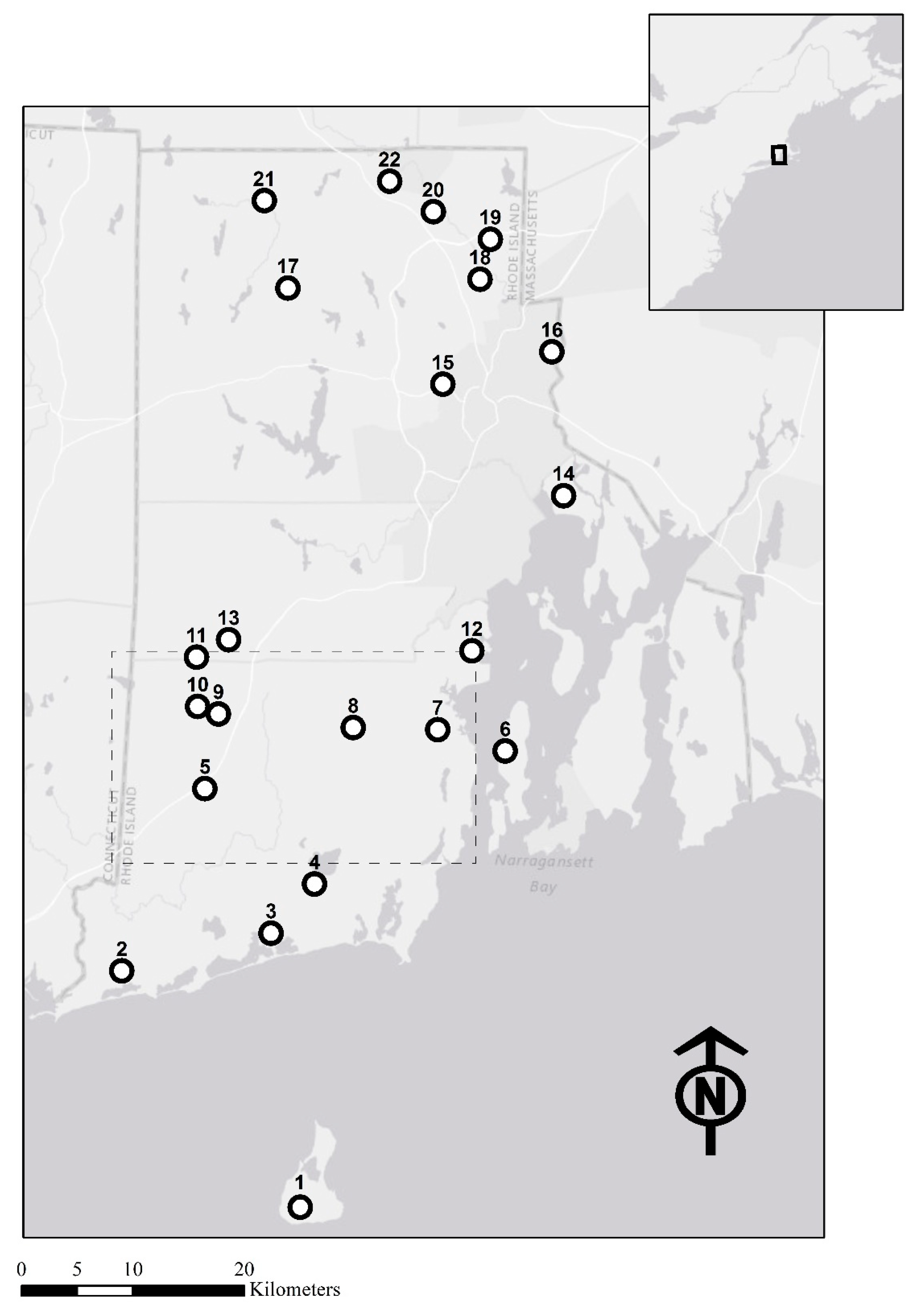
2.1. Study Area and Sampling

Our study was conducted throughout the state of Rhode Island located in southeastern New England. Rhode Island is the smallest state geographically in the United States (approximately 2700 square kilometers, when excluding coastal waterways), but ranks second highest in population density [34]. The highest levels of land development and human population densities occur along the south coast and around Narraganset Bay in the eastern part of the state. Approximately 54% of the state is forested, with pine, oak, and maple forests dominating the western part of the state [35]. Mean elevation is approximately 60 m, with a highest point of 247 m. Rhode Island experienced repeated glaciation during the Pleistocene Epoch, the most recent of which was the Laurentide Glacier. This glacier reached a terminus about 20 km south of Block Island between 21,000–24,000 years ago, and subsequently retreated northward leaving Rhode Island ice free by 16,000 years before present [36,37]. Today, Block Island is a 284 km² island located approximately 15 km south of the Rhode Island coast. Block Island has existed as an island for approximately 15,000 years since sea level rises associated with the retreat of the Laurentide Glacier caused the catastrophic drainage of glacial lakes along the southern New England terminal moraine [36].

From 2013–2015, small (0.1–1.8 ha), hydrologically isolated (i.e., discrete, non-riparian) wetlands throughout the state were randomly selected across a gradient of forest cover for a mark–recapture study focusing on occupancy and demography [25] (see reference for additional information on site selection and sampling methodology). Tissue collection for genetic analysis took place concurrently at a subset of these wetlands. Painted turtle tissue was collected from a group of wetlands that was representative of the conditions along this gradient and would ensure an adequate number of individuals for population genetics analysis [38]. One additional wetland was sampled for painted turtles on Block Island to serve as an outgroup. Because spotted turtles were relatively rare, tissue was collected from all individuals encountered during the study, and several additional wetlands known to contain the species were also sampled in order to augment the dataset. Two of these additional wetlands deviated from the other wetlands in notable ways. Site 24 was a slow-moving riparian wetland with peripheral freshwater marshes and adjacent forested vernal pools. Turtles were sampled from within an approximately 15 ha area that contained both the vernal pools and the riparian wetlands. Site 29 consisted of a matrix of permanent bog and forested vernal pools within a 2.5 ha area. Using historic aerial imagery, we determined that 6/33 (~18%) of the wetlands sampled were manmade or heavily modified after 1939, the year of the oldest available imagery [39]. These were sites 4, 7, 12, 15, 18, and 21. These did not include any of the wetlands where spotted turtles were sampled.

For all individuals, less than 1 mL of blood was collected from the sub-carapacial vein using a 25 gauge sterile needle and a 3 mL syringe and placed immediately on a Whatman FTA sample collection card (GE Healthcare, Buckinghamshire, UK). These cards were stored at room temperature and used for subsequent DNA extraction. All individuals were released at the site of capture. The Institutional Animal Care and Use Committee of the University of Rhode Island approved our methods (protocol #12–11–005). All work was carried out under scientific collecting permits (numbers 2013–12, 2014–25, and 2015–5) of the Rhode Island Department of Environmental Management.

2.2. Microsatellite Genotyping

We used the DNEasy Blood and Tissue Kit (Qiagen Corporation, Valencia, CA, USA) to extract DNA using the standard protocol. For both species, we amplified previously described microsatellite loci [40,41]. We amplified 18 loci for painted turtles and 17 loci for spotted turtles, organizing these into 6 and 5 multiplexes, respectively. We carried out polymerase chain reaction (PCR) using the Qiagen Type-it Microsatellite PCR Kit under the conditions recommended in King and Julian [41] but with a modified initial denaturing step of 95 °C for 5 min. We used negative controls on PCR plates to identify any potential contamination. Fragment size analysis of PCR products was conducted at the DNA Analysis Facility on Science Hill at Yale University on a 3730xl DNA Analyzer with a 96-capillary array, using GeneScan 600 LIZ dye size standard (Applied Biosystems, Foster City, CA, USA). Allele peaks were visualized and called using Geneious 7.0.6 [42]. We used Geneious and MICRO-CHECKER [43] to search for genotyping errors. We re-ran PCR and repeated genotyping for approximately 4% of our samples to calculate a genotyping error rate.

2.3. Genetic Diversity and Differentiation

We used a variety of packages developed for the R statistical platform v.3.3.3 [44] to estimate population genetic statistics. We used the poppr package [45] to quantify missing data and to test for linkage disequilibrium among loci. We used the pegas package [46] to test for deviations from Hardy-Weinberg Equilibrium (HWE) for each locus, and for each combination of locus and sampling site, using an exact test based on 10,000 Monte Carlo permutations of alleles. P-values were assessed after Bonferroni correction in which the alpha level (0.05) was divided by the number of tests. We used the popgenreport package [47] to estimate the frequency of null alleles for each locus [48], private alleles per site, and mean allelic richness using the rarefaction method to correct for variation in sample size [49]. We calculated expected heterozygosity (H_e), observed heterozygosity (H_o), and inbreeding coefficients (F_IS) for each site, and calculated 95% confidence intervals for F_IS estimates using 10,000 bootstrap iterations, all using the diveRsity package [50].

We used the diveRsity package to calculate the global measures of F_IS and F_ST, and to calculate pairwise F_ST values for all sites. All F-statistics used the bias-corrected formulation of Weir and Cockerham [51]. As an alternative measure of population differentiation and to maximize comparability with other studies, we also used the diveRsity package to calculate pairwise values of the bias-corrected Jost’s D_est [52,53]. The diveRsity package was used to estimate 95% confidence intervals for all measures of differentiation using 10,000 bootstrap iterations. We used the poppr package to perform an analysis of molecular variance (AMOVA). We conducted the test with two stratifications such that variance of allele frequencies was partitioned within and among sites [54]. For the global F-statistics and AMOVA analyses, we excluded the Block Island site for painted turtles, and included only the five spotted turtle sites with sample sizes >4 to limit confounding factors, such as outliers and small sample sizes [55], and thereby maximized the comparative inference between the two species.

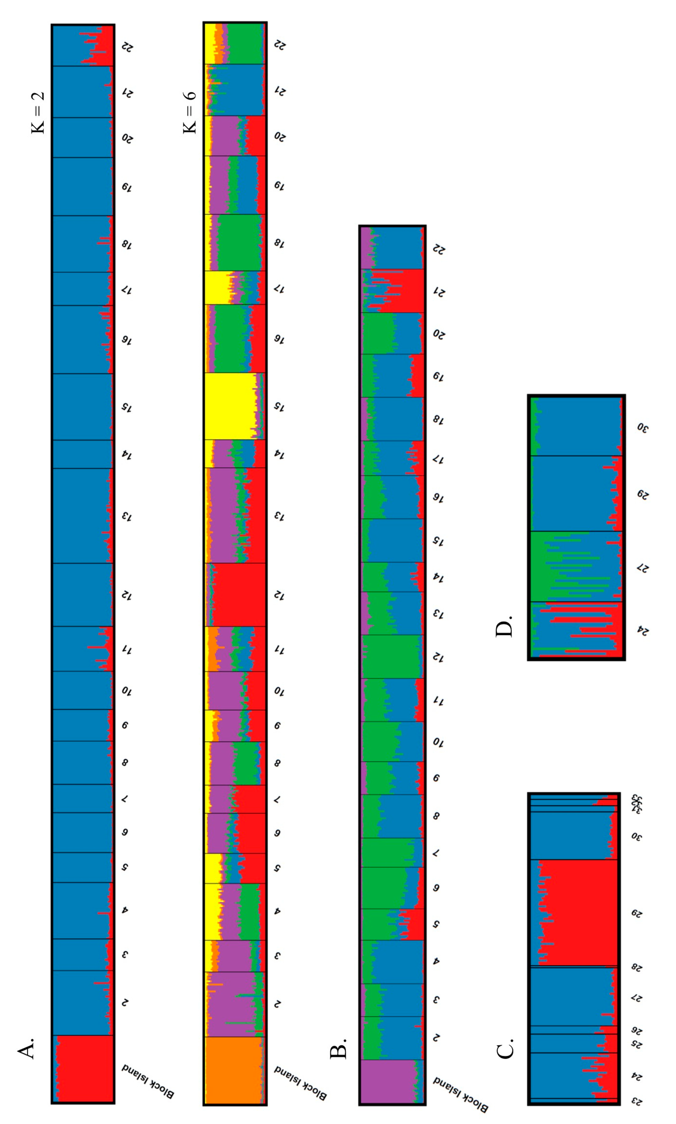
2.4. Population Structure

We used the ade4 package to perform a Mantel test with 10,000 permutations to test for genetic isolation by distance. We used Nei’s standard [56] measure of genetic distance to create the genetic matrix, and geographic locations centered on individual wetlands or on a geographic mean when turtles were sampled from multiple wetlands, to create the Euclidean distance matrix. For painted turtles, we did not include the Block Island site, and for spotted turtles we included only the five sites, with sample sizes >4 to avoid falsely inflating measures of genetic distance.

We used the program STRUCTURE v.2.3.4 [57] to characterize the population genetic structure of both species [58] and to test our prediction of a greater degree of subpopulation structure in spotted turtles. For all runs, we assumed an admixture model with correlated allele frequencies and employed the LOCPRIOR parameter using sampling location as the additional sample information. The LOCPRIOR parameter is informative in situations with weak population structure, such as that which may be expected given the spatial scale of our study [58,59]. In all cases, we performed 20 independent iterations of runs consisting of a burn-in of 200,000, followed by 500,000 MCMC repetitions, which was sufficient for all runs to reach convergence. For painted turtles, we ran an initial analysis with all individuals included (hereafter complete analysis) and a second analysis with a maximum of 25 individuals selected randomly (hereafter subset analysis) from each site to ensure that sample size unevenness was not influencing results [60]. We specified the range of K as 1–10 for both runs. For spotted turtles, we ran an initial analysis with all individuals from all sites (i.e., a complete analysis), and a second analysis with only sites with more than 9 individuals, while also limiting site 29 to only 30 randomly selected individuals (i.e., a subset analysis). We specified the range of K as 1–11 for the complete analysis, and 1–4 for the subset analysis. We considered both the ln Pr(X|K) and the ΔK method [61] with STRUCTURE Harvester [62] to evaluate the most likely number of clusters. We used CLUMPP v.1.1.2 [63] and distruct v.1.1 [64] software for post-hoc data processing and visualization.

2.5. Comparison of Pooled Groups

In order to more directly compare the genetic statuses of the two species, we created one geographically defined pooled group consisting of multiple sites, for each species. The geographic extent of the pooled groups was defined such that it would include the vast majority of spotted turtle samples and maximize the parity in sample size between the two species (Figure 1). For spotted turtles, this included sites 24, 25, 26, 27, 29, and 30. For painted turtles, this included sites 5, 7, 8, 9, 10, and 11. For each pooled group, we used the diveRsity package to estimate H_e, H_o, and F_IS, and used popgenreport to estimate mean allelic richness.

For each pooled group, we used the program BOTTLENECK v.1.2.02 [65] to test the prediction that spotted turtles were more likely than painted turtles to have undergone recent reductions in effective population size. To test for the signature of heterozygosity excess, we considered results from both a two-tailed sign test [66] and a one-tailed Wilcoxon signed-rank test using the two-phase mutation model (TPM), with 10,000 iterations used to generate a distribution of expected equilibrium heterozygosity. Following the recommendations of Peery et al. [67], we used a value of 3.1 for the mean size of multi-step mutations, which was used to specify a variance for the TPM [68]. We then conducted separate tests using values of 0.05, 0.15, 0.25, and 0.35 for the proportion of multi-step mutations in the TPM. To estimate the effective population size (N_e) for each pooled group, we used the program NeEstimator v.2.1 [69], using the linkage disequilibrium method under the assumption of random mating. We performed estimates using all possible alleles, and excluding alleles with a frequency <0.05. We report both parametric and jackknife 95% confidence intervals for all estimates.

3. Results

3.1. Sampling and Genotyping

We collected tissue samples from 647 painted turtles from 22 sites (mean = 29.7 individuals/site, SE = 2.2), and 148 spotted turtles from 11 sites, but only five of these 11 sites yielded enough individuals for the majority of population genetics analyses (mean = 27.4 individuals/site, SE = 6.4, n = 5; Figure 1 and Figure 2). We retained 12 of 18 microsatellite loci for painted turtles (Table S1). Excluded loci were GmuB67 and GmuA32, which were monomorphic, GmuD87 and Cp10, which had high levels of missing data (> 13%) and high frequencies of null alleles (0.120 and 0.219, respectively), and loci GmuD121 and Cp2, which had high frequencies of null alleles (0.205 and 0.158, respectively). GmuD87, GmuD121, and Cp10 deviated most consistently from HWE among the sampling sites (Figure S1). For retained loci, the total missing data was 3.6%. We retained 16 of 17 loci for spotted turtles (Table S1). We removed the locus GmuD28, which had a high frequency of null alleles (0.174). For the retained loci, the total missing data was 0.6%. There was no evidence of linkage disequilibrium among retained loci for either species. The genotyping error rate was approximately 2.3%.

3.2. Genetic Diversity and Population Structure

Painted turtle global F_IS was less than zero (−0.0220, CI = −0.0341–−0.0099), and global F_ST was greater than zero (0.0185, CI = 0.0143–0.0231). For this species, mean H_e of all retained loci was 0.66 (SE = 0.08) and mean H_o was 0.66 (SE = 0.08; Table S1). Mean allelic richness ranged from 5.54 to 6.59 among sites (

Table 1. Site characteristics and genetic diversity measures for painted turtles and spotted turtles in Rhode Island, USA, 2013–2015.

Site	Geographic Coordinates (Latitude, Longitude)	No. of Individuals	He	Ho	Private Alleles	Mean Allelic Richness	FIS
Painted turtles
1	41.153247, −71.604493	40	0.63	0.63	2	5.83	0.014
2	41.346108, −71.789074	39	0.61	0.60	0	6.21	−0.012
3	41.380141, −71.630523	19	0.61	0.67	1	5.82	−0.101
4	41.42052, −71.585525	34	0.63	0.66	0	6.29	−0.062
5 *	41.494763, −71.706265	18	0.61	0.66	1	5.69	−0.076
6	41.53227, −71.385252	24	0.59	0.59	0	5.54	−0.003
7 *	41.548007, −71.458184	17	0.59	0.63	0	5.75	−0.076
8 *	41.547675, −71.549071	26	0.63	0.64	2	6.59	−0.022
9 *	41.555359, −71.694297	19	0.63	0.71	1	6.33	−0.127
10 *	41.560943, −71.716856	23	0.63	0.64	0	6.22	−0.018
11 *	41.600674, −71.719651	27	0.65	0.68	0	6.21	−0.058
12	41.612399, −71.42399	38	0.64	0.69	0	5.96	−0.073
13	41.615407, −71.685647	57	0.62	0.63	1	6.34	−0.029
14	41.739527, −71.329793	17	0.62	0.67	0	5.79	−0.065
15	41.826773, −71.463335	40	0.62	0.60	2	6.02	0.034
16	41.855324, −71.346786	41	0.64	0.63	1	6.54	0.016
17	41.900587, −71.633623	20	0.63	0.69	0	6.25	−0.100
18	41.912204, −71.426565	34	0.61	0.61	0	6.18	−0.005
19	41.944757, −71.416485	35	0.65	0.71	0	6.29	−0.090
20	41.965696, −71.478915	24	0.62	0.67	0	6.12	−0.078
21	41.970512, −71.66193	31	0.64	0.68	0	5.94	−0.064
22	41.98915, −71.527097	24	0.59	0.61	2	5.98	−0.018
Global values		607	-	-	-	-	−0.022
Pooled group	-	130	0.64	0.66	-	10.27	−0.026
Spotted turtles
23	-	2	-	-	1	-	-
24 *	-	22	0.65	0.63	2	4.78	0.040
25 *	-	9	0.67	0.68	2	4.81	−0.028
26 *	-	4	-	-	1	-	-
27 *	-	28	0.67	0.67	3	4.86	−0.008
28	-	1	-	-	1	-	-
29 *	-	51	0.67	0.64	5	4.90	0.033
30 *	-	23	0.68	0.67	6	4.97	0.007
31	-	3	-	-	1	-	-
32	-	3	-	-	1	-	-
33	-	2	-	-	1	-	-
Global values	-	133	-	-	-	-	0.036
Pooled group	-	137	0.68	0.66	-	8.59	0.039

Geographic coordinates are in decimal degrees (locations withheld for spotted turtles). H_e is expected heterozygosity, H_o is observed heterozygosity, and F_IS is the inbreeding coefficient. Bolded F_IS indicates a bootstrapped 95% confidence interval that does not overlap zero. Diversity measures (except private alleles) calculated only for sampling sites with >4 individuals for spotted turtles. Asterisks indicate a site used to compile the pooled group for each species.

). Pairwise F_ST values (not including Block Island) ranged from 0.002 to 0.058 (mean = 0.018, SE = 0.001, n = 210), with 143/210 (68.1%) values containing a 95% confidence interval that did not overlap zero. Only the Block Island site (F_ST = 0.008–0.081) and sites 12 (F_ST = 0.019–0.058) and 21 (F_ST = 0.019–0.055) contained all values that did not overlap zero (Table S2). Pairwise Jost’s D_est values ranged from 0.001 to 0.102 (mean = 0.020, SE = 0.001, n = 210), with 51/210 (24.3%) of values containing a 95% confidence interval that did not overlap zero.

Spotted turtle global F_IS (0.0364, CI = 0.0094–0.0628) and F_ST (0.0144, CI = 0.0045–0.0264) were greater than zero. For this species, mean H_e of all retained loci was 0.70 (SE = 0.04) and mean H_o was 0.68 (SE = 0.05; Table S1). Mean allelic richness ranged from 4.78 to 4.97 among sites (Table 1). Pairwise F_ST values ranged from −0.002 to 0.025 (mean = 0.012, SE = 0.003, n = 10), and 3/10 (30%) values contained a 95% confidence interval that did not overlap zero. Pairwise Jost’s D_est values ranged from 0 to 0.031 (mean = 0.010, SE = 0.003, n = 10), and 1/10 values (10%) contained a 95% confidence interval that did not overlap zero (Table S3).

The vast majority of genetic variance occurred within sites for both species (AMOVA: painted turtle = 96.5%; spotted turtle = 97.9%), with the remaining variance partitioned among sites, and we found no evidence for isolation by distance in painted turtles (r = 0.097, p = 0.128, 21 sites) or spotted turtles (r = −0.454, p = 0.926, 5 sites). STRUCTURE results for painted turtles clearly distinguished the Block Island site from all mainland sampling locations in all runs. In the complete analysis, the ΔK method suggested two clusters, and the ln Pr(X|K) method suggested six clusters. In the subset analysis, both K selection methods suggested four clusters (Figure 2A,B; Figure S2). In both analyses in which K ≥ 4, the majority of sites showed a lack of definitive assignment of individuals to a particular cluster, but several sites did show a relatively high probability of assignment to a particular cluster. In the complete analysis, sites 2, 12, 15, 18, and 21 exhibited the highest probabilities of belonging to independent clusters. In the subset analysis, sites 12, 15, and 21 exhibited the highest probabilities of belonging to independent clusters. STRUCTURE results for spotted turtles suggested two genetic clusters in the complete analysis, with site 29 distinguished from the other sites. In the subset analysis, this relationship did not persist and the ΔK and ln Pr(X|K) methods suggested different numbers of clusters (Figure 2C–D; Figure S2). The ln Pr(X|K) method suggested no structure (i.e, K = 1), and the ΔK method suggested three clusters with a greater amount of admixture in sites 24 and 27.

3.3. Comparison of Pooled Groups

For the painted turtle pooled group, H_e was 0.64, H_o was 0.66, F_IS was −0.026 (−0.051–−0.001), and mean allelic richness was 10.27. For the spotted turtle pooled group, H_e was 0.68, H_o was 0.66, F_IS was 0.039 (0.015–0.064), and mean allelic richness was 8.59 (Table 1). Painted turtles exhibited no evidence of a recent genetic bottleneck, with all tests returning non-significant results. For spotted turtles, both the sign test and Wilcoxon test at the highest TPM level returned P-values <0.05, suggesting the signal of a recent population decline (

Table 2. Results from program BOTTLENECK for pooled groups of painted turtles and spotted turtles showing P-values of sign tests and Wilcoxon signed-rank tests under varying proportions of multi-step mutation model included in the two-phase model. Asterisk indicates P-value < 0.05.

	Proportion of Multi-Step Mutation Model
	0.05		0.15		0.25		0.35
Species	Sign Test	Wilcoxon Test	Sign Test	Wilcoxon Test	Sign Test	Wilcoxon Test	Sign Test	Wilcoxon Test
Painted turtles	0.586	0.545	0.337	0.425	0.331	0.395	0.322	0.259
Spotted turtles	0.505	0.550	0.478	0.161	0.477	0.072	0.048 *	0.017 *

). Estimates of effective population size were higher for painted turtles, especially when all alleles were included in the analysis, but there was substantial overlap in confidence intervals between the two species (

Table 3. Results from program NeEstimator showing effective population size estimates (N_e) and 95% confidence intervals (CI) for painted turtle and spotted turtle pooled groups.

Critical Value	Ne	Parametric 95% CI	Jack-Knife 95% CI	Ne	Parametric 95% CI	Jack-Knife 95% CI
	Painted turtles			Spotted turtles
0.05	283.3	174–642.3	132–4387.4	242.1	175.3–371.9	141.9–611.5
All alleles	692.9	395.6–2354.3	237.2–Infinite	334.9	255.7–473.8	206.7–756.7

).

4. Discussion

Measures of genetic diversity were mixed, with observed heterozygosity similar for both species, but spotted turtles exhibited a lower allelic richness. Population genetic structure was comparable for both species, highlighted by little differentiation among sites and no evidence of isolation by distance for either species. However, it should be noted that the Mantel test for spotted turtles included only five sites, thereby limiting the statistical power of the test and our ability to detect a trend. For painted turtles, both global and pooled group F_IS was less than zero, suggesting outbreeding. For spotted turtles, however, global and pooled group F_IS was greater than zero, indicating a modest amount of inbreeding. There was tentative evidence of a recent population decline in the spotted turtle pooled group, whereas there was no evidence of a population decline in the painted turtle pooled group. Overall, the results were consistent with some predictions and inconsistent with others. We interpret this as limited evidence that the spotted turtle has experienced some, albeit modest, genetic degradation in our study area.

4.1. Genetic Diversity

Lower mean allelic richness in spotted turtles suggests less genetic diversity compared to painted turtles, yet the observed heterozygosity was identical in the two pooled groups. For both species, estimates of observed and expected heterozygosity and allelic richness were comparable to those from other studies of turtles using microsatellites [70], which suggests no significant depletion of genetic diversity. However, long-lived species can mask declines in genetic diversity even after prolonged population declines, making interpretation difficult [71]. A comparison of genetic diversity in fragmented populations of spotted turtles and midland painted turtles (C. picta marginata) in Indiana found lower diversity in spotted turtles [72]. The authors identify a smaller habitat patch size, lower population density, and greater isolation of spotted turtle populations as potential factors, but low sample sizes and the possibility of different mutation rates of the genetic markers used for the different species limit strong conclusions from this study. In a Wisconsin study, genetic diversity was highest in painted turtles, intermediate in snapping turtles (Chelydra serpentina), and lowest in Blanding’s turtles (Emydoidea blandingii) [73]. This was consistent with the prediction that genetic diversity would decrease with reduced mobility and greater habitat specialization among these turtle species. A study comparing the same three species in Illinois yielded similar results, with populations of Blanding’s turtles, snapping turtles, and painted turtles exhibiting increasing allelic richness and heterozygosity, respectively [74]. The study in Illinois did not detect intraspecific differences between fragmented and relatively undisturbed sites, however. While some studies have demonstrated strong empirical evidence of a relationship between genetic diversity, life history, and the landscape, it remains difficult to compare genetic diversity directly between species when different loci are used, as these loci can influence estimates [75,76]. Standardized approaches for comparing genetic diversity among species and studies are needed so that conservation scientists can better resolve causality for this important measure.

4.2. Population Structure

We documented weak, but existing, differentiation among some painted turtle sampling sites. The Block Island site was only moderately differentiated, despite very limited opportunity for gene flow with the mainland since the Pleistocene [77]. The post-glacial colonization of the northeastern United States by painted turtles occurred as populations expanded from southern refugia after glaciers retreated [78]. Painted turtles are physiologically well adapted to cold climates [79,80] and, along with snapping turtles, were the first turtles to expand northward into formerly glaciated areas [81]. The exact time at which these species first colonized what is now Block Island and mainland Rhode Island is not known, but it probably took place between 10,000 and 15,000 years ago [78,81]. A characteristic reduction in genetic diversity associated with this relatively recent post-glacial range expansion [82,83], along with high rates of contemporary gene flow, may be responsible for the lack of pronounced population genetic structure.

The STRUCTURE results indicated that the majority of painted turtle sites were assigned to multiple genetic clusters, a common signature of weak population structure [58]. However, sites 12, 15, and 21 did exhibit consistent signals of substructure, both in pairwise measures of differentiation and in STRUCTURE results. Under both scenarios where K ≥ 4, these sites contained the highest probabilities of belonging to the distinct clusters (Figure 2A–B). Interestingly, these three sites are all manmade or heavily modified [25]. Sites 12 and 15 were both constructed between 1972 and 1976, whereas site 21 predates the earliest available aerial imagery but is clearly a pool that formed when a former stream was bisected by a road. These three sites also contain plentiful nesting habitats immediately adjacent to the wetland. Recent colonization by a small number of individuals (i.e., a founder effect), followed by a rapid expansion in population size due to recruitment, may be responsible for this marked differentiation. Ultimately, however, we cannot say with certainty what is causing the observed genetic distinctiveness of these populations. Future studies comparing population genetics in manmade and natural wetlands would be instructive.

Contrary to our predictions, we detected very little differentiation among spotted turtle sites. In fact, a smaller percentage of sites exhibited significant pairwise differentiation compared to painted turtles, but direct comparison is difficult because of the disparity in sample size (spotted turtle = 20 pairwise comparisons, painted turtle = 420 pairwise comparisons). All significant spotted turtle pairwise comparisons included site 29 and this site was also differentiated in the complete STRUCTURE analysis. Adults from site 29 were radiotracked for two years as part of another study and were found to exhibit limited movements and high levels of home range fidelity [84]. Given that dispersal is a requisite process for gene flow, if dispersal rates to neighboring wetlands are indeed low, limited gene flow could explain the higher differentiation. The spotted turtle STRUCTURE subset analysis resulted in a more ambiguous pattern of differentiation, and the fact that the ΔK and ln Pr(X|K) methods resulted in disparate results makes this difficult to interpret.

4.3. Population Bottleneck and Effective Population Size

We documented tentative evidence for a recent population decline in the pooled group of spotted turtles. We ran multiple tests under a range of different multi-step mutation model proportions to assess the robustness of the results [67]. Statistical evidence for a population bottleneck occurred at the higher proportion of the multi-step model in the TPM, where the test is most vulnerable to Type I error [68]. Thus, our results should be interpreted with caution. Bottleneck tests can be difficult to interpret, but results comparable to ours have been interpreted in a similar way as those for other species of turtles [71].

Due to overlapping and sometimes wide confidence intervals, the interpretation of effective population size estimates for the pooled groups proved difficult. Estimates for painted turtles were higher, especially under the all alleles scenario in which the painted turtle estimate was more than double that of the spotted turtle estimate. However, a jack-knife 95% confidence interval that has no upper limit precludes clear interpretation.

4.4. Scope and Limitations

For both species, the magnitude of the genetic structure that we did detect was very modest. Given the limited spatial scale of our study and the fact that we expected these sampling sites to be of post-Pleistocene origin and feature admixing to some degree, it should be emphasized that we were indeed seeking fine-scale genetic structure. Moreover, in our study area, the impact of human activities we intended to explore has occurred in the evolutionarily recent past (~250 years) and intensified only in the last ~75 years. The number of painted turtle generations since the more intense period of human influence began is probably 4–7 generations and 12–25 generations for the longer period. The number of spotted turtle generations is probably 2–4 for the shorter period and 8–12 for the longer period. As it can be difficult to detect the effects of genetic drift in long-lived organisms, the spatial and temporal scales (i.e., time since habitat loss and fragmentation) of our investigation may have limited our ability to detect genetic differentiation and demographic events that have occurred in the recent past, particularly for spotted turtles, given their longer generation time and the smaller geographic range from which they were sampled.

Simulation studies have demonstrated that F_ST is relatively insensitive to disruptions in gene flow, especially when dispersal is limited and that other population-based metrics may be superior in detecting changes that have occurred in the recent past [85]. Compounding the issue, turtle DNA mutates slowly relative to that of other vertebrates [86,87]. Other studies of population genetics in freshwater turtles have failed to detect predicted genetic structure, even when there is strong empirical evidence of the effects of historic habitat fragmentation [74,88]. Nonetheless, the ability to detect strong genetic structure among sites in as few as 1–10 generations after fragmentation has been demonstrated in reptiles [89,90,91]. Given an ample number of generations, the same should be possible in turtles, but it is not yet clear how many generations are necessary, and this number likely varies among species. When working on such limited spatial and temporal scales, adequate sample size, number of markers used, and mutation rates of markers need to be considered to maximize the resolution of analyses [38,55,92,93]. Direct comparisons among studies can also be difficult, and standardized approaches and accepted minimums of markers and sample sizes would be helpful in improving the interpretability and context of individual studies.

5. Conclusions

Painted turtles are one of the most well-studied freshwater turtle species, largely because they are widespread and abundant. Our analysis confirms that they exhibit little population genetic structure across Rhode Island, making for an appropriate contrast with a far less abundant species. Some sites did exhibit modest genetic differentiation, but the reasons why remain elusive and warrant further investigation. Our study suggests that spotted turtles exhibit little population genetic structure at the spatial scale explored. These results reinforce that, from a genetic perspective, these species should be managed as contiguous populations at the landscape scale and that future studies of population genetics in freshwater turtles that wish to delineate differentiation should be carried out at an appropriately large scale.

Our analysis provides some evidence that spotted turtles have experienced a greater degree of inbreeding and may have experienced population declines in the recent past in our study area. However, overall, diversity and population genetic structure in this species remain comparable to that of painted turtles. As we were unable to find strong evidence for genetic degradation in spotted turtles, the southern region of Rhode Island may be well suited to serve as a regional conservation reserve network where the maintenance of populations and connectivity among wetlands should be prioritized [94,95]. Relatively little is known about spotted turtle population genetics and how genetic structure varies range-wide. Much of what has been inferred is derived from studies of different species of freshwater turtles considered ecologically similar. Understanding the legacy, significant or not, of habitat loss and fragmentation on population genetic structure is critical for effective management and conservation of this species. Additional population genetic studies, at both local and regional scales, will help improve our understanding of the potential vulnerabilities to environmental and genetic stochasticity in this species of conservation concern.

References

1. Foster, D.R.; Aber, J.D. Forests in Time: The Environmental Consequences of 1000 years of Change in New England; Yale University Press: New Haven, CT, USA, 2004; ISBN 9780300115376. [Google Scholar]
2. Dahl, T.E. Wetlands Losses in the United States, 1780’s to 1980’s; U.S. Department of the Interior, Fish and Wildlife Service: Washington, DC, USA, 1990; 13p.
3. Magilligan, F.J.; Graber, B.E.; Nislow, K.H.; Chipman, J.W.; Sneddon, C.S.; Fox, C.A. River restoration by dam removal: Enhancing connectivity at watershed scales. Elementa 2016, 4, 000108. [Google Scholar] [CrossRef] [Green Version]
4. U.S. Fish and Wildlife Service. Bog Turtle (Clemmys muhlenbergii), Northern Population, Recovery Plan; U.S. Fish and Wildlife Service: Hadley, MA, USA, 2001; 103p.
5. Rosenbaum, P.A.; Robertson, J.M.; Zamudio, K.R. Unexpectedly low genetic divergences among populations of the threatened bog turtle (Glyptemys muhlenbergii). Conserv. Genet. 2007, 8, 331–342. [Google Scholar] [CrossRef]
6. Price, S.J.; Guzy, J.C.; Witczak, L.; Dorcas, M.E. Do ponds on golf courses provide suitable habitat for wetland-dependent animals in suburban areas? An assessment of turtle abundances. J. Herpetol. 2013, 47, 243–250. [Google Scholar] [CrossRef]
7. Winchell, K.M.; Gibbs, J.P. Golf courses as habitat for aquatic turtles in urbanized landscapes. Landsc. Urban Plan. 2016, 147, 59–70. [Google Scholar] [CrossRef]
8. Congdon, J.D.; Gibbons, J.W. Structure and Dynamics of a Turtle Community. In Long-Term Studies of Vertebrate Communities; Cody, M.L., Smallwood, J.A., Eds.; Academic Press: San Diego, CA, USA, 1996; pp. 137–159. [Google Scholar]
9. Gamble, T.; Simons, A.M. Comparison of harvested and nonharvested painted turtle populations. Wildl. Soc. Bull. 2004, 32, 1269–1277. [Google Scholar] [CrossRef] [Green Version]
10. Ernst, C.H. Ecology of the spotted turtle, Clemmys guttata (Reptilia, Testudines, Testudinidae), in southeastern Pennsylvania. J. Herpetol. 1976, 10, 25–33. [Google Scholar] [CrossRef]
11. Ernst, C.H.; Lovich, J.E. Turtles of the United States and Canada, 2nd ed.; John Hopkins University Press: Baltimore, MD, USA, 2009; ISBN 9780801891212. [Google Scholar]
12. Wilbur, H.M. The evolutionary and mathematical demography of the turtle Chrysemys picta. Ecology 1975, 56, 64–77. [Google Scholar] [CrossRef]
13. Zweifel, R.G. Long–term ecological studies on a population of painted turtles, Chrysemys picta, on Long Island, New York. Am. Mus. Novit. 1989, 2952, 1–55. [Google Scholar]
14. Bowne, D.R. Terrestrial activity of Chrysemys picta in Northern Virginia. Copeia 2008, 2008, 306–310. [Google Scholar] [CrossRef]
15. Tuberville, T.D.; Gibbons, J.W.; Greene, J.L. Invasion of new aquatic habitats by male freshwater turtles. Copeia 1996, 1996, 713–715. [Google Scholar] [CrossRef]
16. Cosentino, B.J.; Schooley, R.L.; Phillips, C.A. Wetland hydrology, area, and isolation influence occupancy and spatial turnover of the painted turtle, Chrysemys picta. Landsc. Ecol. 2010, 25, 1589–1600. [Google Scholar] [CrossRef]
17. Gibbons, J.W.; Scott, D.E.; Ryan, T.J.; Buhlmann, K.A.; Tuberville, T.D.; Metts, B.S.; Greene, J.L.; Mills, T.; Leiden, Y.; Poppy, S.; et al. The global decline of reptiles, déjà vu amphibians. BioScience 2000, 50, 653–666. [Google Scholar] [CrossRef]
18. Lewis, T.L.; Ulmer, J.M.; Mazza, J.L. Threats to spotted turtle (Clemmys guttata) habitat in Ohio. Ohio J. Sci. 2004, 104, 65–71. [Google Scholar]
19. Van Dijk, P.P. Clemmys guttata. The IUCN Red List of Threatened Species. e.T4968A97411228. 2011. Available online: http://dx.doi.org/10.2305/IUCN.UK.2011-1.RLTS.T4968A11103766.en (accessed on 15 January 2013).
20. Litzgus, J.D.; Brooks, R.J. Growth in a cold environment: Body size and sexual maturity in a northern population of spotted turtles, Clemmys guttata. Can. J. Zool. 1998, 76, 773–782. [Google Scholar] [CrossRef]
21. COSEWIC. COSEWIC Assessment and Update Status Report on Spotted Turtle Clemmys guttata in Canada; Committee on the Status of Endangered Wildlife in Canada Ottawa: Ottawa, ON, USA, 2014; 74p. [Google Scholar]
22. Beaudry, F.; deMaynadier, P.G.; Hunter, M.L. Seasonally dynamic habitat use by spotted (Clemmys guttata) and blanding’s turtles (Emydoidea blandingii) in Maine. J. Herpetol. 2009, 43, 636–645. [Google Scholar] [CrossRef]
23. Milam, J.C.; Melvin, S.M. Density, habitat use, movements, and conservation of spotted turtles (Clemmys guttata) in Massachusetts. J. Herpetol. 2001, 35, 418–427. [Google Scholar] [CrossRef]
24. Rasmussen, M.L.; Litzgus, J.D. Habitat selection and movement patterns of spotted turtles (Clemmys guttata): Effects of spatial and temporal scales of analyses. Copeia 2010, 2010, 86–96. [Google Scholar] [CrossRef]
25. Buchanan, S.W.; Buffum, B.; Puggioni, G.; Karraker, N.E. Occupancy of freshwater turtles across a gradient of altered landscapes. J. Wildl. Manag. 2019, 83, 435–445. [Google Scholar]
26. Haxton, T.; Berrill, M. Habitat selectivity of Clemmys guttata in central Ontario. Can. J. Zool. 1999, 77, 593–599. [Google Scholar] [CrossRef]
27. Litzgus, J.D.; Costanzo, J.P.; Brooks, R.J.; Lee, J.R.E. Phenology and ecology of hibernation in spotted turtles (Clemmys guttata) near the northern limit of their range. Can. J. Zool. 1999, 77, 1348–1357. [Google Scholar]
28. U.S. Fish and Wildlife Service. Petition to List Spotted Turtle in Connecticut, Delaware, Florida, Georgia, Illinois, Maine, Maryland, Massachusetts, Michigan, Pennsylvania, New Hampshire, New York, North Carolina, Ohio, South Carolina, Vermont, Virginia, and West Virginia under the Endangered Species Act of 1973; as Amended; Federal Register Docket ID FWS–R5–ES–2015–0064; U.S. Fish and Wildlife Service: Washington, DC, USA, 2015.
29. Brook, B.W. Demographics Versus Genetics in Conservation Biology. In Conservation Biology: Evolution in Action; Carroll, S.P., Fox, C.W., Eds.; Oxford University Press: New York, NY, USA, 2008; pp. 35–49. ISBN 978-0195306781. [Google Scholar]
30. Frankham, R.; Ballou, J.D.; Briscoe, D.A. Introduction to Conservation Genetics; Cambridge University Press: Cambridge, UK, 2010; ISBN 978-0521702713. [Google Scholar]
31. Ralls, K.; Ballou, J.D.; Templeton, A. Estimates of lethal equivalents and the cost of inbreeding in mammals. Conserv. Biol. 1988, 2, 185–193. [Google Scholar] [CrossRef]
32. Frankham, R. Genetics and extinction. Biol. Conserv. 2005, 126, 131–140. [Google Scholar] [CrossRef]
33. O’Grady, J.J.; Brook, B.W.; Reed, D.H.; Ballou, J.D.; Tonkyn, D.W.; Frankham, R. Realistic levels of inbreeding depression strongly affect extinction risk in wild populations. Biol. Conserv. 2006, 133, 42–51. [Google Scholar] [CrossRef]
34. U.S. Census Bureau. Population, Housing Units, Area, and Density: 2010. 2010. Available online: https://factfinder.census.gov (accessed on 15 January 2013).
35. Butler, B.J. Rhode Island’s Forest Resources, 2012; Res. Note, NRS-190; U.S. Forest Service: Newton Square, PA, USA, 2013; 3p.
36. Uchupi, E.; Driscoll, N.; Ballard, R.D.; Bolmer, S.T. Drainage of late Wisconsin glacial lakes and the morphology and late quaternary stratigraphy of the New Jersey–southern New England continental shelf and slope. Mar. Geol. 2001, 172, 117–145. [Google Scholar] [CrossRef]
37. Boothroyd, J.C.; Sirkin, L. Quaternary geology and landscape development of Block Island and adjacent regions. In Proceedings of the Rhode Island Natural History Survey, Kingston, RI, USA, 28 October 2000; pp. 13–27. [Google Scholar]
38. Hale, M.L.; Burg, T.M.; Steeves, T.E. Sampling for microsatellite-based population genetic studies: 25 to 30 individuals per population is enough to accurately estimate allele frequencies. PLoS ONE 2012, 7, e45170. [Google Scholar] [CrossRef] [PubMed]
39. Rhode Island Geographic Information System Home Page. Available online: http://www.rigis.org/ (accessed on 1 February 2013).
40. Pearse, D.E.; Janzen, F.J.; Avise, J.C. Genetic markers substantiate long-term storage and utilization of sperm by female painted turtles. Heredity 2001, 86, 378–384. [Google Scholar] [CrossRef] [PubMed]
41. King, T.L.; Julian, S.E. Conservation of microsatellite DNA flanking sequence across 13 Emydid genera assayed with novel bog turtle (Glyptemys muhlenbergii) loci. Conserv. Genet. 2004, 5, 719–725. [Google Scholar] [CrossRef]
42. Kearse, M.; Moir, R.; Wilson, A.; Stones-Havas, S.; Cheung, M.; Sturrock, S.; Buxton, S.; Cooper, A.; Markowitz, S.; Duran, C. Geneious Basic: An integrated and extendable desktop software platform for the organization and analysis of sequence data. Bioinformatics 2012, 28, 1647–1649. [Google Scholar] [CrossRef]
43. Van Oosterhout, C.; Hutchinson, W.F.; Wills, D.P.; Shipley, P. MICRO-CHECKER: Software for identifying and correcting genotyping errors in microsatellite data. Mol. Ecol. Resour. 2004, 4, 535–538. [Google Scholar] [CrossRef]
44. R Core Team. R: A Language and Environment for Statistical Computing; R Foundation for Statistical Computing: Vienna, Austria, 2017; Available online: http://www.R-project.org/ (accessed on 15 January 2018).
45. Kamvar, Z.N.; Tabima, J.F.; Grünwald, N.J. Poppr: An R package for genetic analysis of populations with clonal, partially clonal, and/or sexual reproduction. PeerJ 2014, 2, e281. [Google Scholar] [CrossRef] [PubMed]
46. Paradis, E. Pegas: An R package for population genetics with an integrated-modular approach. Bioinformatics 2010, 26, 419–420. [Google Scholar] [CrossRef] [PubMed]
47. Adamack, A.T.; Gruber, B. PopGenReport: Simplifying basic population genetic analyses in R. Methods Ecol. Evol. 2014, 5, 384–387. [Google Scholar] [CrossRef]
48. Brookfield, J. A simple new method for estimating null allele frequency from heterozygote deficiency. Mol. Ecol. 1996, 5, 453–455. [Google Scholar] [CrossRef]
49. Kalinowski, S.T. Counting alleles with rarefaction: Private alleles and hierarchical sampling designs. Conserv. Genet. 2004, 5, 539–543. [Google Scholar] [CrossRef]
50. Keenan, K.; McGinnity, P.; Cross, T.F.; Crozier, W.W.; Prodöhl, P.A. DiveRsity: An R package for the estimation and exploration of population genetics parameters and their associated errors. Methods Ecol. Evol. 2013, 4, 782–788. [Google Scholar] [CrossRef]
51. Weir, B.S.; Cockerham, C.C. Estimating F-statistics for the analysis of population structure. Evolution 1984, 38, 1358–1370. [Google Scholar] [PubMed]
52. Jost, L. GST and its relatives do not measure differentiation. Mol. Ecol. 2008, 17, 4015–4026. [Google Scholar] [CrossRef]
53. Gerlach, G.; Jueterbock, A.; Kraemer, P.; Deppermann, J.; Harmand, P. Calculations of population differentiation based on GST and D: Forget GST but not all of statistics! Mol. Ecol. 2010, 19, 3845–3852. [Google Scholar] [CrossRef] [PubMed]
54. Excoffier, L.; Smouse, P.E.; Quattro, J.M. Analysis of molecular variance inferred from metric distances among DNA haplotypes: Application to human mitochondrial DNA restriction data. Genetics 1992, 131, 479–491. [Google Scholar]
55. Kalinowski, S.T. Do polymorphic loci require large sample sizes to estimate genetic distances? Heredity 2005, 94, 33–36. [Google Scholar] [CrossRef]
56. Nei, M. Genetic distance between populations. Am. Nat. 1972, 106, 283–292. [Google Scholar] [CrossRef]
57. Pritchard, J.K.; Stephens, M.; Donnelly, P. Inference of population structure using multilocus genotype data. Genetics 2000, 155, 945–959. [Google Scholar] [PubMed]
58. Porras-Hurtado, L.; Ruiz, Y.; Santos, C.; Phillips, C.; Carracedo, Á.; Lareu, M.V. An overview of STRUCTURE: Applications, parameter settings, and supporting software. Front. Genet. 2013, 4, 98. [Google Scholar] [CrossRef]
59. Hubisz, M.J.; Falush, D.; Stephens, M.; Pritchard, J.K. Inferring weak population structure with the assistance of sample group information. Mol. Ecol. Resour. 2009, 9, 1322–1332. [Google Scholar] [CrossRef] [PubMed] [Green Version]
60. Puechmaille, S.J. The program STRUCTURE does not reliably recover the correct population structure when sampling is uneven: Subsampling and new estimators alleviate the problem. Mol. Ecol. Resour. 2016, 16, 608–627. [Google Scholar] [CrossRef] [PubMed]
61. Evanno, G.; Regnaut, S.; Goudet, J. Detecting the number of clusters of individuals using the software STRUCTURE: A simulation study. Mol. Ecol. 2005, 14, 2611–2620. [Google Scholar] [CrossRef] [PubMed]
62. Earl, D.A.; von Holdt, B.M. STRUCTURE HARVESTER: A website and program for visualizing STRUCTURE output and implementing the Evanno method. Conserv. Genet. Resour. 2012, 4, 359–361. [Google Scholar] [CrossRef]
63. Jakobsson, M.; Rosenberg, N.A. CLUMPP: A cluster matching and permutation program for dealing with label switching and multimodality in analysis of population structure. Bioinformatics 2007, 23, 1801–1806. [Google Scholar] [CrossRef]
64. Rosenberg, N.A. DISTRUCT: A program for the graphical display of population structure. Mol. Ecol. Resour. 2004, 4, 137–138. [Google Scholar] [CrossRef]
65. Piry, S.; Luikart, G.; Cornuet, J.M. BOTTLENECK: A computer program for detecting recent reductions in the effective size using allele frequency data. J. Hered. 1999, 90, 502–503. [Google Scholar] [CrossRef]
66. Luikart, G.; Cornuet, J.M. Empirical evaluation of a test for identifying recently bottlenecked populations from allele frequency data. Conserv. Biol. 1998, 12, 228–237. [Google Scholar] [CrossRef]
67. Peery, M.Z.; Kirby, R.; Reid, B.N.; Stoelting, R.; Doucet-Beer, E.; Robinson, S.; Vasquez-Carrillo, C.; Pauli, J.N.; Palsboll, P. Reliability of genetic bottleneck tests for detecting recent population declines. Mol. Ecol. 2012, 21, 3403–3418. [Google Scholar] [CrossRef]
68. Williamson-Natesan, E.G. Comparison of methods for detecting bottlenecks from microsatellite loci. Conserv. Genet. 2005, 6, 551–562. [Google Scholar] [CrossRef]
69. Do, C.; Waples, R.S.; Peel, D.; MacBeth, G.M.; Tillett, B.J.; Ovenden, J.R. NeEstimator v2: Re-implementation of software for the estimation of contemporary effective population sixe (Ne) from genetic data. Mol. Ecol. Resour. 2014, 14, 209–214. [Google Scholar] [CrossRef] [PubMed]
70. Vargas-Ramirez, M.; Stuckas, H.; Castano-Mora, O.V.; Fritz, U. Extremely low genetic diversity and weak population differentiation in the endangered Colombian river turtle Podocnemis lewyana (Testudines: Podocnemididae). Conserv. Genet. 2012, 13, 65–77. [Google Scholar] [CrossRef]
71. Kuo, C.H.; Janzen, F.J. Genetic effects of a persistent bottleneck on a natural population of ornate box turtles (Terrapene ornata). Conserv. Genet. 2004, 5, 425–437. [Google Scholar] [CrossRef]
72. Parker, P.G.; Whiteman, H.H. Genetic diversity in fragmented populations of Clemmys guttata and Chrysemys picta marginata as shown by DNA fingerprinting. Copeia 1993, 1993, 841–846. [Google Scholar] [CrossRef]
73. Reid, B.N.; Mladenoff, D.J.; Peery, M.Z. Genetic effects of landscape, habitat preference and demography on three co-occurring turtle species. Mol. Ecol. 2017, 26, 781–798. [Google Scholar] [CrossRef]
74. Anthonysamy, W.B. Spatial Ecology, Habitat Use, Genetic Diversity, and Reproductive Success: Measures of Connectivity of a Sympatric Freshwater Turtle Assemblage in a Fragmented Landscape. Ph.D. Dissertation, University of Illinois at Urbana–Champaign, Champaign, IL, USA, 2012. [Google Scholar]
75. Rubinsztein, D.C.; Amos, W.; Leggo, J.; Goodburn, S.; Jain, S.; Li, S.H.; Margolis, R.L.; Ross, C.A.; Ferguson-Smith, M.A. Microsatellite evolution—Evidence for directionality and variation in rate between species. Nat. Genet. 1995, 10, 337–343. [Google Scholar] [CrossRef] [PubMed]
76. Väli, Ü.; Einarsson, A.; Waits, L.; Ellegren, H. To what extent do microsatellite markers reflect genome-wide genetic diversity in natural populations? Mol. Ecol. 2008, 17, 3808–3817. [Google Scholar] [CrossRef] [PubMed]
77. Sirkin, L. Block Island Geology; Book and Tackle Shop: Westerly, RI, USA, 1996; 203p. [Google Scholar]
78. Starkey, D.E.; Shaffer, H.B.; Burke, R.L.; Forstner, M.R.; Iverson, J.B.; Janzen, F.J.; Rhodin, A.G.; Ultsch, G.R. Molecular systematics, phylogeography, and the effects of Pleistocene glaciation in the painted turtle (Chrysemys picta) complex. Evolution 2003, 57, 119–128. [Google Scholar] [CrossRef]
79. Storey, K.B.; Storey, J.M.; Brooks, S.; Churchill, T.A.; Brooks, R.J. Hatchling turtles survive freezing during winter hibernation. Proc. Natl. Acad. Sci. USA 1988, 85, 8350–8354. [Google Scholar] [CrossRef] [PubMed]
80. Churchill, T.A.; Storey, K.B. Natural freezing survival by painted turtles Chrysemys picta marginata and C. picta bellii. Am. J. Physiol. Regul. Integr. Comp. Physiol. 1992, 262, R530–R537. [Google Scholar] [CrossRef] [PubMed]
81. Holman, J.; Andrews, K.D. North American Quaternary cold–tolerant turtles: Distributional adaptations and constraints. Boreas 1994, 23, 44–52. [Google Scholar] [CrossRef]
82. Hewitt, G. The genetic legacy of the Quaternary ice ages. Nature 2000, 405, 907–9013. [Google Scholar] [CrossRef]
83. Weisrock, D.W.; Janzen, F.J. Comparative molecular phylogeography of North American softshell turtles (Apalone): Implications for regional and wide-scale historical evolutionary forces. Mol. Phylogenet. Evol. 2000, 14, 152–164. [Google Scholar] [CrossRef]
84. Buchanan, S.W.; Buffum, B.; Karraker, N.E. Responses of a spotted turtle (Clemmys guttata) population to creation of early-successional habitat. Herpetol. Conserv. Biol. 2017, 12, 688–700. [Google Scholar]
85. Landguth, E.; Cushman, S.; Schwartz, M.; McKelvey, K.; Murphy, M.; Luikart, G. Quantifying the lag time to detect barriers in landscape genetics. Mol. Ecol. 2010, 19, 4179–4191. [Google Scholar] [CrossRef] [PubMed]
86. Avise, J.C.; Bowen, B.W.; Lamb, T.; Meylan, A.B.; Bermingham, E. Mitochondrial DNA evolution at a turtle’s pace: Evidence for low genetic variability and reduced microevolutionary rate in the Testudines. Mol. Biol. Evol. 1992, 9, 457–473. [Google Scholar] [PubMed]
87. Shaffer, H.B.; Minx, P.; Warren, D.E.; Shedlock, A.M.; Thomson, R.C.; Valenzuela, N.; Abramyan, J.; Amemiya, C.T.; Badenhorst, D.; Biggar, K.K. The western painted turtle genome, a model for the evolution of extreme physiological adaptations in a slowly evolving lineage. Genome Biol. 2013, 14, R28. [Google Scholar] [CrossRef]
88. Bennett, A.M.; Keevil, M.; Litzgus, J.D. Spatial ecology and population genetics of northern map turtles (Graptemys geographica) in fragmented and continuous habitats in Canada. Chelonian Conserv. Biol. 2010, 9, 185–195. [Google Scholar] [CrossRef]
89. Kolbe, J.J.; Leal, M.; Schoener, T.W.; Spiller, D.A.; Losos, J.B. Founder effects persist despite adaptive differentiation: A replicated field experiment in a Caribbean lizard. Science 2012, 335, 1086–1089. [Google Scholar] [CrossRef]
90. Blair, C.; Arcos, V.H.J.; de la Cruz, F.R.M.; Murphy, R.W. Landscape genetics of leaf-toed geckos in the tropical dry forest of Northern Mexico. PLoS ONE 2013, 8, e57433. [Google Scholar] [CrossRef] [PubMed]
91. Delaney, K.S.; Riley, S.P.; Fisher, R.N. A rapid, strong, and convergent genetic response to urban habitat fragmentation in four divergent and widespread vertebrates. PLoS ONE 2010, 5, e12767. [Google Scholar] [CrossRef]
92. Spinks, P.Q.; Thomson, R.C.; Shaffer, H.B. The advantages of going large: Genome-wide SNPs clarify the complex population history and systematics of the threatened western pond turtle. Mol. Ecol. 2014, 23, 2228–2241. [Google Scholar] [CrossRef]
93. Elbers, J.P.; Clostio, R.W.; Taylor, S.S. Population genetic inferences using immune gene SNPs mirror patterns inferred by microsatellites. Mol. Ecol. Resour. 2016, 17, 481–491. [Google Scholar] [CrossRef] [Green Version]
94. Kautz, R.; Kawula, R.; Hoctor, T.; Comiskey, J.; Jansen, D.; Jennings, D.; Kasbohm, J.; Mazzotti, F.; McBride, R.; Richardson, L. How much is enough? Landscape-scale conservation for the Florida panther. Biol. Conserv. 2006, 130, 118–133. [Google Scholar] [CrossRef]
95. Shoemaker, K.T.; Gibbs, J.P. Genetic connectivity among populations of the threatened bog turtle (Glyptemys muhlenbergii) and the need for a regional approach to turtle conservation. Copeia 2013, 2013, 324–331. [Google Scholar] [CrossRef]
Figure 1. Map showing all sampling sites for painted turtles (circles) and the sampling extent of all sites with >4 individual spotted turtles (dashed rectangle). Precise spotted turtle locations are withheld due to the risk of illegal collection.
Diversity 11 00099 g001
Figure 2. Program STRUCTURE bar plots for (A) all painted turtle sites with all individuals, showing results for K = 2 and K = 6; (B) all painted turtle sites limited to 25 individuals per sampling locality (K = 4); (C) spotted turtles with all individuals from all sites (K = 2); and (D) spotted turtles with sites of >9 individuals and with site 29 limited to 30 individuals (K = 3).
Diversity 11 00099 g002