Implications of Spatial Habitat Diversity on Diet Selection of European Bison and Przewalski’s Horses in a Rewilding Area


1
Leibniz Institute of Zoo and Wildlife Research, Alfred-Kowalke-Straße 17, 10315 Berlin, Germany
2
Grassland and Forage Sciences, Faculty of Agriculture and the Environment, University of Rostock, Justus-von-Liebig-Weg 6, 18059 Rostock, Germany
3
Remote Sensing Section, Helmholtz Centre Potsdam, GFZ, German, Research Centre for Geosciences, Telegrafenberg A17, 14473 Potsdam, Germany
*
Author to whom correspondence should be addressed.
Diversity 2019, 11(4), 63; https://doi.org/10.3390/d11040063
Submission received: 25 March 2019
/
Revised: 9 April 2019
/
Accepted: 10 April 2019
/
Published: 18 April 2019
Abstract
:In Europe, the interest in introducing megaherbivores to achieve ambitious habitat restoration goals is increasing. In this study, we present the results of a one-year monitoring program in a rewilding project in Germany (Doeberitzer Heide), where European bison (Bison bonasus) and Przewalski’s horses (Equus ferus przewalskii) were introduced for ecological restoration purposes. Our objectives were to investigate diet and habitat preferences of Przewalski’s horses and European bison under free-choice conditions without fodder supplementation. In a random forest classification approach, we used multitemporal RapidEye time series imagery to map the diversity of available habitats within the study area. This spatially explicit habitat distribution from satellite imagery was combined with direct field observations of seasonal diet preferences of both species. In line with the availability of preferred forage plants, European bison and Przewalski’s horses both showed seasonal habitat preferences. Because of their different preferences for forage plants, they did not overlap in habitat use except for a short time in the colder season. European bison used open habitats and especially wet open habitats more than expected based on available habitats in the study area. Comparative foraging and feeding niches should be considered in the establishment of multispecies projects to maximize the outcome of restoration processes.
1. Introduction
Large mammalian herbivores such as European bison (Bison bonasus), aurochs (Bos primigenius), reindeer (Rangifer tarandus), moose (Alces alces), and wild horse (Equus ferus) occurred simultaneously in Europe and formed the megaherbivore community during the Holocene [1,2]. As they shape the structure and functioning of terrestrial ecosystems, they are seen as keystone species in maintaining open landscapes [3,4,5,6,7] and have a significant impact on population and community structure in a broad range of ecosystems [8,9,10,11]. Because of natural and anthropogenic reasons like landscape change, habitat fragmentation, habitat loss, and hunting, populations of large herbivores were reduced or exterminated [12,13,14,15].
In the late 20th century, conservation strategies focusing on restoration of keystone species and the establishment of wilderness areas were increasingly implemented [7,16]. Here, we regard rewilding as an approach to NATURA 2000 habitat conservation that enables natural processes to restore degraded landscapes [17]. We expect that wildlife’s natural rhythms create wilder, more biodiverse habitats. Rewilding large mammals can have strong ecological effects on habitat heterogeneity and primary production as well as seed dispersal, and is of worldwide relevance [11,18,19,20,21].
In Europe, large mammals like equids (Equus spp.) and European bison (Bison bonasus) are making a comeback by being introduced into various habitats [7,22,23,24,25]. European bison (Bison bonasus) and Przewalski’s horse (Equus ferus przewalskii) have been successfully restored after both species had become extinct in the wild. European bison are the largest terrestrial mammal in Europe. Their former distribution covered large parts of the European continent [14,26]. Przewalski’s horses were prevalent at the Eurasian steppes, but competition with livestock as well as hunting caused the species’s decline [27]. Sustainable management and conservation efforts of species require solid knowledge about basic ecology and behavior [7,28,29,30,31,32,33].
However, rewilding experiments and empirical studies with large herbivores are still few in number [7,33,34]. To exploit the entire potential of large mammals for nature conservation and promotion of biodiversity, knowledge of the ecology of the candidate species is needed. In this context, information about habitat preferences is required to optimize the benefits of ecological restoration purposes, as well as to ensure animal welfare, as diet highly depends on available plant species [7,24,33,35].
Valid information about food competition between Przewalski’s horse and European bison in a rewilding context is still lacking. One methodological reason for this was the difficulty in describing the diversity of the available habitat adequately in time and space in former times. Today, the Earth’s surface is recorded by a huge amount of optical satellites that are capable of resolving habitat characteristics spatially with pixel sizes of less than 10 m over large periods. Intra-annual as well as multi-year observations provide dense image datasets that describe the spatial distribution and phenological development of vegetation stands over large areas [36,37,38,39]. In recent studies, optical satellite remote sensing has been proven to accurately map various habitat categories such as Natura 2000 grasslands [40,41,42], shrublands [43,44], forests [45,46,47], or mires [48,49]. It could further be shown that recent advances in machine learning techniques improve the accuracy of habitat classification for mapping purposes [50,51,52].
This study aims to incorporate the temporal and spatial dimensions of habitat distribution using such remote sensing techniques. We hypothesize that diet preferences differ seasonally within and between European bison and Przewalski’s horse. Combining data on diet preferences and habitat distribution, we assume that competition for resources occurs mainly in winter, when forage becomes scarcer.
2. Materials and Methods
2.1. Study Area
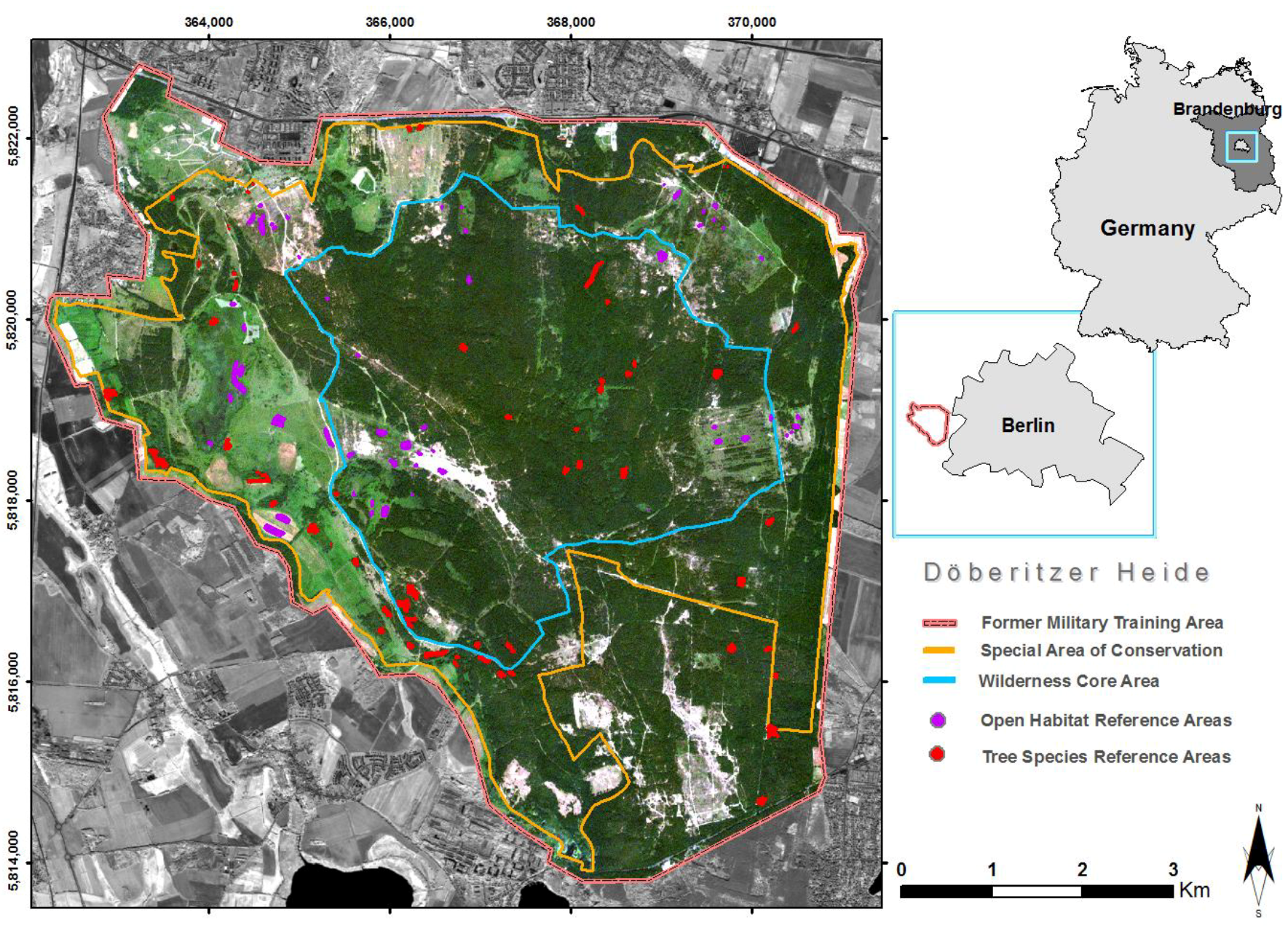
This study was carried out in 2016 and 2017 at the reserve Doeberitzer Heide close to Berlin (52°30′43.7″ N, 13°01′43.5″ E, Figure 1). The reserve is influenced by a temperate seasonal climate with clearly marked cold and warm seasons. Until 1991, the area was in military use. Nowadays, it is a nature reserve and also part of the network “Natura 2000”. The Heinz Sielmann foundation established a fenced core area of about 1860 ha in the middle of the nature reserve in 2010. In 2010 and 2011, the first European bison and Przewalski’s horses were introduced to this core area. For the horses, six mares and sixteen geldings (castrated males) were introduced (n = 22). The age ranged from six- to eighteen-year-old individuals. Concerning the bison in the area (n = 80), the gender ratio was nearly equable and the age ranged from newborn calves to ten-year-old individuals. The fenced area comprised different habitat types like deciduous forest, pine forest, meadow, wet sedge meadow, and dry grassland. Five solar-powered waterers provided water. There was no human intervention such as supplementary feeding.
2.2. Diet Selection
Direct observation was used to study diet selection of European bison and Przewalski’s horses. Over a period of one year, each species was observed for two days every week. Either bison or horses were observed, not both species at the same time. Observations were made from dawn to dusk. Thus, the length of observations differed among seasons, but did not differ between species. Animals were found while driving on the few tracks through the reserve. For the horses, all 22 individuals were observed over the whole study period. The approximately 80 bison of both sexes did not have constant herds. Therefore, various groups as well as single individuals were observed over the year. Over all, approximately 50 different bison individuals were monitored. All observation procedures followed accepted methods [33] respecting animal welfare. Disturbances were minimized by staying approximately 50–100 m away from the animals while sitting in a car and using binoculars. Even in forest habitats, this was possible because of the open forest character. After observation of bison or horses, marks of grazing on plant species were visually checked. The type of habitat and selected bitten plants were noted for every observation. The year was divided into four seasons: spring (March, April, May), summer (June, July, August), autumn (September, October, November), and winter (December, January, February). All plant species were classified into groups from 3 (always selected) to 1 (rarely selected), which reflect the preferences. Subsequently, a fourth category was created for plant species that were selected by one of the animal species, but not by the other—they were categorized in group 0 (rejected) for the latter (Table 1).
2.3. Satellite Imagery
The spectral radiance reflected from the Earth’s surface was recorded in five spectral bands within the wavelength range of visible/red-edge/near-infrared (440–850 nm) using the RapidEye five-satellite constellation. Multispectral satellite imageries were provided via the Planet Labs, Inc. archive for the years 2014–2016. In every year, only scenes exhibiting 100% cloud free pixels were selected over a whole phenological vegetation period. Whereas in 2014 and 2015, four scenes could be recorded (2014: 09.03./28.04./06.08./04.09. and 2015: 18.03./04.07./03.08./12.10), the year 2016 held five cloud free scenes (04.03./01.04./05.05./24.06./10.09.), resulting in 65 wavebands for the final time-stack. Subsequently, the recorded sensor radiance values were atmospherically corrected using Atmospheric & Topographic Correction for Satellite Images ATCOR [53] in order to calculate surface reflectance values for every scene individually. Geometric correction was performed at Planet Labs, Inc., followed by an in-house co-registration procedure to geometrically align all scenes towards one master image with a final spatial resolution of 5 m [54].
2.4. Habitat Categorization
For habitat classification, we used remote sensing and machine learning techniques [50,51,52] in combination with ground truthing, similar to Neumann et al. [55,56]. Habitat units were defined a priori according to the number of known tree species that form dominance stands with an area of at least three RapidEye pixels (i.e., 15 m by 15 m) and general habitat categories that were based on preliminary field work and experiences from vegetation level classification [57]. In particular, the open habitat categories were defined in accordance with the plant community concept, grouping together plant associations for distinct ecological niches [58,59]. The study area comprises interpenetrating numbers of niches that are mainly established along moisture and nutrient gradients such as fresh meadows, wet meadows, or xeric grasslands and calcareous grasslands. In the case of the current study, the final habitat classification was not strictly based on niche inventories, but was performed according to years of field experience in order to cover the complete natural variability of the underlying ecological gradients. As a result, the study area was categorized into 12 areas determined by tree species and 14 openland habitat categories. Field surveys were conducted during the summer seasons of 2015 and 2016, when polygon areas of 77 homogeneous tree species stands and 57 openland habitat areas were mapped in situ. Owing to the degree of connectivity of homogeneous habitat patches, the number of pixels varied between habitat categories. For model calibration, the pixels under mapped polygon areas were extracted for each RapidEye scene on the basis of polygon coordinates. Hence, each single pixel represents a spectral time-stack for the related polygon habitat category. In total, 7310 pixels could be allocated as forest habitats and 4257 pixels were defined as openland habitats that together form the basis for model calibration (Figure 1).
2.5. Spectral Habitat Modeling
The study uses a random forest [60,61] classification approach, which is a frequently used machine learning technique for remote sensing image interpretation [52,62,63]. Thereby, n = 500 decision trees were generated randomly using m < predictor variables (spectral reflectance bands) at each splitting node. Image data handling was realized using the package raster 2.6 [64] and classification was performed with package random Forest 4.6 [65]. For statistical analyses and visualization, we used the programming language R v. 3.4.2 [66].Every single decision tree votes for a habitat membership of image pixels from a bootstrapped calibration dataset. Bootstrapping was applied on the initial reference polygon pixels, whereby habitats were modeled (a) altogether in order to distinguish between forest and open habitats and (b) separately for openland and forest polygons for fine-scale delineation of habitat gradients and tree species; thus, three independent models were finally calibrated. Therein, the final habitat membership was defined using a class majority vote over all trees within the individual classification models. Validation was performed internally by testing the remaining ~30% bootstrapped excluded pixels that were not used for calibration. A confusion matrix was calculated to show the statistical error metrics for class reliabilities based on out-of-bag error estimates as a direct outcome for the pixels that were not used in all single tree calibrations. The first model was then applied on the whole time-stack to separate forest from openland habitats. Finally, the remaining two models were applied only in their respective habitat unit to map a spatially explicit distribution of fine-scale habitat categories and tree species.
2.6. Mapping of Potential Habitat Preferences
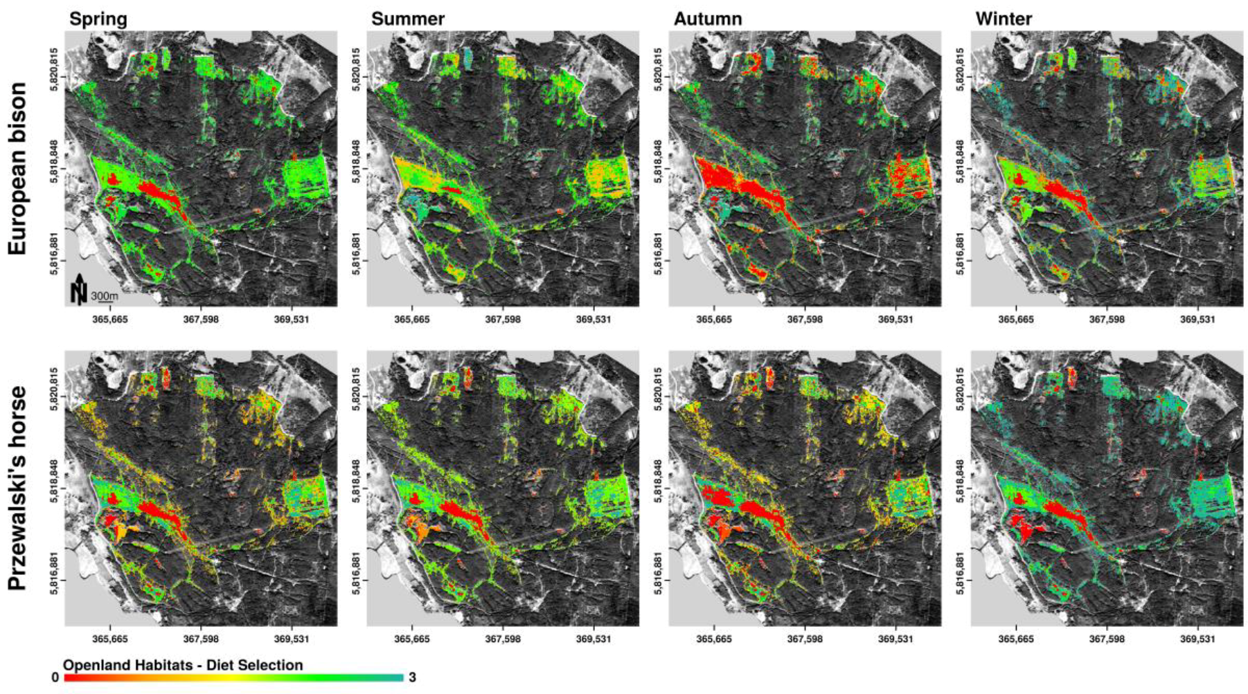
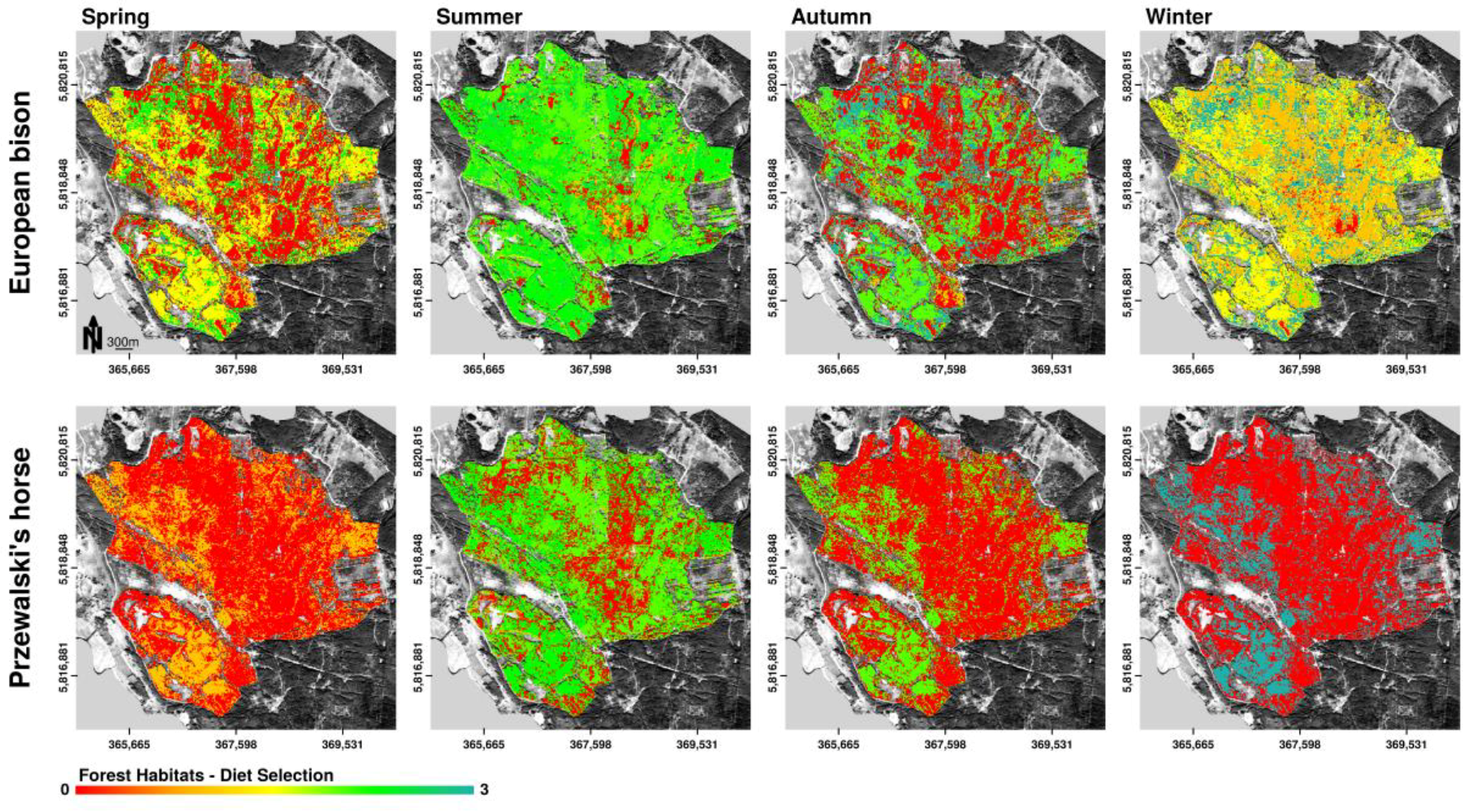
Selected fodder plants were assigned to the different determined habitats according to their occurrence (Table S1). In order to spatially map the potential habitat preferences based on the distribution of selected forage in the study area, the selected plant species were grouped concerning their preference (0–3, see above) and averaged for the observation periods of spring, summer, autumn, and winter for bison and horse separately. Determined habitats may contain several fodder plants with different preferences. Therefore, mapped potential habitat preferences can be built up by various forage preference categories. This results in a continuous scale of habitat preferences. Equal use of the same habitat type irrespective of its position in the study area or distance to water or fences is assumed. Each habitat category, or tree species, respectively, was then related to the potential habitat preference and plotted for the entire study area.
2.7. Diet Data Analyses
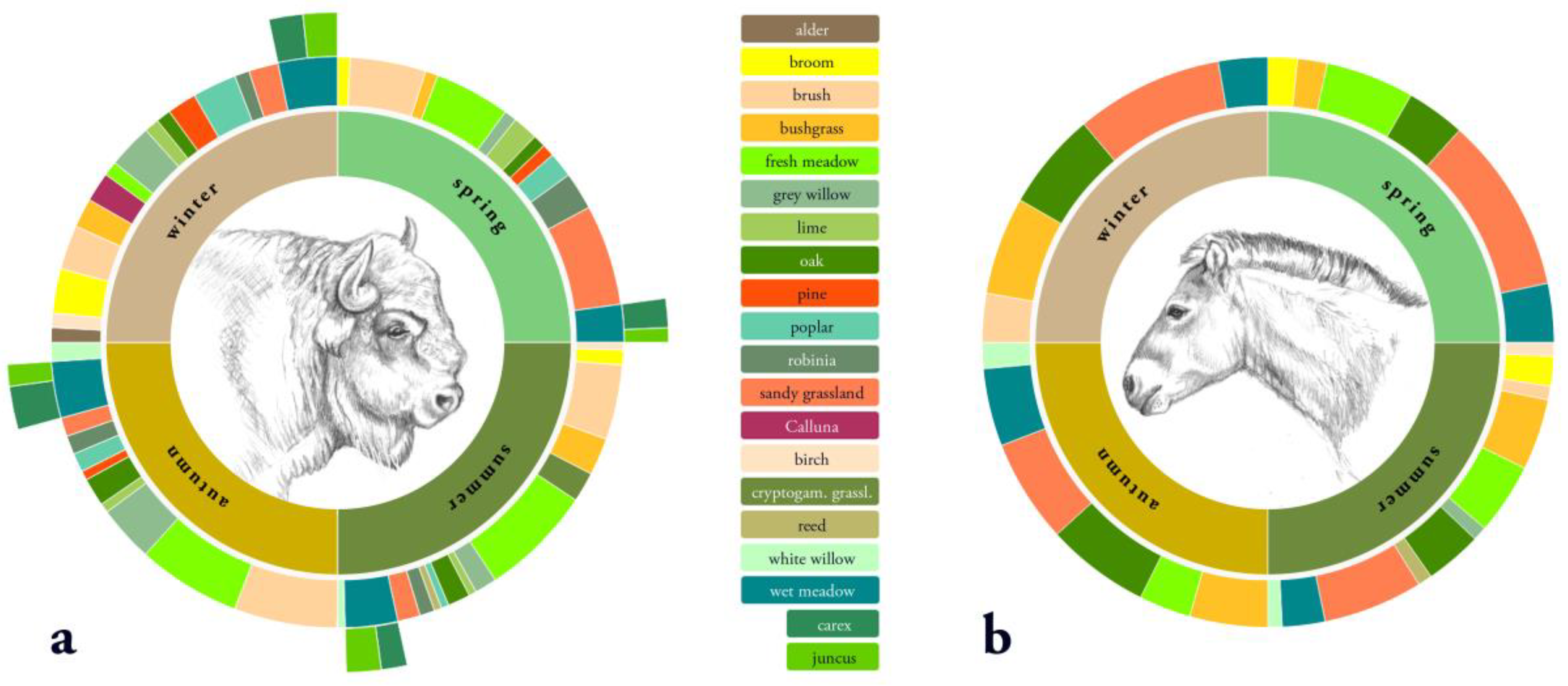
Two-way contingency tables were applied to analyze abundance frequencies of the habitat-inherent fodder sources within habitat and seasons for European bison and Przewalski’s horse separately. Chi-square-test after Pearson was used to examine dependencies of the frequencies of observed fodder plants in the survey collections on the factors ‘habitat’ and ‘season’. After adjusting for every season, percentages of the preferred habitat corresponding plants were arranged as sunburst plots with the season as the core factor and the habitat as the outer ring for both animals. All analyses were done using scripts written in the statistical computing environment of R [66].
3. Results
3.1. Habitat Classification
The averaged overall accuracy (OAA) over all n = 500 decision trees in model validation was high, with an OAA = 99.79% for tree species classification and OAA = 99.81% for openland habitats. Almost all pixels could be allocated to their defined class in both classification forests using excluded bootstrapped samples. Table 2 and Table 3 show the specific user’s and producer’s accuracy along all pixels of defined habitat units. Owing to the exclusive selection of habitats that occurred in connected homogeneous patches (tree species patches) for habitat categorization, the classes white willow, ash leaf maple, open sand, and water exhibited only a small number of pixels for calibration. The low abundance of pure pixel findings for these classes reduced the amount of available calibration data in the study area. However, both accuracy measures were high (>90%) over all classes, with slight misclassification, mainly between heath and pine, between downy birch and birch, and between open sand and cryptogams pixels. These class pairs show similar reflectance characteristics (needle-like leafs, similar species, or sand cryptogams interpenetration) that cannot be resolved significantly in 5 m spatial pixel resolution. Pine habitats can be found in both classification models because the first model designated needle tree areas to the openland category within the first classification step.
3.2. Habitat Distribution within the Study Area
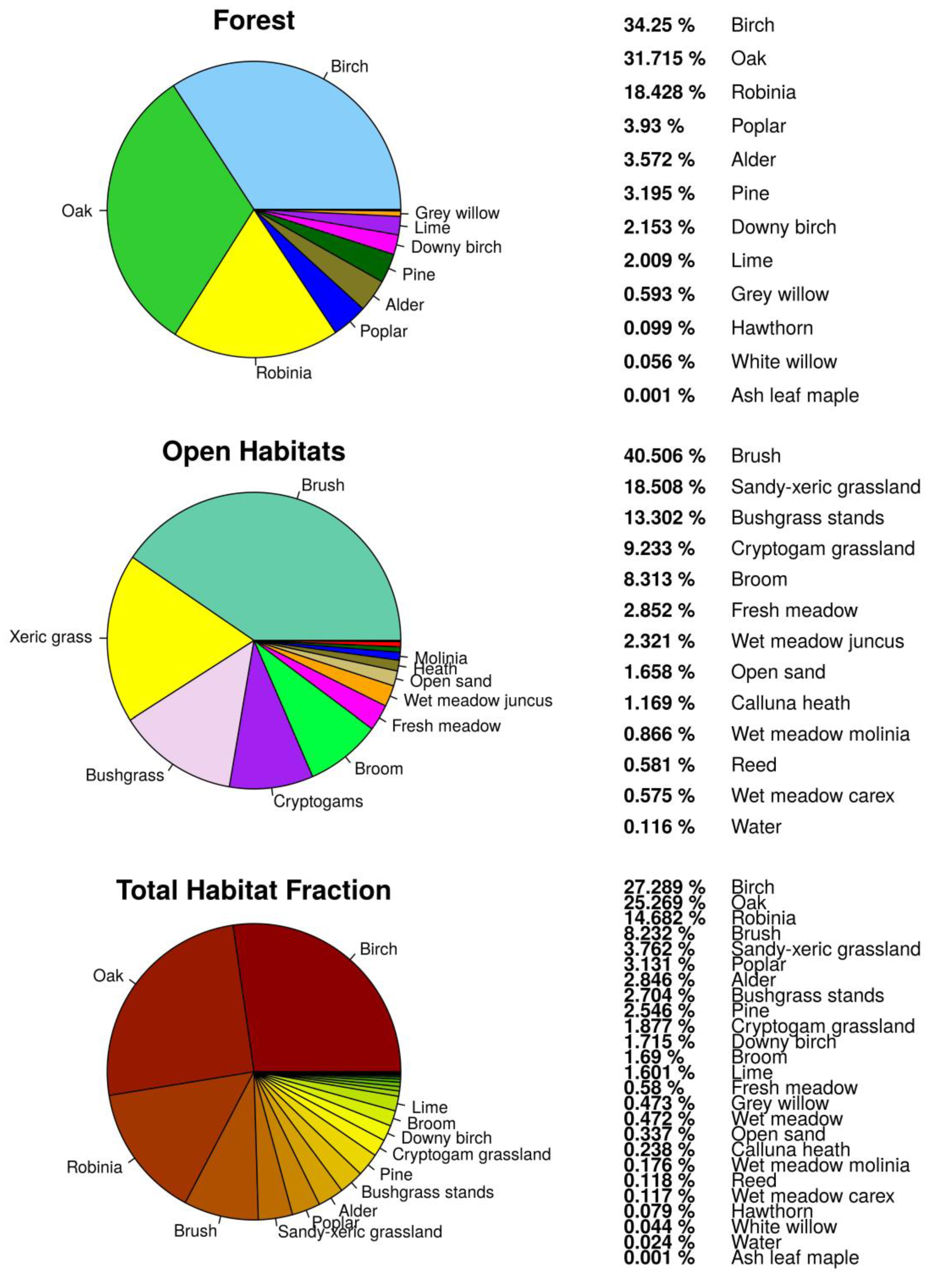
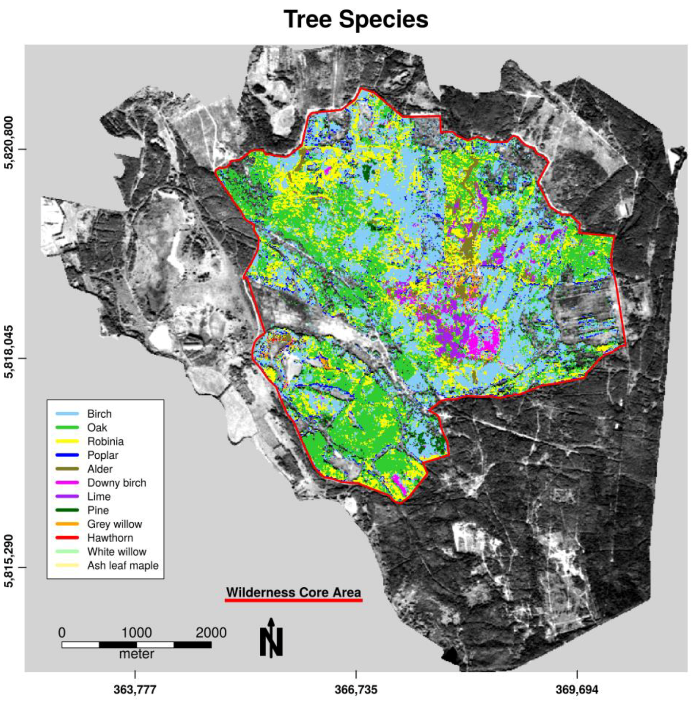
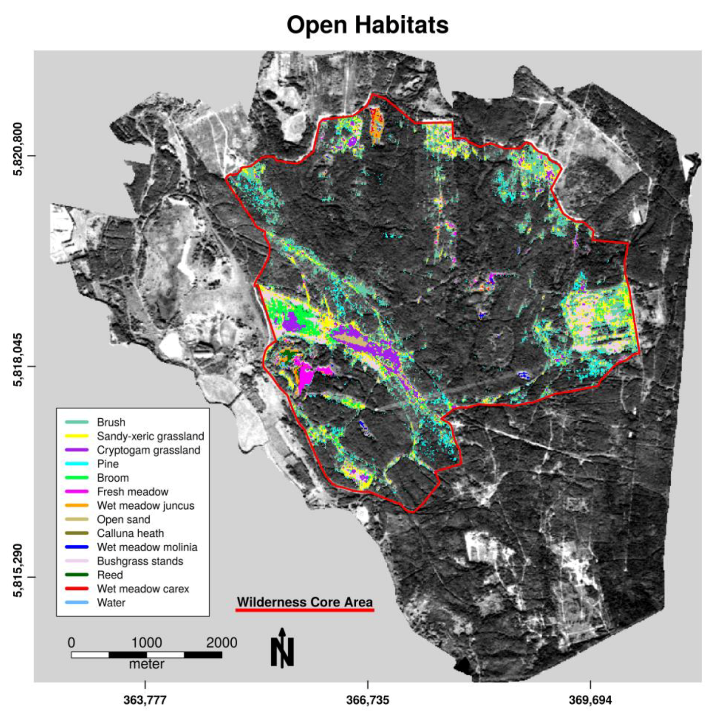
As presented in Figure 2, 79.7% of the study area was covered by forest habitats and 20.3% by openland habitats. Water as part of openland habitats had a total cover of less than 1%. Forest was the most abundant vegetation class in the study area and was mainly formed by twelve tree species (Figure 3). Deciduous and mixed tree stands consisted mainly of birch (Betula pendula 34.2%), oak (Quercus robur 31.7%), black locust (Robinia pseudoacacia 18.4%), poplar (Populus tremula 3.9%), alder (Alnus glutinosa 3.5%), and pine (Pinus silvestris 3.2%) (Figure 3). Openland habitats were classified into fourteen habitat types of different size and mainly found close to the fence (Figure 4). Openland habitats were made up mostly by brush (40.5%), sandy–xeric grassland (18.5%), bushgrass stands (13.3%), and cryptogam grassland (9.3%) (Figure 2). Wet openland habitats dominated by sedges and rushes were rare (wet meadow Carex 0.58%, wet meadow Juncus 2.32%).
3.3. Diet Selection
The pattern of bitten plants was significantly influenced by season and habitat for both European bison (χ² (279) = 818.1, p < 0.001) and Przewalski’s horses (χ² (279) = 703.8, p < 0.001). European bison and Przewalski’s horses showed intra-annual differences in forage preference (Figure 5). Whereas bison included a high number of different forage plants in their diet, horses tended to prefer almost the same forage plants year round. European bison had a much higher proportion of woody material in their diet. For both European bison and Przewalski’s horses, debarking mostly occurred in winter and spring, with almost no debarking in summer. European bison used foliage and bark from different tree species, whereas Przewalski’s horses predominantly showed preferences for foliage (spring and summer) and bark of oak (winter). The diet composition of the observed European bison was more diverse than that of the Przewalski’s horses during the study period. This resulted in a different habitat use for food selection throughout most of the year for both species. European bison showed a high variation in the use of different habitat types for foraging. However, Przewalski’s horses used nearly the same habitat types in all seasons.
3.3.1. Diet Selection Openland Habitats
On the basis of the distribution of selected forage plants in the study area, European bison as well as Przewalski’s horses showed seasonal changes of trends in openland habitat preferences (Figure 6). Horses preferred openland habitats throughout the year, while bison showed high preferences for openland habitats in spring only. In summer and winter, bison selected forage in openland and forest habitats equally. In autumn, bison rarely selected openland habitats for browsing. The fresh and wet meadows, which together covered less than 1.2% of the total core area, were highly preferred by European bison for food intake in all seasons, but only slightly used by horses. Horses rather selected dry grasslands, especially the habitat types sandy–xeric grassland, as well as bushgrass stands dominated by Calamagrostis epigejos throughout the year. In contrast, bison used plant species in sandy–xeric grasslands only in winter and spring. Bushgrass stands were used rarely. Both horses and bison avoided cryptogam grassland in all seasons. Bison, but not horses additionally showed high preferences for brush in winter and spring.
3.3.2. Diet Selection Forest Habitats
Seasonal changes in forage preferences by European bison as well as Przewalski’s horses led to seasonally changing trends in forest habitat preferences (Figure 7). In summer, autumn, and winter, bison showed high preferences for forage in forest habitats. Overlap in forest habitat use for food intake between bison and horses occurred in summer and slightly in autumn. Both bison and horses showed high preferences for oak (foliage and bark). Additionally, bison, but not horses showed high preferences for forest habitats dominated by black locust (foliage and bark). Both species avoided forest habitats dominated by birch year round.
4. Discussion
This study provides empirical data concerning the selection of fodder plants as well as potential preferences in habitat use by European bison and Przewalski’s horses living under similar conditions in a rewilding area. European bison showed seasonal changes in trends of diet selection. In contrast, Przewalski’s horses showed strong selection for grasses year-round, supplemented with sedges and herbs and some woody material in winter. Przewalski’s horses selected forage plants in open habitats throughout the year, while European bison used open habitats and additionally forest habitats in all seasons.
Horses are generally known as monocotyledon specialists [67,68,69,70,71,72,73,74] and inhabit a wide range of different open habitat types [2,15,75,76,77,78]. In our study, Przewalski’s horses were foraging more on grasses than on browse during all seasons. Therefore, they would be categorized as grazers, similar to the classification of Hofmann [79]. Their strong preference for dry grasslands is probably because of the evolutionary history of E. ferus in Eurasian steppes [80]. The results of our study are comparable to those of Feranec et al. [73], where horses did not show seasonal variation in diet preferences either. The use of bark by equids occurs rarely and not to the extent that European bison are debarking [33]. In our study, we observed some use of oak bark by horses, but only in winter.
European bison preferred fresh and wet meadows with sedges and rushes as key forage species, in association with herbs and grasses during spring, summer, and autumn. Additionally, they moved into forest habitats to forage on foliage, especially on leaves of oak. On the basis of the distribution of preferred forage plants, European bison are expected to prefer openland habitats in spring. Then, most forage plants are of high quality owing to low fibre content and high digestibility [81,82,83].
During autumn, European bison started to broaden their diet. This led to the potential use of a wide range of habitats within the study area. During winter, the diet of European bison was dominated by woody material and they predominantly used forested habitats. The use of woody material and debarking in winter by European bison is a well-known phenomenon [14,33,84]. A larger consumption of woody shrubs in autumn when graminoids are scarce was also observed for American bison (Bison bison) in a study by Bergmann et al. [35]. Both Waggoner and Hinkes [85] and Larter and Gates [86] reported an increased use of shrubs by American bison and Wood bison (Bison bison athabascae) due to limited availability of sedges and rushes in winter. Traditionally, the habitat for European bison is considered to be forest because the last wild living individuals inhabited forests [14,87]. However, several recently published studies agree that European bison tend to use open habitats preferentially [24,33,79,84,88,89,90,91].
The increasing use of woody material in autumn and winter by the observed European bison could be a result of limited availability of other suitable fodder. Preferred plants might have already been heavily grazed in the study area as habitats containing preferred forage cover less than 1.2% of the total core area (fresh and wet meadows). Animals were thus forced to use different forages. Additionally, there were more bison than horses in the study area and the grazing pressure in preferred habitats was higher. The intense selection of woody material by European bison might be an indication for inappropriate habitats in general.
Przewalski’s horses and European bison used the available fodder resources in the study area differently. European bison are, like cattle, unable to feed on very short grasses. Therefore, European bison are more constrained by plant height, but less constrained by secondary metabolites compared with Przewalski’s horses; cattle as well as European bison are able to better digest plants with secondary metabolites than horses [23,92]. Horses are able to extract more nutrients than bovids from grasses with a high fibre content [93,94,95]. Additionally, horses are able to feed on grass too close to the ground for bovids [23,96] and are thus able to forage in heavily grazed habitats. In the study area, European bison and Przewalski’s horses differed in their feeding niches throughout most of the year. Overlap only occurred in the cold season when available forage was scarce and in spring when the first shoots started to grow. Even the use of the same habitats does not necessarily lead to food competition because different forage plants can be preferred.
The phenomenon of resource partitioning among large herbivores has been reported for palaeoecosystems as well as modern ecosystems [33,73,97,98,99]. Through resource partitioning, different digestive systems, and diverse foraging strategies, species can coexist within ecosystems [92,100,101]. The illustrated potential habitat preferences of European bison and Przewalski’s horses according to the distribution of selected food plants in the different habitat types assumes an equal use of each habitat within the study area. However, other factors like snow depth in winter, risk of disturbance, or the availability of water can have additional influences on preferred habitat types and the distribution of animals across the landscape [102,103,104,105,106,107,108]. Thus, the distance to waterers or the distance to fences might additionally influence the use of habitats by the animals in the Doeberitzer Heide. This needs to be tested in future studies, for example, by the use of animal tracking techniques such as Global Positioning System (GPS) collars [109,110,111]. Additionally, fecal DNA metabarcoding could be used to further expand the knowledge on animals’ diets [112]. Further long-term studies are needed to determine the extent of inter-annual differences in forage availability and use.
European bison and Przewalski’s horses differed in their diet selection and did not generally compete with each other over the study period. We showed that resource partitioning between European bison and Przewalski’s horses occurred by their selection of diets in different habitats. Thus, these two species were not in direct competition for resources throughout most of the year.
5. Conclusions
In the context of nature conservation management and rewilding projects, European bison and Przewalski’s horses could represent one possibility to maintain open land and grassland habitats with limited management effort. European bison and Przewalski’s horses have the potential for co-existence in a heterogeneous area. Comparative foraging and feeding niches should be considered in the establishment of multispecies projects to maximize the outcome of restoration processes. European bison might need more open habitat, especially fresh and wet meadows, than so far assumed.
Supplementary Materials
The following are available online at https://www.mdpi.com/1424-2818/11/4/63/s1. Table S1: List of preferred plant species eaten by both European bison and Przewalski’s horses from June 2016 until March 2017 and the allocation to the determined habitat types within the study area Doeberitzer Heide.
Author Contributions
Conceptualization, L.Z., N.W.-M., J.M., and C.N; Methodology, L.Z., N.W.-M., J.M., and C.N.; Project administration, N.W.-M.; Data collection, L.Z; Visualization, J.M and C.N; Supervision, N.W.-M. and J.M.; Writing—original draft, L.Z., J.M., and C.N; Writing—review & editing, L.Z., N.W.-M., J.M., and C.N.
Funding
This research received no external funding.
Acknowledgments
We thank the Heinz Sielmann Foundation for the cooperation and the access to the reserve.
Conflicts of Interest
The authors declare no conflict of interest.
References
- Aaris-Sørensen, K.; Mühldorff, R.; Petersen, E.B. The Scandinavian reindeer (Rangifer tarandus L.) after the last glacial maximum: Time, seasonality and human exploitation. J. Archaeol. Sci. 2007, 34, 914–923. [Google Scholar]
- Sommer, R.S.; Benecke, N.; Lõugas, L.; Nelle, O.; Schmölcke, U. Holocene survival of the wild horse in Europe: A matter of open landscape? J. Quat. Sci. 2011, 26, 805–812. [Google Scholar] [CrossRef]
- Svenning, J.C. A review of natural vegetation openness in north-western Europe. Biol. Conserv. 2002, 104, 133–148. [Google Scholar] [CrossRef]
- Gordon, I.J.; Hester, A.J.; Festa-Bianchet, M. The management of wild large herbivores to meet economic, conservation and environmental objectives. J. Appl. Ecol. 2004, 41, 1021–1031. [Google Scholar] [CrossRef]
- Kuijper, D.P.J.; Cromsigt, J.P.M.G.; Churski, M.; Adams, B.; Jedrzejewska, B.; Jedrzejewski, W. Do ungulates preferentially feed in forest gaps in European temperate forests? For. Ecol. Manag. 2009, 258, 1528–1535. [Google Scholar] [CrossRef]
- Griffiths, C.; Harris, S. Prevention of Secondary Extinctions through Taxon Substitution. Conserv. Biol. 2010, 24, 645–646. [Google Scholar] [CrossRef] [PubMed]
- Svenning, J.C.; Pedersen, P.B.M.; Donlan, C.J.; Ejrnӕs, R.; Faurby, S.; Galetti, M.; Hansen, D.M.; Sandel, B.; Sandom, C.J.; Terborgh, J.W.; et al. Science for a wilder Anthropocene: Synthesis and future directions for trophic rewilding research. Proc. Natl. Acad. Sci. USA 2016, 113, 898–906. [Google Scholar] [CrossRef]
- Owen-Smith, R.N. Megaherbivores: The Influence of Very Large Body Size on Ecology; Cambridge University Press: Cambridge, UK, 1988. [Google Scholar]
- Olff, H.; Ritchie, M.E. Effects of herbivores on grassland plant diversity. Tree 1998, 13, 261–265. [Google Scholar] [CrossRef]
- Beever, E.A.; Tausch, R.J.; Thogmartin, W.E. Multi-scale responses of vegetation to removal of horse grazing from Great Basin (USA) mountain ranges. Plant Ecol. 2008, 196, 163–184. [Google Scholar] [CrossRef]
- Estes, J.A.; Terborgh, J.; Brashares, J.S.; Power, M.E.; Berger, J.; Bond, W.J.; Carpenter, S.R.; Essington, T.S.; Holt, R.D.; Jackson, J.B.C.; et al. Trophic downgrading of planet Earth. Science 2011, 333, 301–306. [Google Scholar] [CrossRef] [PubMed]
- Schwark, L.; Zink, K.; Lechterbeck, J. Reconstruction of postglacial to early Holocene vegetation history in terrestrial central Europe via cuticular lipid biomarkers and pollen records from lake sediments. Geology 2002, 30, 463–466. [Google Scholar] [CrossRef]
- Birks, H.J.B. Mind the gap: How open were European primeval forests? Trends Ecol. Evol. 2005, 20, 154–156. [Google Scholar] [CrossRef]
- Kowalczyk, R.; Taberlet, P.; Coissac, E.; Valentini, A.; Miquel, C.; Kaminski, T.; Wojcik, J.M. Influence of management practices on large herbivore diet-Case of European bison in Białowieża Primeval Forest (Poland). For. Ecol. Manag. 2011, 261, 821–828. [Google Scholar] [CrossRef]
- Naundrup, P.J.; Svenning, J.C. A Geographic Assessment of the Global Scope for Rewilding with Wild-Living Horses (Equus ferus). PLoS ONE 2015, 10, e0132359. [Google Scholar] [CrossRef] [PubMed]
- Soule, M.; Noss, R. Rewilding and biodiversity: Complementary goals for continental conservation. Wild Earth 1998, 8, 1–11. [Google Scholar]
- Schumacher, H.; Finck, P.; Klein, M.; Ssymank, A.; Paulsch, C. Wildnis im Dialog—Wildnis und Natura 2000; BfN-Skripten 452; Bundesamt für NaturschutzKonstantinstr: Bonn, Germany, 2017; p. 126. [Google Scholar]
- Danell, K.; Bergström, R.; Duncan, P.; Pastor, J. Large Herbivore Ecology, Ecosystem Dynamics and Conservation; Cambridge University Press: Cambridge, UK, 2006. [Google Scholar]
- Waldram, M.S.; Bond, W.J.; Stock, W.D. Ecological engineering by a mega-grazer: White rhino impacts on a South African savanna. Ecosystems 2008, 11, 101–112. [Google Scholar] [CrossRef]
- Haynes, G. Elephants (and extinct relatives) as earth-movers and ecosystem engineers. Geomorphology 2012, 157–158, 99–107. [Google Scholar] [CrossRef]
- Jaroszewicz, B.; Pirożnikow, E. Diversity of plant species eaten and dispersed by the European bison Bison bonasus in the Białowieża Forest. Eur. Bison Conserv. Newsl. 2008, 1, 14–29. [Google Scholar]
- Finck, P.; Riecken, U.; Schröder, E. Pasture Landscapes and Nature Conservation—New strategies for the preservation of open landscapes in Europe. In Pasture Landscapes and Nature Conservation; Springer: Berlin/Heidelberg, Germany, 2002; pp. 1–13. [Google Scholar]
- Menard, C.; Duncan, P.; Fleurance, G.; Georges, J.Y.; Lila, M. Comparative foraging and nutrition of horses and cattle in European wetlands. J. Appl. Ecol. 2002, 39, 120–133. [Google Scholar] [CrossRef]
- Kerley, G.I.H.; Kowalczyk, R.; Cromsigt, J.P.G.M. Conservation implications of the refugee species concept and the European bison: King of the forest or refugee in a marginal habitat? Ecography 2011, 35, 519–529. [Google Scholar] [CrossRef]
- Smit, C.; Ruifrok, J.L.; van Klink, R.; Olff, H. Rewilding with large herbivores: The importance of grazing refuges for sapling establishment and wood-pasture formation. Biol. Conserv. 2015, 182, 134–142. [Google Scholar] [CrossRef]
- Hofman-Kaminska, E.; Kowalczyk, R. Farm crops depredation by European bison (Bison bonasus) in the vicinity of forest habitats in northeastern Poland. Environ. Manag. 2012, 50, 530–541. [Google Scholar] [CrossRef] [PubMed]
- Van Dierendonck, M.C.; Wallis de Vries, M.F. Ungulate reintroduction: Experiences with the Takhi or Przewalski Horse (Equus ferus przewalskii) in Mongolia. Conserv. Biol. 1996, 10, 728–740. [Google Scholar] [CrossRef]
- Jackson, J. The Red-Cockaded Woodpecker Recovery Program: Professional Obstacles to Co-Operation. In Species Recovery: Finding the Lessons, Improving the Process; Clark, T.W., Reading, R.P., Clarke, A.L., Eds.; Endangered Island Press: Washington, DC, USA, 1994; pp. 157–181. [Google Scholar]
- Boyd, L.; Bandi, N. Reintroduction of takhi, Equus ferus przewalskii, to Hustai National Park, Mongolia: Time budget and synchrony of activity pre- and post release. Appl. Anim. Behav. Sci. 2002, 78, 87–102. [Google Scholar] [CrossRef]
- King, S.R.B. Home range and habitat use of free-ranging Przewalski horses at Hustai National Park, Mongolia. Appl. Anim. Behav. Sci. 2002, 78, 103–113. [Google Scholar] [CrossRef]
- Hughes, F.M.R.; Stroh, P.A.; Adams, W.M.; Kirby, K.J.; Mountford, J.O.; Warrington, S. Monitoring and evaluating large-scale, ′open-ended′ habitat creation projects: A journey rather than a destination. J. Nat. Conserv. 2011, 19, 245–253. [Google Scholar] [CrossRef]
- Ramos, A.; Petit, O.; Longour, P.; Pasquaretta, C.; Sueur, C. Space use and movement patterns in a semi-free-ranging herd of European bison (Bison bonasus). PLoS ONE 2016, 11, e0147404. [Google Scholar] [CrossRef]
- Cromsigt, J.P.G.M.; Kemp, Y.J.M.; Rodriguez, E.; Kivit, H. Rewilding Europe’s large grazer community: How functionally diverse are the diets of European bison, cattle, and horses? Restor. Ecol. 2017, 26, 891–899. [Google Scholar] [CrossRef]
- Deinet, S.; Ieronymidou, C.; McRae, L.; Burfield, I.J.; Foppen, R.P.; Collen, B.; Böhm, M. Wildlife Comeback in Europe: The Recovery of Selected Mammal and Bird Species; Final report to Rewilding Europe by ZSL, BirdLife International and the European Bird Census Council; ZSL: London, UK, 2013. [Google Scholar]
- Bergmann, G.T.; Craine, J.M.; Robeson, M.S., II; Fierer, N. Seasonal Shifts in Diet and Gut Microbiota of the American bison (Bison bison). PLoS ONE 2015, 10, e0142409. [Google Scholar] [CrossRef]
- Corbane, C.; Lang, S.; Pipkins, K.; Alleaume, S.; Deshayes, M.; GarcíaMillán, V.E.; Strasser, T.; Vanden Borre, J.; Toon, S.; Michael, F. Remote sensing for mapping natural habitats and their conservation status—New opportunities and challenges. Int. J. Appl. Earth Obs. 2015, 37, 7–16. [Google Scholar] [CrossRef]
- Gómez, C.; White, J.C.; Wulder, M.A. Optical remotely sensed time series data for land cover classification: A review. ISPRS J. Photogramm. Remote Sens. 2016, 116, 55–72. [Google Scholar] [CrossRef]
- Joshi, N.; Baumann, M.; Ehammer, A.; Fensholt, R.; Grogan, K.; Hostert, P.; Jepsen, M.R.; Kuemmerle, T.; Meyfroidt, P.; Mitchard, E.T.; et al. A review of the application of optical and radar remote sensing data fusion to land use mapping and monitoring. Remote Sens. 2016, 8, 70. [Google Scholar] [CrossRef]
- Turner, W.; Spector, S.; Gardiner, N.; Fladeland, M.; Sterling, E.; Steininger, M. Remote sensing for biodiversity science and conservation. Trends Ecol. Evol. 2003, 18, 306–314. [Google Scholar] [CrossRef]
- Förster, M.; Frick, A.; Walentowski, H.; Kleinschmit, B. Approaches to utilising QuickBird data for the monitoring of NATURA 2000 habitats. Community Ecol. 2008, 9, 155–168. [Google Scholar] [CrossRef]
- Förster, M.; Schmidt, T.; Schuster, C.; Kleinschmit, B. Multi-temporal detection of grassland vegetation with RapidEye imagery and a spectral-temporal library. In Proceedings of the 2012 Geoscience and Remote Sensing Symposium (IGARSS), Munich, Germany, 10 July 2012; pp. 4930–4933. [Google Scholar]
- Schuster, C.; Schmidt, T.; Conrad, C.; Kleinschmit, B.; Förster, M. Grassland habitat mapping by intra-annual time series analysis–Comparison of RapidEye and TerraSAR-X satellite data. Int. J. Appl. Earth Obs. 2015, 34, 25–34. [Google Scholar] [CrossRef]
- Laliberte, A.S.; Rango, A.; Havstad, K.M.; Paris, J.F.; Beck, R.F.; McNeely, R.; Gonzalez, A.L. Object-oriented image analysis for mapping shrub encroachment from 1937 to 2003 in southern New Mexico. Remote Sens Environ. 2004, 93, 198–210. [Google Scholar] [CrossRef]
- Selkowitz, D.J. A comparison of multi-spectral, multi-angular, and multi-temporal remote sensing datasets for fractional shrub canopy mapping in Arctic Alaska. Remote Sens Environ. 2010, 114, 1338–1352. [Google Scholar] [CrossRef]
- Coppin, P.R.; Bauer, M.E. Digital change detection in forest ecosystems with remote sensing imagery. Remote Sens. Rev. 1996, 13, 207–234. [Google Scholar] [CrossRef]
- Key, T.; Warner, T.A.; McGraw, J.B.; Fajvan, M.A. A comparison of multispectral and multitemporal information in high spatial resolution imagery for classification of individual tree species in a temperate hardwood forest. Remote Sens. Environ. 2001, 75, 100–112. [Google Scholar] [CrossRef]
- Kim, M.; Madden, M.; Warner, T.A. Forest type mapping using object-specific texture measures from multispectral Ikonos imagery. Photogramm. Eng. Remote Sens. 2009, 75, 819–829. [Google Scholar] [CrossRef]
- Feilhauer, H.; Thonfeld, F.; Faude, U.; He, K.S.; Rocchini, D.; Schmidtlein, S. Assessing floristic composition with multispectral sensors—A comparison based on monotemporal and multiseasonal field spectra. Int. J. Appl. Earth Obs. 2013, 21, 218–229. [Google Scholar] [CrossRef]
- Feilhauer, H.; Dahlke, C.; Doktor, D.; Lausch, A.; Schmidtlein, S.; Schulz, G.; Stenzel, S. Mapping the local variability of Natura 2000 habitats with remote sensing. Appl. Veg. Sci. 2014, 17, 765–779. [Google Scholar] [CrossRef]
- Kampichler, C.; Wieland, R.; Calmé, S.; Weissenberger, H.; Arriaga-Weiss, S. Classification in conservation biology: A comparison of five machine-learning methods. Ecol. Inf. 2010, 5, 441–450. [Google Scholar] [CrossRef]
- Mountrakis, G.; Im, J.; Ogole, C. Support vector machines in remote sensing: A review. ISPRS J. Photogramm. Remote Sens. 2011, 66, 247–259. [Google Scholar] [CrossRef]
- Belgiu, M.; Drăguţ, L. Random forest in remote sensing: A review of applications and future directions. ISPRS J. Photogramm. Remote Sens. 2016, 114, 24–31. [Google Scholar] [CrossRef]
- Richter, R.; Schläpfer, D. Atmospheric/Topographic Correction for Satellite Imagery; ATCOR-2/3 User Guide, Version 8.3. 1, February 2014; DLR-German Aerospace Center: Wessling, Germany; ReSe Appl. Schläpfer Langeggweg 3: Wil, Switzerland, 2013. [Google Scholar]
- Scheffler, D.; Hollstein, A.; Diedrich, H.; Segl, K.; Hostert, P. AROSICS: An automated and robust open-source image co-registration software for multi-sensor satellite data. Remote Sens. 2017, 9, 676. [Google Scholar] [CrossRef]
- Neumann, C.; Weiss, G.; Schmidtlein, S.; Itzerott, S.; Lausch, A.; Doktor, D.; Brell, M. Gradient-Based Assessment of Habitat Quality for Spectral Ecosystem Monitoring. Remote Sens. 2015, 7, 2871–2898. [Google Scholar] [CrossRef]
- Neumann, C.; Itzerott, S.; Weiss, G.; Kleinschmit, B.; Schmidtlein, S. Mapping multiple plant species abundance patterns—A multiobjective optimization procedure for combining reflectance spectroscopy and species ordination. Ecol. Inf. 2016, 36, 61–76. [Google Scholar] [CrossRef]
- Neumann, C.; Weiss, G.; Itzerott, S.; Kuehling, M.; Fuerstenow, J.; Luft, L.; Nitschke, P. Entwicklung und Erprobung eines innovativen, naturschutzfachlichen Monitoringverfahrens auf der Basis von Fernerkundungsdaten am Beispiel der Doeberitzer Heide, Brandenburg; GFZ German Research Centre: Potsdam, Germany, 2013. [Google Scholar]
- Clements, F.E. Plant Succession: An Analysis of the Development of Vegetation; Carnegie Institution of Washington: Washington, DC, USA, 1916. [Google Scholar]
- Whittaker, R.H. Classification of natural communities. Bot. Rev. 1962, 28, 1–239. [Google Scholar] [CrossRef]
- Breiman, L. Random forests. Mach. Learn. 2001, 45, 5–32. [Google Scholar] [CrossRef]
- Cutler, D.R.; Edwards, T.C.; Beard, K.H.; Cutler, A.; Hess, K.T.; Gibson, J.; Lawler, J.J. Random forests for classification in ecology. Ecology 2007, 88, 2783–2792. [Google Scholar] [CrossRef]
- Lawrence, R.L.; Wood, S.D.; Sheley, R.L. Mapping invasive plants using hyperspectral imagery and Breiman Cutler classifications (Random Forest). Remote Sens. Environ. 2006, 100, 356–362. [Google Scholar] [CrossRef]
- Immitzer, M.; Atzberger, C.; Koukal, T. Tree species classification with random forest using very high spatial resolution 8-band WorldView-2 satellite data. Remote Sens. 2012, 4, 2661–2693. [Google Scholar] [CrossRef]
- Hijmans, R.J. Raster: Geographic Data Analysis and Modeling, R package version 2.6-7; R Foundation for Statistical Computing: Vienna, Austria, 2017. [Google Scholar]
- Liaw, A.; Wiener, M. Classification and Regression by random Forest. R News 2002, 2, 18–22. [Google Scholar]
- R Core Team. R: A Language and Environment for Statistical Computing; R Foundation for Statistical Computing: Vienna, Austria, 2017. [Google Scholar]
- Olsen, F.W.; Hansen, R.M. Food relations of wild free-roaming horses to livestock and big game, Red Desert, Wyoming. J. Range Manag. 1977, 30, 17–20. [Google Scholar] [CrossRef]
- Krysl, L.J.; Hubbert, M.E.; Sowell, B.E.; Plumb, G.E.; Jewett, T.K.; Smith, M.A.; Waggoner, J.W. Horses and cattle grazing in the Wyoming Red Desert. I. Food habits and dietary overlap. J. Range Manag. 1984, 37, 72–76. [Google Scholar] [CrossRef]
- Berger, J. Wild Horses at the Great Basin; University of Chicago Press: Chicago, IL, USA, 1986. [Google Scholar]
- Hunt, W.F.; Hay, R.J.M.; Clark, D. Pasture species preferences by horses in New Zealand. In Proceedings of the XVI International Grassland Congress, Nice, France, 4–11 October 1989; p. 797. [Google Scholar]
- Kissell, R.J., Jr. Competitive Interactions among Bighorn Sheep, Feral Horses, and Mule Deer in Bighorn Canyon National Recreation Area and the Pryor Mountain Wild Horse Range. PhD Thesis, Montana State University, Bozeman, MT, USA, 1996. [Google Scholar]
- Fahnestock, J.T.; Detling, J.K. The influence of herbivory on plant cover and species composition in the Pryor Mountain Wild Horse Range, USA. Plant Ecol. 1999, 144, 145–157. [Google Scholar] [CrossRef]
- Feranec, R.S.; Hadly, E.A.; Paytan, A. Stable isotopes reveal seasonal competition for resources between late Pleistocene bison (Bison) and horse (Equus) from Rancho La Brea, southern California. Palaeogeogr. Palaeoecl. 2009, 271, 153–160. [Google Scholar] [CrossRef]
- Scasta, J.D.; Beck, J.L.; Angwin, C.J. Meta-analysis of diet composition and potential conflict of wild horses with livestock and wild ungulates on western rangelands of North America. Rangel. Ecol. Manag. 2016, 69, 310–318. [Google Scholar] [CrossRef]
- Van Dierendonck, M.C.; Bandi, N.; Batdorj, D.; Dugerlham, S.; Munkhtsog, B. Behavioural observations of reintroduced Takhi or Przewalski horses (Equus ferus przewalskii) in Mongolia. Appl. Anim. Behav. Sci. 1996, 50, 95–114. [Google Scholar] [CrossRef]
- Prins, H.H.T. Origins and development of grassland communities in northwestern Europe. In Grazing and Conservation Management; Wallis de Vries, M.F., van de Koppel, J., Eds.; Kluwer Academic Publishers: Dordrecht, The Netherlands, 1998; pp. 55–105. [Google Scholar]
- Moehlman, P.D. Equids: Zebras, Asses and Horses: Status Survey and Conservation Action Plan; IUCN/SCC Equid Specialist Group; IUCN (The World Conservation Union): Gland, Switzerland; Cambridge, UK, 2002. [Google Scholar]
- Dawson, M.; Lane, C.; Saunders, G. Proceedings of the National Feral Horse Management Workshop; Invasive Animals Cooperative Research Centre: Canberra, Australia, 2006. [Google Scholar]
- Hofmann, R.R. Evolutionary steps of ecophysiological adaptation and diversification of ruminants: A comparative view of their digestive system. Oecologia 1989, 45, 443–457. [Google Scholar] [CrossRef] [PubMed]
- Warmuth, V.; Eriksson, A.; Bower, M.A.; Barker, G.; Barrett, E.; Hanks, B.K.; Shuicheng, L.; Lomitashvili, D.; Ochir-Goryaeva, M.; Sizonov, G.V.; et al. Reconstructing the origin and spread of horse domestication in the Eurasian steppe. Proc. Natl. Acad. Sci. USA 2010, 109, 8202–8206. [Google Scholar] [CrossRef] [PubMed]
- Albon, S.D.; Langvatn, R. Plant phenology and the benefits of migration in a temperate ungulate. Oikos 1992, 65, 502–513. [Google Scholar] [CrossRef]
- Villalba, J.J.; Provenza, F.D.; Bryant, J.P. Consequences of the interaction between nutrients and plant secondary metabolites on herbivore selectivity: Benefits or detriments for plants? Oikos 2002, 97, 282–292. [Google Scholar] [CrossRef]
- Villalba, J.J.; Provenza, F.D.; Han, G.; Provenza, D. Experience influences diet mixing by herbivores: Implications for plant biochemical diversity. Oikos 2004, 107, 100–109. [Google Scholar] [CrossRef]
- Krasińska, M.; Krasiński, Z.A. European Bison—The Nature Monograph; Springer: Berlin/Heidelberg, Germany, 2007. [Google Scholar]
- Waggoner, V.; Hinkes, M. Summer and fall browse utilization by an Alaskan bison herd. J. Wildl. Manag. 1986, 50, 322–324. [Google Scholar] [CrossRef]
- Larter, N.C.; Gates, C.C. Diet and habitat selection of wood bison in relation to seasonal changes in forage quantity and quality. Can. J. Zoo 1991, 69, 2677–2685. [Google Scholar] [CrossRef]
- Bocherens, H.; Hofman-Kamińska, E.; Drucker, D.G.; Schmölcke, U.; Kowalczyk, R. European bison as a refugee species? Evidence from isotopic data on early Holocene bison and other large herbivores in northern Europe. PLoS ONE 2015, 10, e0115090. [Google Scholar] [CrossRef]
- Kowalczyk, R. European bison-king of the forest, or meadows and river valleys? In European Bison Conservation in the Białowieża Forest. Threats and Prospects of the Population Development; Kowalczyk, R., et al., Eds.; Mammal Research Institute, Academy of Science: Bialowieza, Poland, 2010; pp. 123–134. [Google Scholar]
- Kuemmerle, T.; Perzanowski, K.; Chaskovskyy, O.; Ostapowicz, K.; Halada, L.; Bashta, A.T.; Kruhlov, I.; Hostert, P.; Waller, D.M.; Radeloff, V.C. European bison habitat in the Carpathian Mountains. Biol. Conserv. 2010, 143, 908–916. [Google Scholar] [CrossRef]
- Cromsigt, J.P.G.M.; Kerley, G.I.H.; Kowalczyk, R. The difficulty of using species distribution modeling for the conservation of refugee species-the example of European bison. Divers. Distrib. 2012, 18, 1253–1257. [Google Scholar] [CrossRef]
- Zielke, L.; Wrage-Mönnig, N.; Müller, J. Seasonal preferences in diet selection of semi-free ranging European bison (Bison bonasus). Eur. Bison Conserv. Newsl. 2017, 10, 61–70. [Google Scholar]
- Bakker, J.; Van Wieren, S.E. The Impact of Grazing on Plant Communities. In Grazing and Conservation Management; Wallis De Vries, M.F., Bakker, J.P., Van Wieren, S.E., Eds.; Kluwer Academic Publishers: Dordrecht, The Netherlands, 1998; pp. 137–184. [Google Scholar]
- Janis, C.M. The evolutionary strategy of the equidae and the origins of rumen and cecal digestion. Evolution 1976, 30, 757–774. [Google Scholar] [CrossRef] [PubMed]
- Duncan, P.; Foose, T.J.; Gordon, I.J.; Gakahu, C.G.; Lloyd, M. Comparative nutrient extraction from forages by grazing bovids and equids: A test of the nutritional model of equid/bovid competition and coexistence. Oecologia 1990, 84, 411–418. [Google Scholar] [CrossRef]
- Duncan, P. Horses and Grasses. The Nutritional Ecology of Equids and Their Impact on the Camargue; Springer: New York, NY, USA, 1992. [Google Scholar]
- Gordon, I.J. Vegetation community selection by ungulates on the Isle of Rhum. II. Vegetation community selection. J. Appl. Ecol. 1989, 26, 53–64. [Google Scholar] [CrossRef]
- Kurtén, B. Pleistocene Mammals of Europe; Weidenfeld & Nicolson: London, UK, 1968. [Google Scholar]
- MacFadden, B.J.; Cerling, T.E. Mammalian herbivore communities, ancient feeding ecology, and carbon isotopes: A 10 million-year sequence from the Neogene of Florida. J. Vertebr. Paleontol. 1996, 16, 103–115. [Google Scholar] [CrossRef]
- Koch, P.L.; Hoppe, K.A.; Webb, S.D. The isotopic ecology of late Pleistocene mammals in North America Part 1. Florida. Chem. Geol. 1998, 152, 119–138. [Google Scholar] [CrossRef]
- Hutchinson, G.E. Concluding Remarks. Cold Springs Harbor Symposium. Quantum Biol. 1958, 22, 415–427. [Google Scholar] [CrossRef]
- McKane, R.B.; Johnson, L.C.; Shaver, G.R.; Nadelhoffer, K.J.; Rastetter, E.B.; Fry, B.; Giblin, A.E.; Kielland, K.; Kwiatkowski, B.L.; Laundre, J.A.; et al. Resource-based niches provide a basis for plant species diversity and dominance in arctic tundra. Nature 2002, 415, 68–71. [Google Scholar] [CrossRef] [PubMed]
- Edwards, J. Diet shifts in moose due to predator avoidance. Oecologia 1983, 60, 185–189. [Google Scholar] [CrossRef]
- Reynolds, H.W.; Peden, D.G. Vegetation, bison diets, and snow cover. In Bison Ecology in Relation to Agricultural Development in the Slave River Lowlands, N.W.T. Introduction; Reynolds, H.W., Hawley, A.W.L., Eds.; Canadian Wildlife Service Occasional Paper; Food and Agriculture Organization: Rome, Italy, 1987; Volume 63, pp. 39–44. [Google Scholar]
- Rominger, E.M.; Oldemeyer, J.L. Early-winter diet of woodland caribou in relation to snow accumulation Selkirk Mountains British-Columbia, Canada. Can. J. Zool. 1990, 68, 2691–2694. [Google Scholar] [CrossRef]
- Pearson, S.M.; Turner, M.G.; Wallace, L.L.; Romme, W.H. Winter habitat use by large ungulates following fire in Northern Yellowstone National Park. Ecol. Appl. 1995, 5, 744–755. [Google Scholar] [CrossRef]
- Bailey, D.W.; Gross, J.E.; Laca, E.A.; Rittenhouse, L.R.; Coughenour, M.B.; Swift, D.M.; Sims, P.L. Mechanisms that result in large herbivore grazing distribution patterns. J. Range Manag. 1996, 49, 386–400. [Google Scholar] [CrossRef]
- Dussault, C.; Ouellet, J.P.; Courtois, R.; Huot, J.; Breton, L.; Jolicoeur, H. Linking moose habitat selection to limiting factors. Ecography 2005, 28, 619–628. [Google Scholar] [CrossRef]
- Fortin, D.; Morales, J.M.; Boyce, M.S. Elk winter foraging at fine scale in Yellowstone National Park. Oecologia 2005, 145, 335–343. [Google Scholar] [CrossRef] [PubMed]
- Hampson, B.A.; Morton, J.M.; Mills, P.C.; Trotter, M.G.; Lamb, D.W.; Pollitt, C.C. Monitoring distances travelled by horses using GPS tracking collars. Aust. Vet. J. 2010, 88, 176–181. [Google Scholar] [CrossRef]
- Hennig, J.D.; Beck, J.L.; Scasta, J.D. Spatial ecology observations from feral horses equipped with global positioning system transmitters. Hum.-Wildl. Interact. 2018, 12, 9. [Google Scholar]
- Leverkus, S.E.; Fuhlendorf, S.D.; Geertsema, M.; Allred, B.W.; Gregory, M.; Bevington, A.R.; Engle, D.M.; Scasta, J.D. Resource selection of free-ranging horses influenced by fire in northern Canada. Hum.-Wildl. Interact. 2018, 12, 10. [Google Scholar]
- King, S.R.B.; Schoenecker, K.A. Comparison of methods to examine diet of feral horses from noninvasively collected fecal samples. Rangel. Ecol. Manag. 2019. [Google Scholar] [CrossRef]
Figure 1.
Location of study area Doeberitzer Heide in the west of Berlin, Germany, plotted with reference polygon distribution within protected wilderness area.
Figure 1.
Location of study area Doeberitzer Heide in the west of Berlin, Germany, plotted with reference polygon distribution within protected wilderness area.

Figure 2.
Percentage cover fraction of determined habitats for the wilderness core area within the Doeberitzer Heide in 2016.
Figure 2.
Percentage cover fraction of determined habitats for the wilderness core area within the Doeberitzer Heide in 2016.

Figure 3.
Spatial distribution of tree species for the forest habitat unit within the wilderness core area of the Doeberitzer Heide in 2016.
Figure 3.
Spatial distribution of tree species for the forest habitat unit within the wilderness core area of the Doeberitzer Heide in 2016.

Figure 4.
Spatial distribution of openland habitat categories within the wilderness core area of the Doeberitzer Heide in 2016.
Figure 4.
Spatial distribution of openland habitat categories within the wilderness core area of the Doeberitzer Heide in 2016.

Figure 5.
Percentage of habitat use for food selection per season from June 2016 until March 2017 within the core area of the Doeberitzer Heide for (a) European bison and (b) Przewalski’s horse.
Figure 5.
Percentage of habitat use for food selection per season from June 2016 until March 2017 within the core area of the Doeberitzer Heide for (a) European bison and (b) Przewalski’s horse.

Figure 6.
Spatially explicit representation of potential habitat preferences of European bison and Przewalski’s horses according to the distribution of selected forage plants in the core area of the Doeberitzer Heide (0—rejected, 1—seldom, 3—highest preference) on the basis of openland habitat distribution. Observations about plant consumption are aggregated over specific habitat types and plotted delineated in seasonal periods. Mapped potential habitat preferences can contain various forage preference categories. Therefore, the scale of habitat preference is continuous.

Figure 7.
Spatially explicit representation of potential habitat preferences of European bison and Przewalski’s horses according to the distribution of selected forage plants in the core area of the Doeberitzer Heide (0—rejected, 1—seldom, 3—highest preference) on the basis of forest habitat distribution. Observations about plant consumption are aggregated over specific habitat types and plotted delineated in seasonal periods. Mapped potential habitat preferences can contain various forage preference categories. Therefore, the scale of habitat preference is continuous.


Table 1.
Percentage occurrence of plant species selected by European bison and Przewalski’s horses in the core area of the Doeberitzer Heide in every observation event from June 2016 until March 2017. Plant species were classified in groups from 3 (always selected) to 1 (rarely selected). The fourth category 0 (rejected) was created for plant species that were selected by one of the animal species, but not by the other.
| Percentage Occurrence of Selected Plant Species in Observation Events | Description | Category |
|---|---|---|
| 95%–100% | highest food preference | 3 |
| 50%–95% | high to moderate preference | 2 |
| 5%–50% | moderate to rare preference | 1 |
| 0%–5% | rejected | 0 |
Table 2.
Confusion matrix for tree species with PA = producer’s accuracy (reference habitat is correctly predicted), UA = user’s accuracy (predicted habitat is correct), using excluded bootstrapped samples in random forests internal model validation. Shown is the number of pixels belonging to one category (reference) that are classified into one of the predicted habitats.
| Reference | Predicted Habitat | |||||||||||||
|---|---|---|---|---|---|---|---|---|---|---|---|---|---|---|
| Poplar | Alder | White Willow | Oak | Robinia (Black Locust) | Lime | Downy Birch | Birch | Haw-Thorn | Pine | Grey Willow | Ash Maple | PA [%] | ||
| Poplar | 352 | 0 | 0 | 0 | 1 | 0 | 0 | 0 | 0 | 0 | 0 | 0 | 99.72 | |
| Alder | 0 | 2890 | 0 | 2 | 0 | 0 | 0 | 0 | 0 | 0 | 0 | 0 | 99.93 | |
| White willow | 0 | 0 | 19 | 0 | 0 | 0 | 0 | 0 | 0 | 0 | 0 | 0 | 100.00 | |
| Oak | 0 | 0 | 0 | 858 | 1 | 0 | 0 | 1 | 0 | 0 | 0 | 0 | 99.77 | |
| Robinia (black locust) | 2 | 0 | 0 | 0 | 899 | 0 | 0 | 0 | 0 | 0 | 0 | 0 | 99.78 | |
| Lime | 0 | 0 | 0 | 0 | 0 | 333 | 0 | 0 | 0 | 0 | 0 | 0 | 100.00 | |
| Downy birch | 0 | 0 | 0 | 0 | 0 | 0 | 431 | 6 | 0 | 0 | 0 | 0 | 98.63 | |
| Birch | 0 | 0 | 0 | 0 | 0 | 0 | 0 | 623 | 0 | 0 | 0 | 0 | 100.00 | |
| Hawthorn | 0 | 0 | 0 | 0 | 0 | 0 | 0 | 0 | 283 | 0 | 0 | 0 | 100.00 | |
| Pine | 0 | 0 | 0 | 0 | 0 | 0 | 0 | 0 | 0 | 436 | 0 | 0 | 100.00 | |
| Grey willow | 0 | 0 | 0 | 0 | 0 | 0 | 0 | 2 | 0 | 0 | 148 | 0 | 98.67 | |
| Ash maple | 0 | 0 | 0 | 0 | 0 | 0 | 0 | 0 | 0 | 0 | 0 | 23 | 100.00 | |
| UA [%] | 99.44 | 100.0 | 100.0 | 99.77 | 99.78 | 100.0 | 100.0 | 98.58 | 100.0 | 100.0 | 100.0 | 100.0 | ||
Table 3.
Confusion matrix for openland habitat categories with PA = producer’s accuracy (reference habitat is correctly predicted), UA = user’s accuracy (predicted habitat is correct), using excluded bootstrapped samples in random forests internal model validation. Shown is the number of pixels belonging to one category (reference) that are classified into one of the predicted habitats.
| Reference | Predicted Habitat | ||||||||||||||
|---|---|---|---|---|---|---|---|---|---|---|---|---|---|---|---|
| Pine | Heath | Open Sand | Broom | Xeric gr. a | Crypto-Gams | Fresh Mead. b | Wet Molinia | Wet Carex | Reed | Water | Bushgrass c | Wet Juncus | Brush | PA [%] | |
| Pine | 163 | 0 | 0 | 0 | 0 | 0 | 0 | 0 | 0 | 0 | 0 | 0 | 0 | 0 | 100.0 |
| Heath | 2 | 89 | 0 | 1 | 0 | 0 | 0 | 0 | 0 | 0 | 0 | 0 | 0 | 0 | 96.74 |
| Open sand | 0 | 0 | 14 | 0 | 0 | 1 | 0 | 0 | 0 | 0 | 0 | 0 | 0 | 0 | 93.34 |
| Broom | 0 | 0 | 0 | 206 | 0 | 0 | 0 | 0 | 0 | 0 | 0 | 0 | 0 | 0 | 100.00 |
| Xeric gr. a | 0 | 0 | 0 | 0 | 489 | 0 | 0 | 0 | 0 | 0 | 0 | 0 | 0 | 0 | 100.00 |
| Cryptogams | 0 | 0 | 0 | 0 | 0 | 128 | 0 | 0 | 0 | 0 | 0 | 0 | 0 | 0 | 100.00 |
| Fresh mead. b | 0 | 0 | 0 | 0 | 0 | 0 | 775 | 0 | 0 | 0 | 0 | 0 | 0 | 0 | 100.00 |
| Wet Molinia | 0 | 0 | 0 | 0 | 0 | 0 | 0 | 450 | 0 | 0 | 0 | 0 | 0 | 0 | 100.00 |
| Wet Carex | 0 | 0 | 0 | 0 | 0 | 0 | 0 | 0 | 697 | 0 | 0 | 0 | 0 | 0 | 100.00 |
| Reed | 0 | 0 | 0 | 0 | 0 | 0 | 0 | 0 | 0 | 84 | 0 | 0 | 0 | 0 | 100.00 |
| Water | 0 | 0 | 0 | 0 | 0 | 0 | 0 | 0 | 0 | 0 | 42 | 0 | 0 | 0 | 100.00 |
| Bushgrass c | 0 | 0 | 0 | 0 | 1 | 0 | 0 | 0 | 0 | 0 | 0 | 382 | 0 | 0 | 99.74 |
| Wet Juncus | 0 | 0 | 0 | 0 | 0 | 0 | 0 | 0 | 0 | 0 | 0 | 0 | 206 | 0 | 100.00 |
| Brush | 0 | 0 | 0 | 0 | 0 | 0 | 0 | 0 | 0 | 0 | 0 | 0 | 0 | 525 | 100.00 |
| UA [%] | 98.79 | 100.0 | 100.0 | 99.52 | 99.80 | 99.22 | 100.0 | 100.0 | 100.0 | 100.0 | 100.0 | 100.0 | 100.0 | 100.0 | |
a sandy-xeric grassland; b fresh meadows; c bushgrass stands.
© 2019 by the authors. Licensee MDPI, Basel, Switzerland. This article is an open access article distributed under the terms and conditions of the Creative Commons Attribution (CC BY) license (http://creativecommons.org/licenses/by/4.0/).
Share and Cite
MDPI and ACS Style
Zielke, L.; Wrage-Mönnig, N.; Müller, J.; Neumann, C. Implications of Spatial Habitat Diversity on Diet Selection of European Bison and Przewalski’s Horses in a Rewilding Area. Diversity 2019, 11, 63. https://doi.org/10.3390/d11040063
AMA Style
Zielke L, Wrage-Mönnig N, Müller J, Neumann C. Implications of Spatial Habitat Diversity on Diet Selection of European Bison and Przewalski’s Horses in a Rewilding Area. Diversity. 2019; 11(4):63. https://doi.org/10.3390/d11040063
Chicago/Turabian StyleZielke, Luisa, Nicole Wrage-Mönnig, Jürgen Müller, and Carsten Neumann. 2019. "Implications of Spatial Habitat Diversity on Diet Selection of European Bison and Przewalski’s Horses in a Rewilding Area" Diversity 11, no. 4: 63. https://doi.org/10.3390/d11040063
Note that from the first issue of 2016, this journal uses article numbers instead of page numbers. See further details here.