Environmental Variation and How its Spatial Structure Influences the Cross-Shelf Distribution of High-Latitude Coral Communities in South Africa


Oceanographic Research Institute, P.O. Box 10712, Marine Parade, Durban 4056, South Africa
*
Author to whom correspondence should be addressed.
Diversity 2019, 11(4), 57; https://doi.org/10.3390/d11040057
Submission received: 13 March 2019
/
Accepted: 22 March 2019
/
Published: 10 April 2019
(This article belongs to the Special Issue Cross-shelf Variation in the Structure and Function of Coral Reef Assemblages)
Abstract
:Coral communities display spatial patterns. These patterns can manifest along a coastline as well as across the continental shelf due to ecological interactions and environmental gradients. Several abiotic surrogates for environmental variables are hypothesised to structure high-latitude coral communities in South Africa along and across its narrow shelf and were investigated using a correlative approach that considered spatial autocorrelation. Surveys of sessile communities were conducted on 17 reefs and related to depth, distance to high tide, distance to the continental shelf edge and to submarine canyons. All four environmental variables were found to correlate significantly with community composition, even after the effects of space were removed. The environmental variables accounted for 13% of the variation in communities; 77% of this variation was spatially structured. Spatially structured environmental variation unrelated to the environmental variables accounted for 39% of the community variation. The Northern Reef Complex appears to be less affected by oceanic factors and may undergo less temperature variability than the Central and Southern Complexes; the first is mentioned because it had the lowest canyon effect and was furthest from the continental shelf, whilst the latter complexes had the highest canyon effects and were closest to the shelf edge. These characteristics may be responsible for the spatial differences in the coral communities.
1. Introduction
The high-latitude coral-dominated reefs of South Africa are unique and biodiverse systems. Despite their marginal location and small spatial extent, their significant biodiversity, ecosystem service benefits, and the revenue they generate from tourism has afforded them protection and World Heritage Site Status (Laing et al. 2019a [1], b [2]). They are the southern-most coral reefs on the east African coast and cover an area of ~40 km2 in the Maputaland region of the KwaZulu-Natal political province (Schleyer, 2000 [3]).
The biological characteristics and functioning of the Maputaland reefs have been reviewed by Schleyer et al. (2018 [4]). They are not typical accretive coral reefs, as the coral communities flourish atop of submerged fossil dunes with no net accretion. At least 39 species of soft corals and 93 species of hard corals have been recorded (Celliers and Schleyer, 2008 [5]). Algae, sponges, and ascidians make subordinate contributions to community structure but, together with mobile invertebrates, play a significant role in contributing to the reefs’ exceptionally high levels of biodiversity (Monniot et al. 2001 [6]; Anderson et al. 2005 [7]; Schleyer and Celliers, 2003a [8], 2005 [9]; Samaai et al. 2005 [10]; Milne and Griffiths, 2014 [11]). Fish diversity is also relatively high, largely due to a high proportion of tropical species with a few temperate species (Chater et al. 1993 [12]; Floros et al. 2012 [13]).
The coral reef communities of the region have been studied in detail by Schleyer and Porter (2018 [14]). Soft corals generally dominate the living cover at ~32% and exceed scleractinian cover at ~27% (Celliers and Schleyer, 2008 [5]). At least 42 reef communities can be recognized; most are characterised by different species of soft and hard coral, but some are characterised by ascidians or various algae or sponge species (Schleyer and Porter, 2018 [14]). Coral communities flourish at this high latitude because of the warm clear waters resulting from mixing of tropical Mozambique and South East Madagascar currents, the characteristically narrow continental shelf, and the absence of riverine input (Porter et al. 2017a [15]). They have been relatively unaffected by climate-related coral bleaching (Porter and Schleyer, 2017 [16]) or disease and are considered almost pristine (Schleyer et al. 2018 [4]). They are furthermore adapted to the high levels of turbulence that occur on these high-latitude reefs (Schleyer, 2000 [3]; Schleyer et al. 2018 [4]). However, investigation of the small-scale ecological determinants of these communities has only recently commenced, and there are questions about the relative roles abiotic, biotic, and stochastic processes play in structuring these high-latitude coral communities.
Spatial structuring is an important process underpinning the functioning of communities (Legendre, 1993 [17]). The distributions of organisms result from their spatial dependence (spatial autocorrelation) due to biotic processes, such as dispersal and reproductive capabilities and modes, mortality, and predation, or are a function of the dependence of organisms on several explanatory variables which are themselves spatially structured—or a combination of both (Legendre and Legendre, 1998 [18]). The relative roles of these are rarely determined for reef communities but are worthy of consideration as the spatial heterogeneity displayed by communities is not the result of purely stochastic generating processes.
At small spatial scales, abiotic determinants of community structure on reefs in the region appear to be directly related to sand inundation dynamics and reef physiognomy, but they also correspond well with surrogates for several environmental variables such as depth and latitude, which are unlikely to be direct drivers of reef community composition (Schleyer and Celliers, 2003b [19]; Porter et al. 2017a [15], b [20]; Schleyer and Porter, 2018 [14]). In this respect, latitude in particular was found to be a strong predictor of community composition, as reef communities were correlated with it and manifested a differential gradient in composition along the Maputaland coast even though no obvious environmental gradients were detectable at this scale (Porter et al. 2017a [15]; Schleyer and Porter, 2018 [14]). A possible explanation for this latitudinal pattern provided by Schleyer and Porter (2018 [14]) was the low genetic connectivity and relatively high levels of self-seeding that characterise these reefs, which has been revealed in two hard coral species (Acropora austera and Platygyra daedalea; Montoya-Maya et al. 2016 [21]). Furthermore, evidence of limited dispersal in A. austera has been demonstrated with genetic spatial autocorrelation prevalent at scales from 5 to 100 m, indicating non-random larval settlement preferences (Montoya-Maya, 2014 [22]).
Here, we untangle the relative roles of these processes by considering the spatial structure underlying the coral communities and their potential environmental and spatial determinants across a narrow continental shelf. We used a set of spatial explanatory variables to accomplish this, as well as four environmental surrogates for direct drivers that potentially influence coral community composition in several ways in the region over scales of 1–10 s of kilometres. Distance to the high-tide mark was included as the role of sand inundation and abrasion is likely to become increasingly important closer to the shore (Mitchell et al. 2005 [23]; Porter et al. 2017b [20]) and because groundwater from the Maputaland Aquifer and several coastal lakes is known to leach through the sandy coastal belt and dunes, thereby influencing salinity, dissolved nutrients, and pollutant levels (Meyer et al. 2001 [24]; Smithers et al. 2017 [25]; Porter et al. 2018a [26]).
The distance to the continental shelf edge was included as another potential surrogate for drivers of community composition, as the region is typified by an extremely narrow shelf and is therefore influenced by the offshore oceanography, particularly when eddies move down the Mozambique Channel, altering current dynamics and causing temperatures to rapidly increase or decrease (Morris et al. 2013 [27]; Porter and Schleyer, 2017 [16]). The shelf edge in the region is also characterised by 11 submarine canyons of varying size, which have been implicated in sporadic funnelling of cooler, slightly enriched water onto some of the reefs (Ramsay, 1994 [28]; Riegl and Piller, 2003 [29]; Green, 2009 [30]; Morris et al. 2009 [31]). We therefore included the influence of canyons in our models as a potential surrogate for cold-water upwelling and temperature variability (Riegl, 2003 [32]). Lastly, depth was included, as it is well-recognised as an important surrogate for direct drivers of reef community composition, such as wave action and light penetration (Porter et al. 2017a [15]; Schleyer and Porter, 2018 [14]), and because it was important to distinguish the potential effects of depth from the other surrogates with which it may have been auto-correlated.
In order to advance understanding on the structuring of high-latitude coral communities in the region, this study aims to (i) assess the relative importance of several potential regional-scale drivers of coral community composition that display gradients across the continental shelf, and (ii) quantify the extent to which spatial variation accounts for the variation in coral communities that is independent of these potential environmental drivers.
2. Materials and Methods
2.1. Study Area
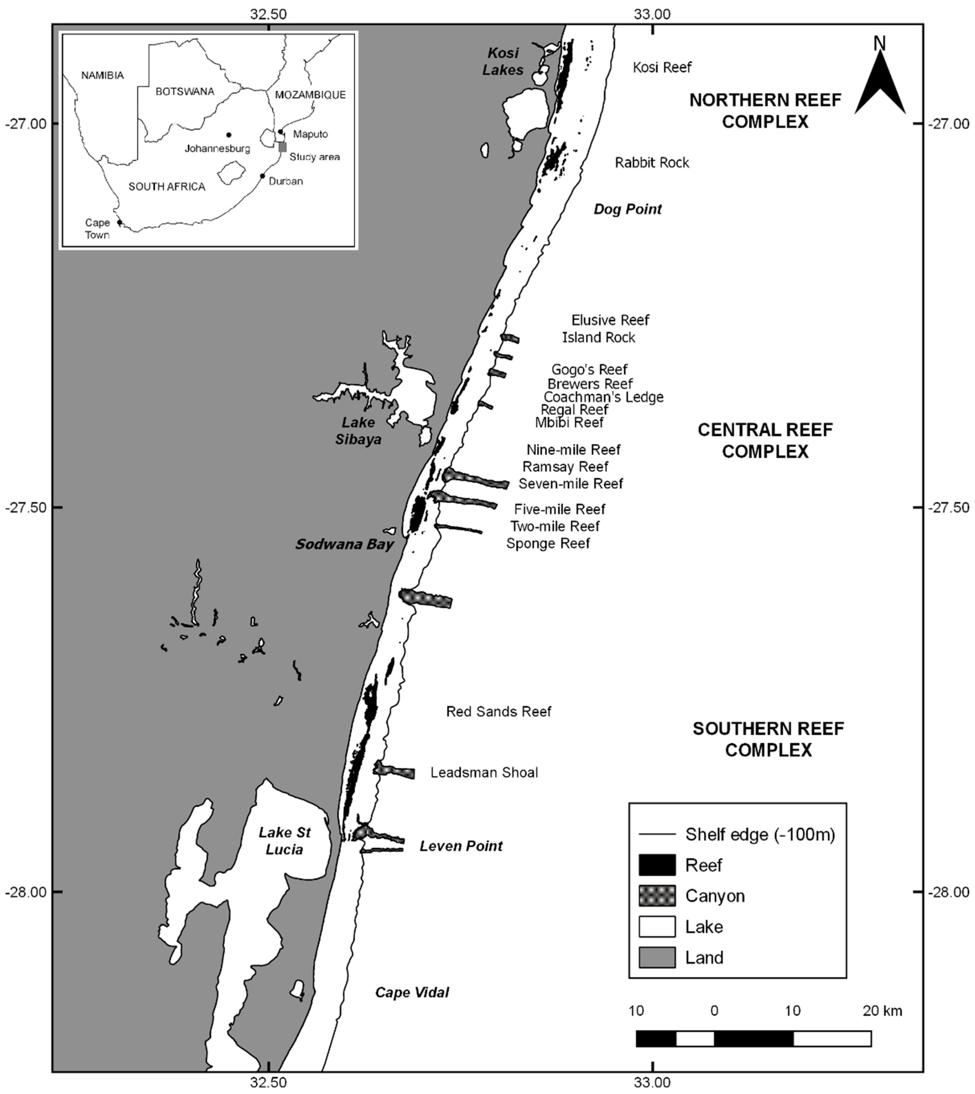
The Maputaland reefs are located in the southwestern Indian Ocean, in its Delagoa Bioregion (Porter et al. 2013 [33]). They are non-accretive reefs composed of aeolinite beachrock derived from a submerged dune system (Ramsay and Mason, 1990 [34]). The reefs lie parallel to the shore and are distributed in three main areas, commonly referred to as reef complexes (Schleyer, 2000 [3]; Schleyer et al. 2018 [4]) (Figure 1). The oceanographic characteristics of this bioregion and the reasons coral communities flourish in it have been investigated by Porter et al. (2017a [15]). The reefs are bathed by warm oceanic waters from the confluence of the Mozambique and Southeast Madagascar currents that result in average temperatures of 24.4 °C (Porter and Schleyer, 2017 [16]). The extremely narrow (<3 km) continental shelf facilitates the intrusion of oceanic water which, together with the lack of riverine input, results in oligotrophic waters low in turbidity, chlorophyll, and nutrients (Porter et al. 2017a [15]). The shelf edge is broken by a total of 11 submarine canyons of varying age and size (Ramsay, 1994 [28]). The shelf edge and canyons interact regularly with large southward moving eddies (Morris et al. 2013 [27]). The physical characteristics of the reefs themselves have been described in detail by Schleyer and Porter (2018 [14]).
On the shallower inshore western side of the reefs, frequent sand movement facilitated by large swells plays a key disturbance role that regulates communities (Porter et al. 2017a [15], b [20]; Schleyer et al. 2018 [4]). The westward land boundary is characterised by a sandy coastal plain with extensive lakes and wetlands, which are separated from the reefs by a narrow dune cordon (Grundling et al. 2013 [35]). These wetland lakes leach freshwater and dissolve nutrients and pollutants into the coastal zone (Meyer et al. 2001 [24]; Smithers et al. 2017 [25]; Porter et al. 2018a [26]). The reefs are therefore wedged between two contrasting and dynamic disturbance regimes across the narrow shelf—a dynamic coastal environment on their west side and a fluctuating oceanic environment on their east side.
2.2. Reef Community and Environmental Data
2.2.1. Reef Community Surveys
Surveys of the Maputaland reefs were undertaken over a six–year period from 1999 to 2005 at haphazardly chosen sites so that there was no bias or correlation between time and latitude or location. Only negligible bleaching of the coral communities was recorded during this time, and there was no bleaching-related mortality attributable to the warm regional temperatures of 1998, 2000, and 2005 (Schleyer and Celliers, 2000 [36]; Celliers and Schleyer, 2002 [37]; Sebastián et al. 2009 [38]). As there are no significant rivers in the region and the reefs are relatively deep (>12 m), there were no major siltation, rain inundation, storm events, or any discernible effects on communities in the region during the six-year sampling period.
The specifics of these surveys are detailed by Schleyer and Porter (2018 [14]), but sites within all three reef complexes were surveyed along the coast from −26.9° to −27.8° (Figure 1 and Electronic Supplementary Material 1). In brief, coral communities were surveyed along haphazardly-placed transects using a modified quadrat and rapid photographic technique with a digital camera whilst on SCUBA (English et al. 1994 [39]; Celliers and Schleyer, 2002 [37]). A spacer bar was attached to the camera, and high-resolution, vertically-orientated photo-quadrat images of 0.35 m2 were recorded of the reef at regular intervals along transects. Sample size and resolution were increased using a subsampling strategy that combined the data from at least 20 (average 23.5) consecutive photo-quadrat frames to provide an individual transect for analysis (Schleyer and Celliers, 2005 [9]). A total of 419 georeferenced transects were surveyed across 17 reefs in the region, thus providing 9860 photo-quadrats for analysis.
Data on the benthic composition of the reefs were extracted from each photo-quadrat image using a regular grid of points (Carleton and Done, 1995 [40]). Ten fixed and evenly distributed grid points were superimposed onto each photo-quadrat, and the benthos or substratum beneath each point was identified to species (if possible) or taxon. The number of intercepts in each taxonomic or substratum category was considered to be directly proportional to the planar area covered by that particular category within each quadrat, thereby allowing the calculation of percentage cover at the quadrat level. The community composition data utilised in these analyses are documented in fine scale by Schleyer and Porter (2018 [14]) and consisted primarily of soft and hard corals as well as turf algal communities.
2.2.2. Environmental Variables Associated with Reef Communities
Four environmental explanatory variables and a set of spatial explanatory variables (parameters) were considered in models. The environmental variables can be considered surrogates for several abiotic variables as they are not direct drivers of species distributions. Rather, they act as surrogates for other variables that are assumed to, or are known to, directly or indirectly influence reef organisms. For example, depth is not a direct driver but acts as a surrogate for light attenuation and wave action.
The four environmental variables included were depth, the proximity and size of submarine canyons, distance to the high-tide mark, and distance to the shelf edge. The depth of each transect was derived from a spatially interpolated model of a bathymetric grid surveyed using side-scan sonar (see Schleyer and Porter, 2018 [14]). Distances were calculated between the midpoint of each transect and the high-tide mark and the shelf edge using the v.distance geoalgorithm (GRASS-GIS 7). The high-tide mark shapefile layer was acquired from the Ezemvelo KZN Wildlife Coastal and Marine biodiversity plan (SeaPlan; EKZNW, 2009 [41]) and provides the maximum height attained during spring high tide in a region where the height between spring and neap tides rarely exceeds 2 m (SAN-HO, 2019 [42]). The shelf edge shapefile layer was the continental shelf break used in the 2011 South African National Spatial Biodiversity Assessment corresponding to the 100-m depth contour in the region (Harris et al. 2012 [43]; Sink et al. 2012 [44]). For the influence of canyons, we derived a repeatable and relative metric called the ‘canyon effect’ for each transect based on the distance a particular transect was located from each canyon in the region with consideration of the sizes of the canyons. The metric was calculated for each transect as follows, so that canyons that were large and relatively close to transects would have a greater effect than relatively small canyons further away:
where Si is the footprint size of each of the 11 canyons and Di is the distance between a particular transect and each of the 11 canyons. The locations and sizes of the various canyons in the region were obtained from the canyon layer used in the 2018 South African National Biodiversity Assessment. Canyons located more than 50 km either north or south of the northernmost and southernmost transects, respectively, were ignored. All geospatial analyses were conducted with Quantum GIS version 2.18 using the longitude-orientated projected coordinate system with the central meridian set to 33° and WGS84 as the reference ellipsoid.
2.3. Data Analysis
2.3.1. Reef Communities
The average percentage cover of each taxon or substratum type per transect was calculated based on replicate quadrats as a basis for further statistical analysis. This resulted in a biotic matrix (after removal of substratum type) of 419 rows (transects) by 107 columns (taxa). Relationships among reef communities in the transects were displayed using a non-metric multidimensional scaling ordination based on the Bray-Curtis similarity distance metric. The percentage cover ± standard deviation of each taxon, as well as several functional groups (algae, soft corals, hard corals, ascidians, sponges, and echinoderms) contributing to the total living cover on Maputaland reefs, was then calculated from the 419 transects.
2.3.2. Environmental and Spatial Variables Associated with Reef Communities
Summary statistics for the region and for each of the three reef complexes were calculated for the four environmental variables and two spatial variables, longitude and latitude, based on transects as replicates. Pearson product moment correlations and draftsman plots were also assessed between the environmental and spatial variables to check for multicollinearity and redundancy prior to incorporating them into explanatory models. A principal component analysis was undertaken on the normalised (zero mean and unit variance) environmental and spatial data (longitude and latitude) derived from each transect to visualise the multivariate characteristics associated with transects from the different reef complexes. A second principal component analysis was conducted on the same environmental data, except that a set of spatial parameters (see below) derived from the longitude and latitude coordinates were used instead. This latter analysis was undertaken to provide visualisation of the most important (in terms of their strength) spatial parameters associated with the first two dimensions of the ordination and their relationships with the environmental variables.
2.3.3. Spatial Parameters and Distinguishing them from Environmental Effects
Patterns in reef community composition may result from the dependence of taxa on environmental variables and/or from community-based processes such as competition or recruitment (Dray et al. 2006 [45]). In order to distinguish between these two types of processes because of spatially-structured environmental variation, it is necessary to explicitly incorporate spatial relationships into models. In regression-type models linking community metrics to a suite of explanatory variables, independence among sampling units may be violated due to spatial autocorrelation resulting in inflated type 1 errors. Spatial autocorrelation is defined by Legendre (1993 [17]) as the property of random variables taking values at pairs of locations a certain distance apart that are more similar (positive autocorrelation) or less similar (negative autocorrelation) than expected for randomly associated pairs of observations. In our transect data, reef communities in one transect may be influenced by the communities from neighbouring transects due to contagious biological processes. Similarly, environmental variables characterising transects are unlikely to be randomly or uniformly spatially distributed, but they are structured in a manner that results in gradients (e.g., depth) or patchy structures (e.g., locations of reefs).
As such, we mitigated the effects of spatial autocorrelation in our analyses by explicitly incorporating the spatial structure of our data into the modelling procedure. Rather than using a matrix of the third-degree polynomial functions of the geographic coordinates of the transects to account for spatial structure, such as in trend surface analysis (see Borcard et al. 1992 [46]), we employed a different approach appropriate for the irregular and patchy locations of our samples and the potentially complex spatial structure of the environmental variables that influence the reef communities (Scarlett, 1972 [47]; Legendre and Legendre, 1998 [18]).
In deriving spatial explanatory variables, we adopted a data-driven approach and used the principle coordinate analysis of neighbour matrices (PCNM) method to account for space in the analysis (Borcard and Legendre, 2002 [48]; Dray et al. 2006 [45]). The method involves calculating a spatial weighting matrix among transects before eigenvectors are extracted that maximise the Moran’s index of spatial autocorrelation (Dray et al. 2006 [45]). A Delaunay triangulation neighbourhood matrix derived from the projected geographic coordinates of each transect was used to truncate a Euclidian distance matrix of the projected transect coordinates before the principal coordinates were calculated (Legendre and Legendre, 1998 [18]; Dray et al. 2006 [45]). This Euclidian distance matrix was then weighted according to the distances between transects using the function:
where d is the distance between the ith and jth transects. This resulted in a spatial weighting matrix comprising 419 principle coordinate explanatory variables that represented the spatial structures among the 419 transects at all scales. Unlike the original PCNM method developed by Borcard and Legendre (2002 [48]), the principle coordinates associated with the negative eigenvalues are retained as spatial descriptors (see Dray et al. 2006 [45]). The multivariate spatial matrix was then further reduced in dimension using a data-driven procedure. This involved selecting an optimal set of eigen vectors for the spatial model based on the corrected Akaike information criterion by comparing the original spatial weights matrix of 419 variables with the species-by-transect matrix (Dray et al. 2006 [45]). The resulting parsimonious spatial weights matrix consisted of 75 spatial variables (parameters) for incorporation into further analyses.
2.3.4. Environmental and Spatial Effects on Reef Communities
The potential roles of environmental variables and spatial effects in structuring the reef communities were determined using a series of distance–based linear models that allowed us to partition the variability into environmental and spatial categories, as well as according to the four individual environmental variables. The approach used follows that described in Borcard et al. (1992 [46]), where the spatial component of the ecological variation in communities can be partialled out. In total, three matrices were utilised: Species assemblages at each of the 419 transects (107 × 419), environmental variables (4 × 419), and a spatial weights (75 × 419) matrix derived from the PCNM based on the geographical coordinates of the transects.
Four multivariate distance-based linear models (DISTLM) were constructed from a Bray-Curtis similarity distance matrix of the species assemblages, each constrained by a set of explanatory variables. The procedure implemented by DISTLM is a distance-based redundancy analysis (dbRDA) based on the method of Legendre and Anderson (1999 [49]), with further refinement by McArdle and Anderson (2001 [50]). By using a set of environmental explanatory variables and a set of spatial variables, the effects of the environmental variables and the spatial structure that is dependent on them (because of spatially-structured environmental variation) can be isolated by making two canonical ordinations. Consequently, we were able to partition the variation in reef communities according to (Legendre, 1993 [17]): (1) Non-spatial environmental variation, (2) spatially-structured environmental variation, (3) spatial variation that does not correspond to the environmental variables, and (4) unexplained, non-spatial variation.
Model 1 involved constraining the species matrix using the four environmental variables as predictor variables and employed a step-wise regression selection procedure with 9999 permutations and the adjusted-R2 value as the selection criteria. Model 2 involved constraining the species matrix by the spatial weights matrix of 75 variables employing the same selection procedure and permutations used in Model 1. Model 3 was similar to Model 1 after removing the effects of space and was thus a partial dbRDA. In Model 3, we fitted the 75 spatial parameters first as a complete group (known as indicator variables in PERMANOVA+ for PRIMER) before the environmental variables were fitted with a step-wise selection procedure. Finally, Model 4 was similar to Model 2 after removing the effects of the four environmental variables. In Model 4, we performed a second partial dbRDA by incorporating the four environmental variables into a group which we fitted first before the 75 spatial parameters were fitted with step-wise selection. Consequently, Models 3 and 4 are partially redundant and can be used to factor in spatial autocorrelation and to partition the variation into environmental and spatial components (Borcard et al. 1992 [46]).
Marginal tests were included as well as sequential tests in all four models. The amount of variation accounted for by the sequential tests was used to partition variation into spatial and environmental components successively as follows (see Borcard et al. 1992 [46]):
Equation (1) = Non-spatial environmental variation:
Equation (2) = Spatially structured environmental variation:
Equation (3) = Spatial species variation not shared by environmental variables:
Equation (4) = Unexplained variation:
where Vi is the amount of variation explained by each of the environmental and or spatial parameters in sequential tests.
The overall proportion of explained variation in reef community composition was calculated by summing the cumulative variation derived from the sequential tests of Models 1 and 4 (Borcard et al. 1992 [46]). The models were viewed using distance-based redundancy analysis (dbRDA) plots. Statistical analyses were conducted in R 3.0.3 (R Core Team, 2018 [51]), using the packages spdep and tripack, and in PERMANOVA+ for PRIMER, version 7 (Dray et al. 2006 [45]; Renka and Gebhardt, 2013 [52]; Anderson et al. 2008 [53]).
3. Results
3.1. Community Structure and Composition
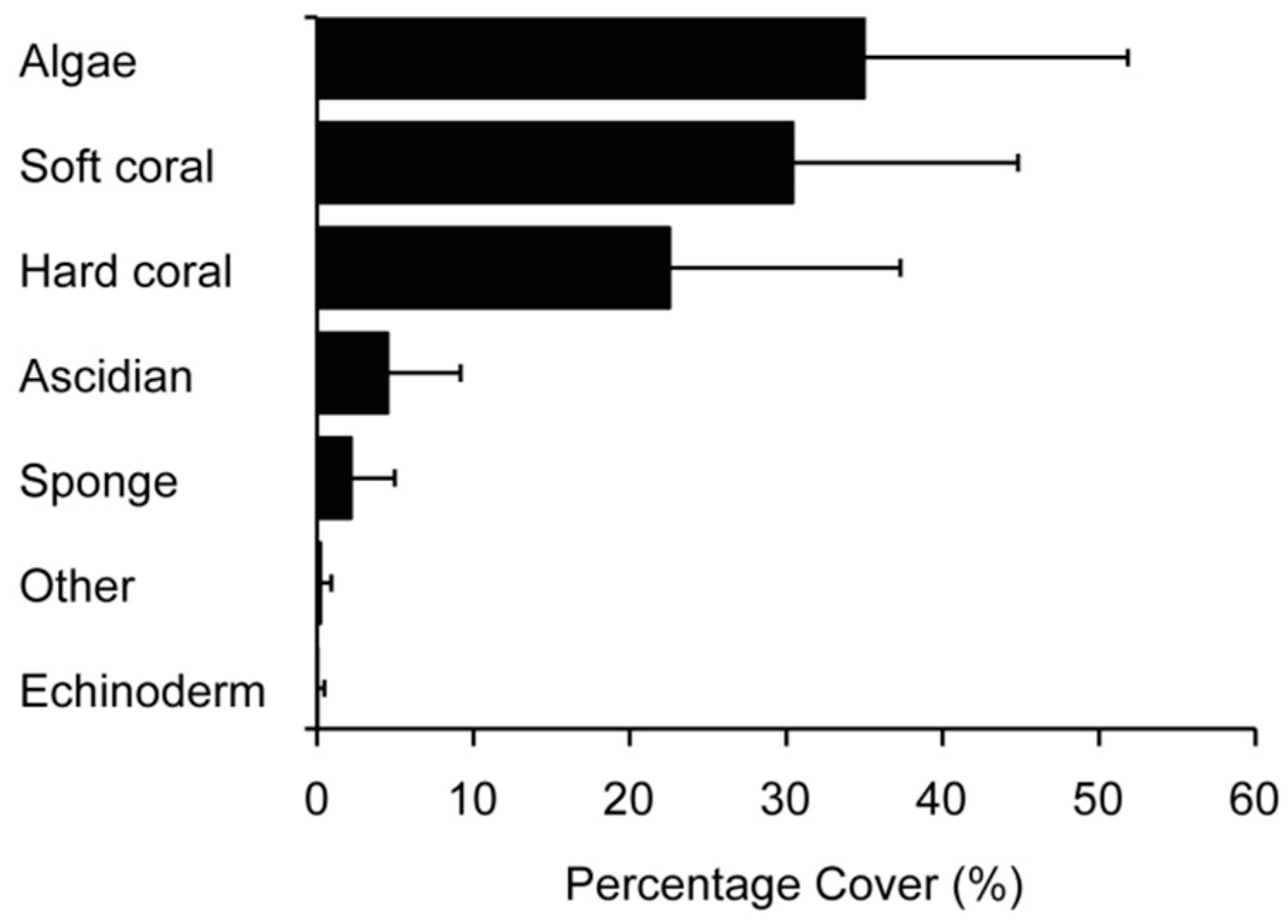
Corals dominated the Maputaland reefs, with an average ± standard deviation (SD) soft coral percentage cover of 30.4 ± 14.4% and hard coral cover of 22.5 ± 14.7% (Figure 2). Algae, largely in the form of turf communities, also made a notable contribution, comprising 35.0 ± 16.8% of the living cover. Groups that made minor contributions were the ascidians (4.5 ± 4.7%) and the sponges (2.2 ± 2.8%).
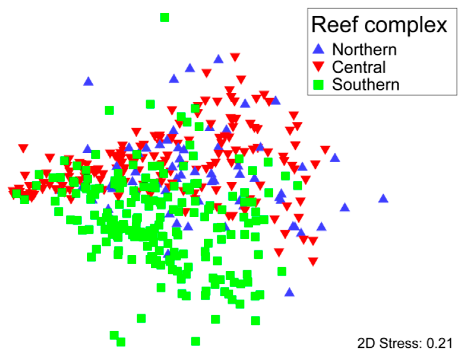
Non-metric multidimentional scaling ordination of the percentage cover of different taxa surveyed in transects did not show distinct groupings into separate reef complexes (Figure 3). There was considerable overlap between communities from the Northern and Central Reef Complexes. The Southern Reef Complex was the most distinct with relatively less overlap compared to the Northern and Central Reef Complexes.
Several species of Sinularia, especially S. abrupta (3.4 ± 3.9%), in addition to Sarcophyton spp. (3.6 ± 3.9%) and Lobophytum spp. (1.3 ± 2.0%) contributed most to the overall percentage cover of soft corals (Figure 4). Montipora spp. (5.5 ± 5.4%), Echinopora gemmacea (1.7 ± 3.9%), Acropora austera (1.5 ± 4.0%), and Favites spp. (1.5 ± 1.3%) were the main taxa contributing to the cover of hard corals. The solitary ascidian Polycarpa mytiligera (2.5 ± 3.5%) also made a notable contribution to the total living cover.
3.2. Environmental and Spatial Characteristics of Reef Transects
The average ± standard deviation of the canyon effect was highest for the Central Reef Complex (5616 ± 2181) and lowest for the Northern Reef Complex (812 ± 88) (Table 1). The maximum canyon effect values showed a similar pattern, being lowest in the Northern Reef Complex (907) and highest in the Central Reef Complex (9842). The average depths of the reef complexes were similar, as were the average distances they were located from the high-tide mark on land (no reefs break the surface). The average distance to the shelf edge was similar between the Central (2445 ± 411 m) and Southern (2624 ± 466 m) Reef Complexes but considerably further away for the Northern Reef Complex (4563 ± 759 m). The reef complexes extended from 2977 to 3086 km southwards from the equator and were found to lie in a north-north-east direction 11 to 33 km west of 33°.
Exploratory correlation analyses between all pairs of environmental variables revealed limited autocorrelation between them. Pearson correlation coefficients were ≤0.75 indicating negligible redundancy and suitability for incorporation into multivariate models (ESM 3) (Anderson et al. 2008 [53]). Longitude and latitude were, however, strongly correlated (r = 0.99).
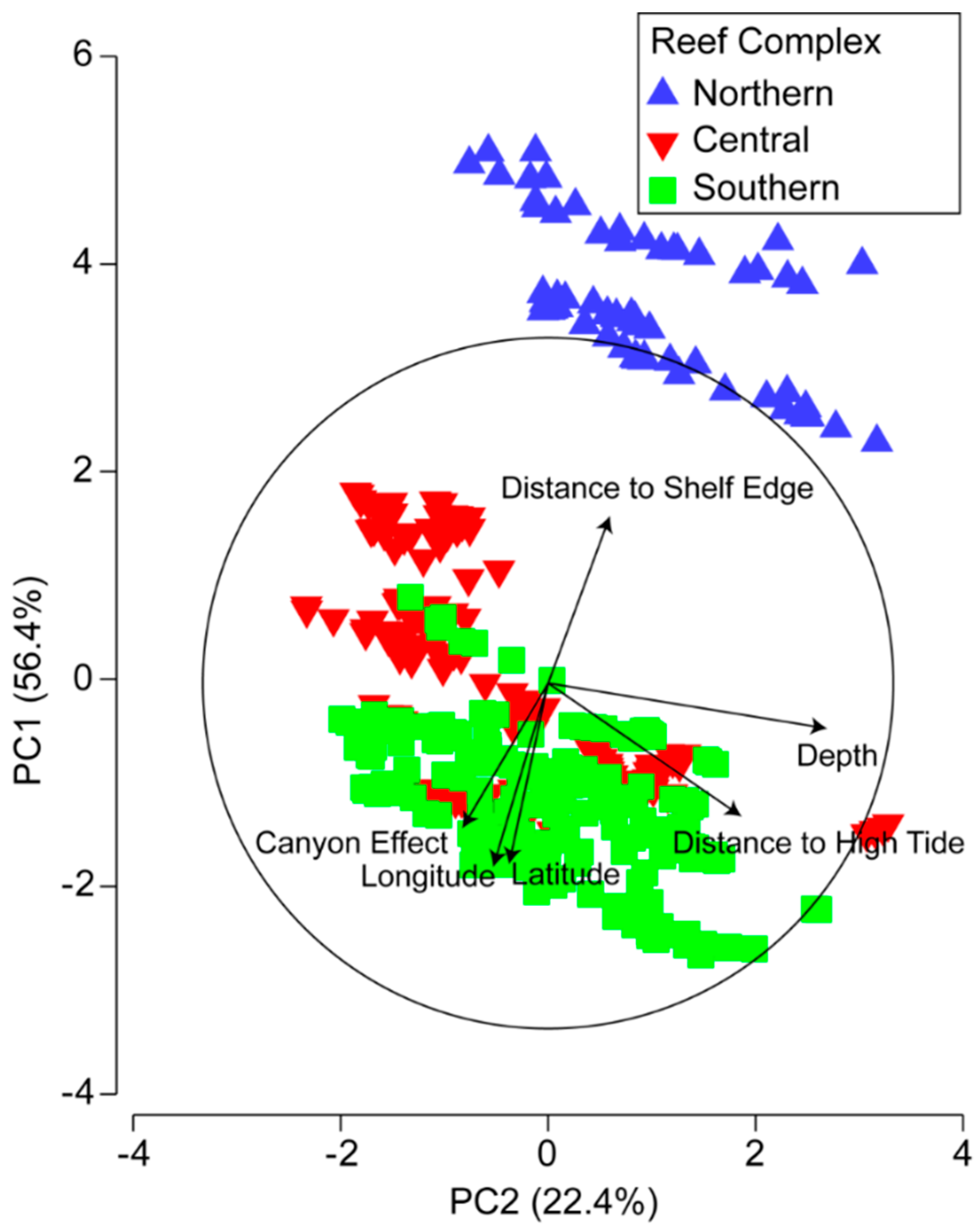
Principle components analysis based on the environmental variables and the two spatial variables longitude and latitude indicated a clear distinction between transects from the Northern Reef Complex and transects from the Central and Southern Reef Complexes, which formed a separate group. There was clear separation between these two groupings on principal component (PC) 1 (y-axis) according to their locations (both latitude and longitude) and distances from shelf edge and the canyon effect (Figure 5 and Table 2). Within each of the three complexes, transects separated out on PC 2 (x-axis) largely due to their depth and, to a lesser degree, their distance from the high tide mark. Together, principal components 1 and 2 accounted for the majority of variation (78.8%).
When the same analysis was conducted with the 75 spatial parameters derived from the latitude and longitude variables, far less variation could be accounted for in the first two dimensions of the principal components analysis (ESM 4, Figure S1). The Northern Reef Complex again separated out from the Central and Southern Reef Complexes, but the inclusion of a set of spatial parameters resulted in further dispersion of the transects in general in all three complexes. Spatial parameter S1 demonstrated the strongest eigenvector with PC 1 (0.264) and was highly positively correlated with both longitude (r = 0.54) and latitude (r = 0.52), as was S5 (ESM 4, Figure S2). Spatial parameter S6 had the strongest eigenvector on PC 2 (0.416) and exhibited modest negative correlations with both longitude (r = −0.19) and latitude (−0.17).
3.3. Environmental and Spatial Effects on Reef Communities
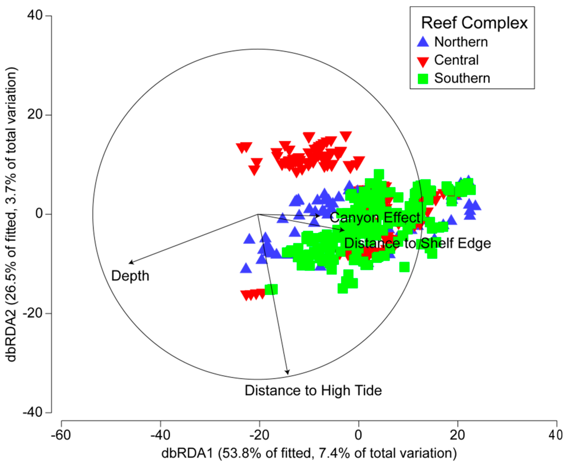
Marginal tests of the individual environmental variables (Model 1) indicated that all four accounted for significant amounts of variation in reef communities (P < 0.0005) (Table 3). Depth and distance to high tide accounted for most of the variation, followed by distance to shelf edge and the canyon effect. Sequential tests indicated that a total of 13.8% of the community structure could be explained by the environmental variables, with all four variables contributing significant effects (P < 0.0005) (Table 3). The distance-based redundancy analysis (dbRDA) ordination of the first two axes accounted for 80% of the fitted variation (11% of the total variation) (Figure 6). There was strong separation in community structure along a depth gradient as well as distance to shelf edge on axis 1; the similar seperation occurred with distance to high tide on axis 2.
Marginal tests of the 75 spatial parameters (Model 2) indicated significant correlation for many of them with reef community structure (P < 0.01), with the top five each accounting for 2.5–4.5% of community variation (ESM 5, Table S1). Sequential tests of the spatial parameters revealed that S5, S2, and S1 accounted for most (11.5%) of the cumulative variation in reef community composition and were significantly correlated with it (P < 0.0005) (ESM 5, Table S2). The total explained cumulative variation was 50.2%. The dbRDA ordination of the first two axes accounted for 59% of the fitted variation (30% of the total variation) (ESM 6, Figure S1). There was strong separation in community structure according to S5, as well as S1 on axis 1 and S 2on axis 2.
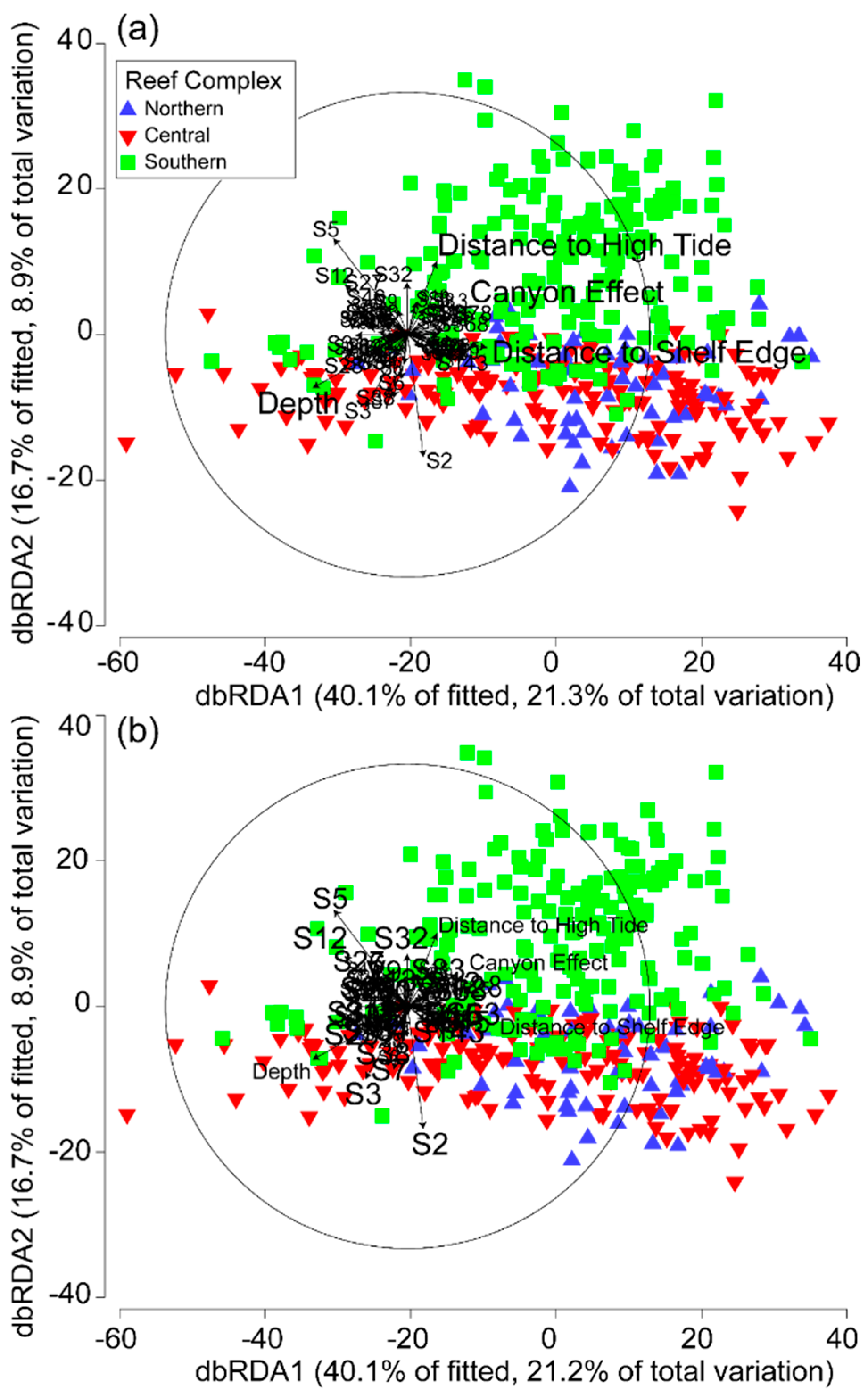
Marginal tests of the first partial model (Model 3) confirmed the results of Models 1 and 2 (ESM 7, Table S1). Sequential tests investigating non-spatially structured environmental variation indicated that all four environmental variables were significantly correlated with community composition after the effects of space were removed (P < 0.0005) (Table 4). In this regard, depth followed by distance to high tide accounted for most of the non-spatially structured environmental variation correlated with reef communities out of the four environmental variables investigated. In total, the non-spatial component of the four environmental variables explained 3% of the total variation in reef communities. The dbRDA ordination of the first two axes accounted for 57% of the fitted variation (30% of the total variation) (Figure 7a). There was strong separation in community structure according to depth as well as distance to shelf edge and, to a lesser degree, the canyon effect on axis 1; the similar seperation occurred with distance to high tide and depth on axis 2.
Marginal tests of the second partial model (Model 4), confirmed the results of Models 1 and 2 (ESM 8, Table S1). Sequential tests investigating spatial variation not shared by environmental variation indicated that half of the spatial parameters were significantly correlated with community composition after the effects of the four environmental variables were removed (P < 0.01), with the majority of others being borderline (ESM 8, Table S2). In this regard, S5 followed by S2 accounted for most of the spatial variation not shared by any of the environmental variables associated with reef community structure and correlated significantly with it (P < 0.0005). In total, the spatial variation not shared by any of the environmental variables explained 39% of the total variation in reef communities. The dbRDA ordination of the first two axes accounted for 57% of the fitted variation (30% of the total variation) and was almost identical in appearance to the dbRDA ordination derived from Model 3 (Figure 7b). There was strong separation in community structure according to S5 as well as S12 on axis 1, and S5 and S2 on axis 2.
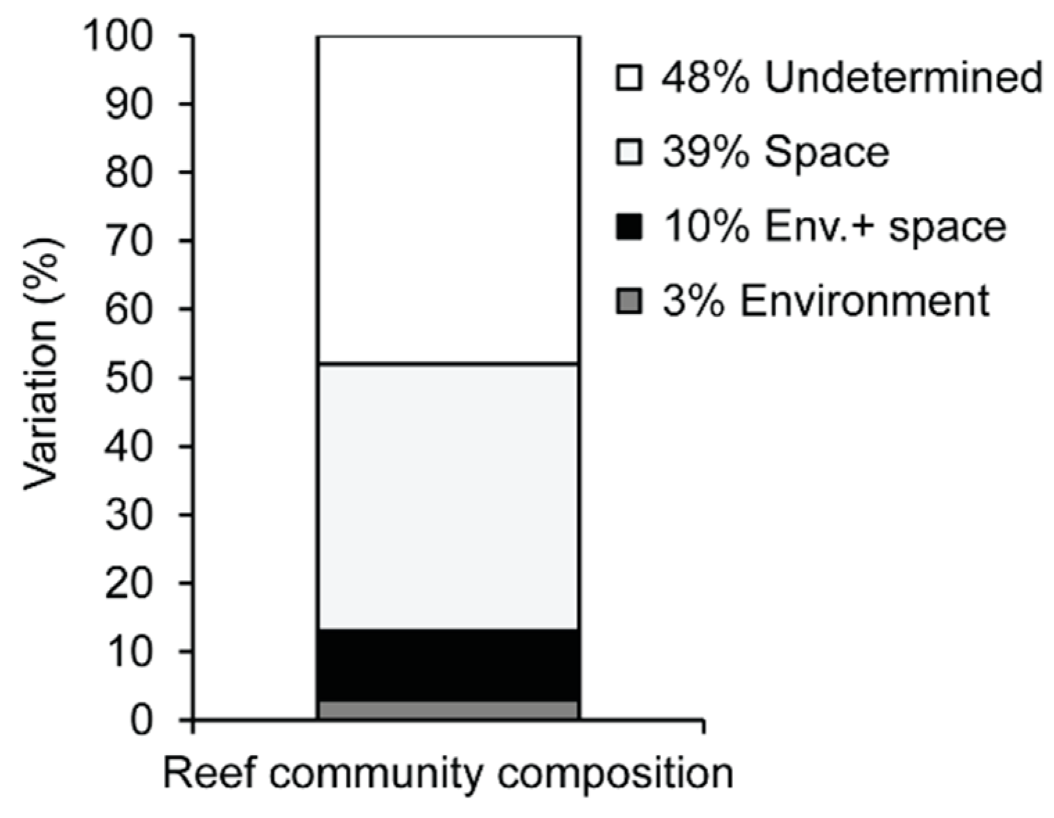
When the results of the four models were combined, 52% of the total variation in community structure could be accounted for (Figure 8). Space accounted for the majority (39%) of the explained variation in reef community structure followed by spatially structured environmental variation (10%) attributable to the four environmental variables investigated. Pure environmental variation (not spatially structured) explained 3% of the total variation in reef communities.
4. Discussion
4.1. Summary of Findings
Both soft and hard coral dominated reef communities, comprising 52% of the community composition. The four environmental variables combined accounted for 13% of the variation in coral community composition. Of this variation, 10% was spatially structured. Depth accounted for marginally more variation compared to the other three environmental variables. All of these variables nevertheless correlated significantly with the composition of the coral communities, even when the effects of spatial autocorrelation were accounted for. A large proportion (39%) of the variation in coral communities was accounted for by their spatial location indicating that other ecological processes (environmental and biological) which are spatially structured are playing a role. A total of 48% of the variation in the coral communities could not be accounted for by the environmental and spatial variables incorporated in the models.
4.2. Environmental and Spatial Effects
The spatial turnover of reef communities was determined using partial distance-based linear modelling using a set of 75 spatial parameters derived from geographical coordinates that described the spatial pattern exhibited by coral assemblages in the most parsimonious way. The spatial variation that was not related to any of the four environmental variables investigated accounted for approximately 39% of the reef community variation (i.e., 75% of explained variation). This relatively high amount of ‘unrelated’ spatial variation indicates elevated levels of associated biological processes lacking any form of relationship with the four environmental variables included in the analysis. The unrelated spatial variation could be attributable to spatial patterns in biotic processes such as recruitment, growth (Burn et al. 2018 [54]), survivorship, predation (Hamman, 2018 [55]), aggregation of intraspecific planulae and adults (Williams, 1976 [56]; Goreau et al. 1981 [57]; Karlson et al. 2007 [58]), competition for space (Chadwick and Morrow, 2011 [59]), self-seeding (Miller and Ayre, 2008 [60]; Gilmour et al. 2009 [61]), or abiotic variables not investigated that are spatially structured to varying degrees (Kieth et al. 2013 [62]; Porter et al. 2017a [15]; Schleyer and Porter, 2018 [14]).
Significant biological disturbances on these reefs appear to be rare. However, crown-of-thorns starfish (COTS) (Acanthaster planci) outbreaks occurred between 1994–1999 and had acute but very localised effects (Schleyer, 1998 [63]). Alveopora spp., Montipora spp. and various Favidae were preyed on the most, although some soft corals and sponges were also consumed (Celliers and Schleyer, 2006 [64]). Several coral diseases occur on the reefs, and, although their prevalence is low (~4% of coral colonies are affected), they may nevertheless exert significant biological pressure (Séré et al. 2012 [65]; Séré et al. 2015 [66]). Porites spp., Hydnophora spp., and Pocillopora spp. appear to be the most susceptible genera.
Coral recruitment on these high latitude reefs is known to vary both spatially and temporally (Glassom et al. 2006 [67]). Recruitment rates vary widely both within and between different reefs, with some reefs exhibiting persistently low levels of recruitment. Patterns of variation are also inconsistent between seasons. Recent genetic analyses of the scleractinians Platygyra daedalea and Acropora austera have found that there is likely to be an important degree of self-seeding in South African populations. High-latitude coral communities are frequently known to be genetically isolated, and the South African coral reefs appear to follow this pattern (Macdonald et al. 2010 [68]; Montoya-Maya et al. 2016 [21]). High levels of relatedness have also been found between closely-spaced colonies of A. austera, suggesting that larval dispersal may be limited to tens of metres. The non-random spatial recruitment dynamics that have been shown by Glassom et al. (2006 [67]) and Hart (2011 [69]) on these reefs, coupled with the genetic patterns discovered by Montoya-Maya (2014 [22]), indicate that the coral larvae of P. daedalae and A. austere—and probably other species—settle close to natal or kin colonies. This is likely to be manifested in clustered distributions of colonies that are in turn gradually distributed over the reefs non-randomly, thereby displaying different scales of spatial autocorrelation within reefs as well as across the latitudinal gradient of the three reef complexes.
In addition, the reef organisms and corals themselves may be regulating the spatial structure of the reef communities due to competitive interactions (Sammarco et al. 1985 [70]; La Barre et al. 1986 [71]; McCook et al. 2001 [72]). As these reef communities are dominated by soft corals, which are known to have allelopathic chemicals that facilitate interspecific competitive interactions, they may play a particularly prevalent role in governing what other species of coral grow adjacent to them (Sammarco et al. 1983 [73]; Changyun et al. 2008 [74]). This can provide soft corals a competitive advantage over hard corals (Sammarco et al. 1983 [73]). Besides allelopathic chemicals, coral larvae are also known to have an affinity to settle on crustose coralline algae, which is also likely to result in a measure of relatively fine-scale spatial structure in coral communities (Fabricius and De’ath, 2001 [75]).
Of the environmental variation that could be explained and related to reef communities, 77% was spatially structured. The shallow reef communities therefore have a measure of spatial dependence on the explanatory abiotic variables we investigated. This is not surprising, since the four environmental variables are stationary and do not change their locations in time—the location of the high-tide mark is temporally fixed, as are the distances between reef communities and the shelf edge and canyons. However, the remaining 23% of the explained environmental variation that was not spatially structured (i.e., pure environmental variation) is most likely due to the variable effect that the four variables may exert over time in structuring reef communities. For example, the magnitude of the canyon effect may vary not only in the distance that a reef community is from a canyon, but in time too, as cold water is only likely to be periodically upwelled and funnelled via canyons onto the shallow reefs during Ekman, veering when the meandering current flows close to the shelf edge (Hsueh and O’Brien, 1971 [76]; Roberts et al. 2006 [77]).
Across the shelf, depth accounted for most of the variation in reef community composition, followed by distance to the high-tide mark and shelf edge. The canyon effect played a subordinate role, yet was nevertheless significantly correlated to community composition even when spatial autocorrelation was accounted for, as was the case for all the other explanatory variables investigated. Depth is well known to be a key factor that indirectly influences communities on these marginal reefs in particular, as they are light-limited in winter due to their high-latitude and experience large swells, the effects of both of which diminish with depth (Porter et al. 2017a [15]; Schleyer et al. 2018 [4]).
The distance to the high-tide mark is probably a surrogate for gradients of retention and remobilization of sediments, with accompanying increases in disturbance and reduced coral larval settlement. It would also be associated with other factors such as wave reflection, refraction, and energy retention, as well as oceanic influences; it was only weakly correlated with depth (Graus and Macintyre, 1989 [78]; Birrell et al. 2005 [79]; Kench and Brander, 2006 [80]; Porter et al. 2017a [15], b [20]). Distance offshore was similarly a key factor in explaining the diversity of coral reef organisms across the relatively wide continental shelf of the Spermonde Archipelago, Indonesia (Cleary et al. 2005 [81]).
Based on the abiotic characteristics of the three reef complexes, the Northern Complex is probably the most thermally stable as its reefs are furthest from any canyons (i.e., the lowest canyon effect), and are also furthest away from the shelf edge which interacts with warm south-moving eddies and deeper cooler waters (Morris et al. 2013 [27]). This may explain why relatively temperature-sensitive species such as branched acroporids (e.g., A. austera and Acropora hyacinthus) are more abundant in the Northern Complex compared to the Central and Southern Complexes (McClanahan et al. 2007 [82]; Schleyer and Porter, 2018 [14]). Long-term temperature monitoring in the Central Reef Complex has indeed revealed that it is characterised by rapid temperature fluctuations on an hourly basis (Porter and Schleyer, 2017 [16]). It was, however, impractical to include in-situ or remotely-sensed temperatures in our models due to the large number of transects and their relatively close proximity to each other.
Though the Northern Complex may be the most thermally stable of the three complexes, it is likely to be the warmest, as indicated by the decreasing trend in bleaching index with increased latitude that has been recorded in the region (Porter et al. 2018b [83]). Nevertheless, bleaching has up to now played only a minor role on these high-latitude reefs, as levels have never been recorded to exceed ~10% of the coral or living cover but may promote disease and infection, thereby affecting competitive interactions (Celliers and Schleyer, 2002 [37]; Séré et al. 2015 [66]; Porter et al. 2018b [83]).
4.3. Unexplained Variation
The amount of unexplained variation in reef communities is relatively high, but not uncharacteristic of ecological studies, because species abundance data are typically very noisy (Guisan and Zimmermann, 2000 [84]). These underlying and unexplained processes are at least partly uncorrelated with the set of measured environmental explanatory variables we included and were not totally predictable by any form of spatially structured environmental drivers as far as the 75 spatial parameters we incorporated as synthetic descriptors could explain. It is probable that a large amount of the unexplained variation in community composition is due to a combination of unquantified abiotic and/or biotic variables that have either contemporary or had an historical influence, resulting in spatial structures that have not been captured by the parsimonious model of spatial parameters. For example, several contemporary abiotic characteristics associated with the local reef physiognomy (e.g., slope, aspect, reef susceptibility to sand inundation) are correlated with coral communities to varying degrees and may not fully exhibit spatial structure captured by the spatial parameters (Porter et al. 2017a [15]; Schleyer and Porter, 2018 [14]). Furthermore, the spatial parameters were derived from the geographic coordinates of the mid-point along each transect line and may therefore not reflect the spatial scale at which finer-scale processes act.
In addition, a certain amount of unexplained variation may be due to stochastic processes in space and time. An example of this could be the stochastic nature of storm events that result in large amounts of sand abrasion, causing disturbance to communities (Porter et al. 2017a [15], b [20]). It is impossible to calculate the amount of unexplained variation that may have been explained by the addition of other environmental variables and spatial parameters, as these are probably due to spatiotemporal stochasticity that cannot be accounted for in deterministic models.
5. Conclusions
The four environmental variables explained a relatively small amount of the variation (13%) in the coral communities, as most of the variation was attributable to the spatial structure of the coral communities (39%) probably due to other spatially-structured, abiotic processes that were not measured and biotic processes that were not investigated. Nevertheless, both inshore and offshore factors (distance to high tide, distance to shelf edge, and the canyon effect) as well as depth were found to correlate significantly with coral reef community composition. These variables also displayed significant spatial autocorrelation in their associations with reef communities.
The South African coral communities therefore lie between a coastal disturbance regime on their western, inshore side and an oceanic disturbance regime on their eastern side along the shelf edge. The resulting level of disturbance by these processes is unlikely to be spatially and temporally consistent along the Maputaland coast due, in part, to the variable positions of the reefs, and it may demonstrate a north-south gradient of disturbance, which may in turn be manifested as a pronounced latitudinal gradient in coral community structure, as detected by Schleyer and Porter (2018 [14]). Conceptually, reefs in the Northern Complex appear to be exposed to relatively stable oceanographic conditions compared to reefs further south, but reefs in the Central and Southern Complexes are less likely to experience anomalously warm conditions due to an increased canyon effect and their proximity to the deeper and cooler waters of the shelf edge. This, conversely, would increase volatility in their temperature regime. The net relative effect is that the Northern Complex tends to be warm and stable, whilst the Central and Southern Complexes tend to be cool and unstable.
Supplementary Materials
The following are available online at https://www.mdpi.com/1424-2818/11/4/57/s1.
Author Contributions
Conceptualization and implementation, S.N.P.; data collection, M.H.S; formal analysis, S.N.P.; interpretation of results, S.N.P and M.H.S.; resources, M.H.S.; writing-original draft preparation, S.N.P.; writing-review and editing, M.H.S.
Funding
S.N.P. benefited from financial support in the form of employment from the South African Association for Marine Biological Research.
Acknowledgments
Three anonymous reviewers are thanked for their help with enhancing the manuscript. The authors acknowledge previous staff that assisted with field surveys, data extraction, and database management, in particular Louis Celliers and Angus Macdonald. Our gratitude to Kerry Sink of the South African National Biodiversity Institute and Tamsyn Livingston of Ezemvelo KZN Wildlife for provision of the relevant shapefile layers. We thank the South African Association for Marine Biological Research for their support.
Conflicts of Interest
The authors declare no conflict of interest.
References
- Laing, S.C.S.; Turpie, J.K.; Schleyer, M.H. Using SCUBA diving and boat-based angling to estimate an economic value of the coral reefs of Sodwana Bay, South Africa. Afr. J. Mar. Sci. 2019. under review. [Google Scholar]
- Laing, S.C.S.; Turpie, J.K.; Schleyer, M.H. Ecosystem services and coral reefs: An estimate of the value of sand generation and entrapment at Sodwana Bay, South Africa. Afr. J. Mar. Sci. 2019. under review. [Google Scholar]
- Schleyer, M.H. South African Coral Communities. Coral Reefs of the Indian Ocean: Their Ecology and Conservation; McClanahan, T., Sheppard, C., Eds.; Oxford University Press: Oxford, UK, 2000; pp. 83–105. [Google Scholar]
- Schleyer, M.H.; Floros, C.; Laing, S.C.; Macdonald, A.H.; Montoya-Maya, P.H.; Morris, T.; Porter, S.N.; Seré, M.G. What can South African reefs tell us about the future of high-latitude coral systems? Mar. Pollut. Bull. 2018, 136, 491–507. [Google Scholar] [CrossRef]
- Celliers, L.; Schleyer, M.H. Coral community structure and risk assessment of high-latitude reefs at Sodwana Bay, South Africa. Biodivers. Conserv. 2008, 17, 3097–3117. [Google Scholar] [CrossRef]
- Monniot, C.; Monniot, F.; Griffiths, C.; Schleyer, M. A monograph of the South African ascidians. Ann. S. Afr. Mus. 2001, 108, 1–141. [Google Scholar]
- Anderson, R.J.; McKune, C.; Bolton, J.J.; DeClerck, O.; Tronchin, E. Patterns in subtidal seaweed communities on coral-dominated reefs at Sodwana Bay on the KwaZulu-Natal coast, South Africa. Afr. J. Mar. Sci. 2005, 27, 529–537. [Google Scholar] [CrossRef]
- Schleyer, M.H.; Celliers, L. Biodiversity on the marginal coral reefs of South Africa: What does the future hold? Zool. Verh. 2003, 345, 387–400. [Google Scholar]
- Schleyer, M.; Celliers, L. Modelling reef zonation in the Greater St. Lucia Wetland Park, South Africa. Estuar. Coast. Shelf Sci. 2005, 63, 373–384. [Google Scholar] [CrossRef]
- Samaai, T.; Gibbons, M.J.; Kerwath, S.; Yemane, D.; Sink, K. Sponge richness along a bathymetric gradient within the iSimangaliso Wetland Park, South Africa. Mar. Biodivers. 2010, 40, 205–217. [Google Scholar] [CrossRef]
- Milne, R.; Griffiths, C. Invertebrate biodiversity associated with algal turfs on a coral-dominated reef. Mar. Biodivers. 2014, 44, 181–188. [Google Scholar] [CrossRef]
- Chater, S.A.; Beckley, L.E.; Garratt, P.A.; Ballard, J.A.; Van der Elst, R.P. Fishes from offshore reefs in the St. Lucia and Maputaland marine reserves, South Africa. Lammergeyer 1993, 42, 1–17. [Google Scholar]
- Floros, C.; Schleyer, M.H.; Maggs, J.Q.; Celliers, L. Baseline assessment of high-latitude coral reef fish communities in southern Africa. Afr. J. Mar. Sci. 2012, 34, 55–69. [Google Scholar] [CrossRef]
- Schleyer, M.H.; Porter, S.N. Drivers of soft and stony coral community distribution on the high-latitude coral reefs of South Africa. Adv. Mar. Biol. 2018, 80, 1–55. [Google Scholar] [PubMed]
- Porter, S.N.; Branch, G.M.; Sink, K.J. Changes in shallow-reef community composition along environmental gradients on the East African coast. Mar. Biol. 2017, 164, 101. [Google Scholar] [CrossRef]
- Porter, S.N.; Schleyer, M.H. Long-term dynamics of a high-latitude coral reef community at Sodwana Bay, South Africa. Coral Reefs 2017, 36, 369–382. [Google Scholar] [CrossRef]
- Legendre, P. Spatial autocorrelation—Trouble or new paradigm? Ecology 1993, 74, 1659–1673. [Google Scholar] [CrossRef]
- Legendre, P.; Legendre, L. Numerical Ecology, 2nd ed.; Elsevier Science: Amsterdam, NL, USA, 1998. [Google Scholar]
- Schleyer, M.H.; Celliers, L. Coral dominance at the reef–sediment interface in marginal coral communities at Sodwana Bay, South Africa. Mar. Freshwater Res. 2003, 54, 967–972. [Google Scholar] [CrossRef]
- Porter, S.N.; Branch, G.M.; Sink, K.J. Sand-mediated divergence between shallow reef communities on horizontal and vertical substrata in the western Indian Ocean. Afr. J. Mar. Sci. 2017, 39, 121–127. [Google Scholar] [CrossRef]
- Montoya-Maya, P.H.; Schleyer, M.H.; Macdonald, A.H. Limited ecologically relevant genetic connectivity in the south-east African coral populations calls for reef-level management. Mar. Biol. 2016, 163, 171. [Google Scholar] [CrossRef]
- Montoya-Maya, P.H. Ecological Genetic Connectivity between and within Southeast African Marginal Coral Reefs. Ph.D. Thesis, University of KwaZulu-Natal, Durban, South Africa, 2014. [Google Scholar]
- Mitchell, J.; Jury, M.R.; Mulder, G.J. A study of Maputaland beach dynamics. S. Afr. Geogr. J. 2005, 87, 43–51. [Google Scholar] [CrossRef]
- Meyer, R.; Talma, A.S.; Duvenhage, A.W.A.; Eglington, B.M.; Taljaard, J.; Botha, J.F.; Verwey, J.; Van der Voort, I. Geohydrological Investigation and Evaluation of the Zululand Coastal Aquifer; Water Research Commission Report 221/1/01; Water Research Commision: Pretoria, South Africa, 2001. [Google Scholar]
- Smithers, J.C.; Gray, R.P.; Johnson, S.; Still, D. Modelling and water yield assessment of Lake Sibhayi. Water SA 2017, 43, 480–491. [Google Scholar] [CrossRef]
- Porter, S.N.; Humphries, M.S.; Buah-Kwofie, A.; Schleyer, M.H. Accumulation of organochlorine pesticides in reef organisms from marginal coral reefs in South Africa and links with coastal groundwater. Mar. Pollut. Bull. 2018, 137, 295–305. [Google Scholar] [CrossRef]
- Morris, T.; Lamont, T.; Roberts, M.J. Effects of deep-sea eddies on the northern KwaZulu-Natal shelf, South Africa. Afr. J. Mar. Sci. 2013, 35, 343–350. [Google Scholar] [CrossRef]
- Ramsay, P.J. Marine geology of the Sodwana Bay shelf, southeast Africa. Mar. Geol. 1994, 120, 225–247. [Google Scholar] [CrossRef]
- Riegl, B.; Piller, W.E. Possible refugia for reefs in times of environmental stress. Int. J. Earth Sci. 2003, 92, 520–531. [Google Scholar] [CrossRef]
- Green, A. Sediment dynamics on the narrow, canyon-incised and current-swept shelf of the northern KwaZulu-Natal continental shelf, South Africa. Geo-Mar. Lett. 2009, 29, 201–219. [Google Scholar] [CrossRef]
- Morris, T. Physical Oceanography of Sodwana Bay and Its Effect on Larval Transport and Coral Bleaching. Master’s Thesis, Cape Peninsula University of Technology, Cape Town, South Africa, 2009. [Google Scholar]
- Riegl, B. Climate change and coral reefs: Different effects in two high-latitude areas (Arabian Gulf, South Africa). Coral Reefs 2003, 22, 433–446. [Google Scholar] [CrossRef]
- Porter, S.N.; Branch, G.M.; Sink, K.J. Biogeographic patterns on shallow subtidal reefs in the western Indian Ocean. Mar. Biol. 2013, 160, 1271–1283. [Google Scholar] [CrossRef]
- Ramsay, P.J.; Mason, T.R. Development of a type zoning model for Zululand coral reefs, Sodwana Bay, South Africa. J. Coast. Res. 1990, 6, 829–852. [Google Scholar]
- Grundling, A.T.; Van den Berg, E.C.; Price, J.S. Assessing the distribution of wetlands over wet and dry periods and land-use change on the Maputaland Coastal Plain, north-eastern KwaZulu-Natal, South Africa. S. Afr. J. Geomat. 2013, 2, 120–138. [Google Scholar]
- Schleyer, M.H.; Celliers, L. The status of South African coral reefs. In Coral Reef Degradation in the Indian Ocean: Status Report 2000; Souter, D., Obura, D., Linden, O., Eds.; CORDIO: Stockholm, Sweden, 2000; pp. 49–50. [Google Scholar]
- Celliers, L.; Schleyer, M.H. Coral bleaching on high-latitude marginal reefs at Sodwana Bay, South Africa. Mar. Pollut. Bull. 2002, 44, 1380–1387. [Google Scholar] [CrossRef]
- Sebastián, C.R.; Sink, K.J.; McClanahan, T.R.; Cowan, D.A. Bleaching response of corals and their Symbiodinium communities in southern Africa. Mar. Biol. 2009, 156, 2049–2062. [Google Scholar] [CrossRef]
- English, S.; Wilkinson, C.; Baker, V. Survey Manual for Tropical and Marine Resources. ASEAN—Australia Marine Science Project: Living Coastal Resources; Australian Institute of Marine Science: Townsville, Australia, 1994; 368p.
- Carleton, J.H.; Done, T.J. Quantitative video sampling of coral reef benthos: Large-scale application. Coral Reefs 1995, 14, 35–46. [Google Scholar] [CrossRef]
- Ezemvelo KwaZulu-Natal Wildlife (EKZNW). High Tide Line. Unpublished GIS Coverage; Biodiversity Conservation Planning Division, Ezemvelo KZN Wildlife: Cascades, Pietermaritzburg, South Africa, 2009. [Google Scholar]
- South African Navy Hydrographic Office (SAN-HO). South African Navy Hydrographer. South African Tide Tables; Hydrographer, South African Navy: Tokai, South Africa, 2019. [Google Scholar]
- Harris, J.M.; Livingstone, T.; Lombard, A.T.; Lagabrielle, E.; Haupt, P.; Sink, K.; Schleyer, M.; Mann, B.Q. Coastal and Marine Biodiversity Plan for KwaZulu-Natal. Spatial Priorities for the Conservation of Coastal and Marine Biodiversity in KwaZulu-Natal; Ezemvelo KZN Wildlife Scientific Services Technical Report; Ezemvelo KZN Wildlife: Pietermaritzburg, South Africa, 2012. [Google Scholar]
- Sink, K.J.; Holness, S.; Harris, L.; Majiedt, P.A.; Atkinson, L.; Robinson, T.; Kirkman, S.; Hutchings, L.; Leslie, R.; Lamberth, S.; et al. National Biodiversity Assessment 2011: Technical Report. Volume 4: Marine and Coastal Component; South African National Biodiversity Institute: Pretoria, South Africa, 2012. [Google Scholar]
- Dray, S.; Legendre, P.; Peres-Neto, P.R. Spatial modelling: A comprehensive framework for principal coordinate analysis of neighbour matrices (PCNM). Ecol. Model. 2006, 196, 483–493. [Google Scholar] [CrossRef]
- Borcard, D.; Legendre, P.; Drapeau, P. Partialling out the spatial component of ecological variation. Ecology 1992, 73, 1045–1055. [Google Scholar] [CrossRef]
- Scarlett, M.J. Problems of Analysis of Spatial Distribution. Congrès International de Géographie, Montréal; Adams, W.P., Helleiner, F.M., Eds.; University of Toronto Press: Toronto, ON, Canada, 1972; pp. 928–931. [Google Scholar]
- Borcard, D.; Legendre, P. All-scale spatial analysis of ecological data by means of principal coordinates of neighbour matrices. Ecol. Model. 2002, 153, 51–68. [Google Scholar] [CrossRef]
- Legendre, P.; Anderson, M.J. Distance-based redundancy analysis: Testing multispecies responses in multifactorial ecological experiments. Ecol. Monogr. 1999, 69, 1–24. [Google Scholar] [CrossRef]
- McArdle, B.H.; Anderson, M.J. Fitting multivariate models to community data: A comment on distance-based redundancy analysis. Ecology 2001, 82, 290–297. [Google Scholar] [CrossRef]
- R Core Development Team. R: A Language and Environment for Statistical Computing; R Foundation for Statistical Computing: Vienna, Austria, 2018. [Google Scholar]
- Renka, R.; Gebhardt, A. Tripack: Triangulation of Irregularly Spaced Data. R package Version 1.3-6. 2013. Available online: http://CRAN.R-project.org/package=tripack (accessed on 5 October 2018).
- Anderson, M.J.; Gorley, R.N.; Clarke, K.R. PERMANOVA+ for PRIMER. Guide to Software and Statistical Methods; PRIMER-E: Plymouth, UK, 2008. [Google Scholar]
- Burn, D.; Pratchett, M.S.; Heron, S.F.; Thompson, C.A.; Pratchett, D.J.; Hoey, A.S. Limited cross-shelf variation in the growth of three branching corals on Australia’s Great Barrier Reef. Diversity 2018, 10, 122. [Google Scholar] [CrossRef]
- Hamman, E.A. Aggregation patterns of two corallivorous snails and consequences for coral dynamics. Coral Reefs 2018, 37, 851–860. [Google Scholar] [CrossRef]
- Williams, G.B. Aggregation during settlement as a factor in the establishment of coelenterate colonies. Ophelia 1976, 15, 57–64. [Google Scholar] [CrossRef]
- Goreau, N.I.; Goreau, T.J.; Hayes, R.L. Settling, survivorship and spatial aggregation in planulae and juveniles of the coral Porites porites (Pallas). Bull. Mar. Sci. 1981, 31, 424–435. [Google Scholar]
- Karlson, R.H.; Cornell, H.V.; Hughes, T.P. Aggregation influences coral species richness at multiple spatial scales. Ecology 2007, 88, 170–177. [Google Scholar] [CrossRef]
- Chadwick, N.E.; Morrow, K.M. Competition among sessile organisms on coral reefs. In Coral Reefs: An Ecosystem in Transition; Dubinsky, Z., Stambler, N., Eds.; Springer: Dordrecht, The Netherlands, 2011; pp. 347–371. [Google Scholar]
- Miller, K.J.; Ayre, D.J. Population structure is not a simple function of reproductive mode and larval type: Insights from tropical corals. J. Anim. Ecol. 2008, 77, 713–724. [Google Scholar] [CrossRef] [PubMed]
- Gilmour, J.P.; Smith, L.D.; Brinkman, R.M. Biannual spawning, rapid larval development and evidence of self-seeding for scleractinian corals at an isolated system of reefs. Mar. Biol. 2009, 156, 1297–1309. [Google Scholar] [CrossRef]
- Keith, S.A.; Baird, A.H.; Hughes, T.P.; Madin, J.S.; Connolly, S.R. Faunal breaks and species composition of Indo-Pacific corals: The role of plate tectonics, environment and habitat distribution. Proc. R. Soc. B 2013, 280, 20130818. [Google Scholar] [CrossRef]
- Schleyer, M. Crown of thorns starfish in the western Indian Ocean. Reef Encounter 1998, 23, 25–27. [Google Scholar]
- Celliers, L.; Schleyer, M.H. Observations on the behaviour and the character of Acanthaster planci (L.) aggregation in a high latitude coral community in South Africa. Western Indian Ocean J. Mar. Sci. 2006, 5, 105–113. [Google Scholar] [CrossRef]
- Séré, M.G.; Schleyer, M.H.; Quod, J.P.; Chabanet, P. Porites white patch syndrome: An unreported coral disease on Western Indian Ocean reefs. Coral Reefs 2012, 31, 739. [Google Scholar] [CrossRef]
- Séré, M.G.; Chabanet, P.; Turquet, J.; Quod, J.P.; Schleyer, M.H. Identification and prevalence of coral diseases on three Western Indian Ocean coral reefs. Dis. Aquat. Organ. 2015, 114, 249–261. [Google Scholar] [CrossRef] [Green Version]
- Glassom, D.; Celliers, L.; Schleyer, M.H. Coral recruitment patterns at Sodwana Bay, South Africa. Coral Reefs 2006, 25, 485–492. [Google Scholar] [CrossRef]
- Macdonald, A.H.H.; Schleyer, M.H.; Lamb, J.M. Acropora austera connectivity in the southwestern Indian Ocean assessed using nuclear intron sequence data. Mar. Biol. 2010, 158, 613–621. [Google Scholar] [CrossRef]
- Hart, J.R. Coral Recruitment on a High-Latitude Reef at Sodwana Bay, South Africa: Research Methods and Dynamics. Master’s Thesis, University of KwaZulu-Natal, Durban, South Africa, 2011. [Google Scholar]
- Sammarco, P.W.; Coll, J.C.; La Barre, S. Competitive strategies of soft corals (Coelenterata: Octocorallia). II. Variable defensive responses and susceptibility to scleractinian corals. J. Exp. Mar. Biol. Ecol. 1985, 91, 199–215. [Google Scholar] [CrossRef]
- La Barre, S.C.; Coil, J.C.; Sammarco, P.W. Competitive strategies of soft corals (Coelenterata: Octocorallia): 111. Spacing and aggressive interactions between alcyonaceana. Mar. Ecol. Prog. 1986, 28, 147–156. [Google Scholar] [CrossRef]
- McCook, L.; Jompa, J.; Diaz-Pulido, G. Competition between corals and algae on coral reefs: A review of evidence and mechanisms. Coral Reefs 2001, 19, 400–417. [Google Scholar] [CrossRef]
- Sammarco, P.W.; Coll, J.C.; La Barre, S.; Willis, B. Competitive strategies of soft corals (Coelenterata: Octocorallia): Allelopathic effects on selected scleractinian corals. Coral Reefs 1983, 1, 173–178. [Google Scholar] [CrossRef]
- Changyun, W.; Haiyan, L.; Changlun, S.; Yanan, W.; Liang, L.; Huashi, G. Chemical defensive substances of soft corals and gorgonians. Acta Ecol. Sin. 2008, 28, 2320–2328. [Google Scholar] [CrossRef]
- Fabricius, K.; De’ath, G. Environmental factors associated with the spatial distribution of crustose coralline algae on the Great Barrier Reef. Coral Reefs 2001, 19, 303–309. [Google Scholar] [CrossRef]
- Hsueh, Y.; O’Brien, J.J. Steady coastal upwelling induced by an along-shore current. J. Phys. Oceanogr. 1971, 1, 180–186. [Google Scholar] [CrossRef]
- Roberts, M.J.; Ribbink, A.J.; Morris, T.; Van den Berg, M.A.; Engelbrecht, D.C.; Harding, R.T. Oceanographic environment of the Sodwana Bay coelacanths (Latimeria chalumnae), South Africa: Coelacanth research. S. Afr. J. Sci. 2006, 102, 435–443. [Google Scholar]
- Graus, R.R.; Macintyre, I.G. The zonation patterns of Caribbean coral reefs as controlled by wave and light energy input, bathymetric setting and reef morphology: Computer simulation experiments. Coral Reefs 1989, 8, 9–18. [Google Scholar] [CrossRef]
- Birrell, C.L.; McCook, L.J.; Willis, B.L. Effects of algal turfs and sediment on coral settlement. Mar. Pollut. Bull. 2005, 51, 408–414. [Google Scholar] [CrossRef]
- Kench, P.S.; Brander, R.W. Wave processes on coral reef flats: Implications for reef geomorphology using Australian case studies. J. Coast. Res. 2006, 22, 209–223. [Google Scholar] [CrossRef]
- Cleary, D.F.; Becking, L.E.; de Voogd, N.J.; Renema, W.; de Beer, M.; van Soest, R.W.; Hoeksema, B.W. Variation in the diversity and composition of benthic taxa as a function of distance offshore, depth and exposure in the Spermonde Archipelago, Indonesia. Estuar. Coast. Shelf Sci. 2005, 65, 557–570. [Google Scholar] [CrossRef]
- McClanahan, T.R.; Ateweberhan, M.; Graham, N.A.J.; Wilson, S.K.; Sebastián, C.R.; Guillaume, M.M.; Bruggemann, J.H. Western Indian Ocean coral communities: Bleaching responses and susceptibility to extinction. Mar. Ecol. Prog. Ser. 2007, 337, 1–13. [Google Scholar] [CrossRef]
- Porter, S.N.; Schleyer, M.H.; Sink, K.J.; Pearton, D.J. South Africa. In Impact of the 3rd Global Coral Bleaching Event in the Western Indian Ocean in 2016; Gudka, M., Obura, D., Mwaura, J., Porter, S., Yahya, S., Mabwa, R., Eds.; Global Coral Reef Monitoring Network/Indian Ocean Commission: Port Louis, Mauritius, 2018. [Google Scholar]
- Guisan, A.; Zimmermann, N.E. Predictive habitat distribution models in ecology. Ecol. Model. 2000, 135, 147–186. [Google Scholar] [CrossRef]
Figure 1.
Study area showing the reefs sampled, distributions of large coastal lakes and wetlands, submarine canyons, and the shelf edge.
Figure 1.
Study area showing the reefs sampled, distributions of large coastal lakes and wetlands, submarine canyons, and the shelf edge.

Figure 2.
Community structure on the Maputaland reefs according to average ± standard deviation (SD) percentage living cover surveyed within 419 transects.
Figure 2.
Community structure on the Maputaland reefs according to average ± standard deviation (SD) percentage living cover surveyed within 419 transects.

Figure 3.
Non-Metric multidimentional scaling ordination of 419 transects, surveyed across three reef complexes in Maputaland, based on the percentage cover of reef organisms.
Figure 3.
Non-Metric multidimentional scaling ordination of 419 transects, surveyed across three reef complexes in Maputaland, based on the percentage cover of reef organisms.

Figure 4.
Percentage ± standard deviation living cover of the 15-most abundant taxa on Maputaland reefs surveyed within 419 transects.
Figure 4.
Percentage ± standard deviation living cover of the 15-most abundant taxa on Maputaland reefs surveyed within 419 transects.

Figure 5.
Principal components analysis ordination of the first two dimensions of the 419 reef transects, labelled according to the three main reef complexes in Maputaland, based on environmental variables (depth, canyon effect, distance to shelf edge, and distance to high tide) as well as latitude and longitude. Vectors indicate the strengths and directions of the relationships of the environmental and spatial variables with transects.

Figure 6.
Distance-based redundancy analysis (dbRDA) derived from Model 1 of reef community structure based on 419 transects from Maputaland reefs constrained according to the four environmental variables.
Figure 6.
Distance-based redundancy analysis (dbRDA) derived from Model 1 of reef community structure based on 419 transects from Maputaland reefs constrained according to the four environmental variables.

Figure 7.
Partial distance-based redundancy analysis ordination plots for (a) the spatial parameters fitted first as a group followed by the four environmental variables (Model 3), and (b) the environmental variables fitted first as a group prior to the 75 spatial parameters (Model 4).
Figure 7.
Partial distance-based redundancy analysis ordination plots for (a) the spatial parameters fitted first as a group followed by the four environmental variables (Model 3), and (b) the environmental variables fitted first as a group prior to the 75 spatial parameters (Model 4).

Figure 8.
Variation partitioning of reef communities in Maputaland based on the effects of four environmental variables and a set of 75 spatial parameters.
Figure 8.
Variation partitioning of reef communities in Maputaland based on the effects of four environmental variables and a set of 75 spatial parameters.


Table 1.
Summary statistics for the environmental variables investigated on the Maputaland reef complexes including the raw spatial variables latitude and longitude.
Table 1.
Summary statistics for the environmental variables investigated on the Maputaland reef complexes including the raw spatial variables latitude and longitude.
| Location | n | Canyon Effect | Depth (m) | Dist. to High Tide (m) | Dist. to Shelf Edge (m) | Latitude (km) | Longitude (km) | ||||||||||||
|---|---|---|---|---|---|---|---|---|---|---|---|---|---|---|---|---|---|---|---|
| Min | Max | Ave ± SD | Min | Max | Ave ± SD | Min | Max | Ave ± SD | Min | Max | Ave ± SD | Min | Max | Ave ± SD | Min | Max | Ave ± SD | ||
| Region | 419 | 668 | 9842 | 4300 ± 2254 | 8 | 37 | 18 ± 5 | 512 | 708 | 1388 ± 474 | 1648 | 3543 | 2852 ± 888 | 2977 | 3086 | 3048 ± 32 | 11 | 39 | 30 ± 9 |
| Northern Complex | 64 | 668 | 907 | 812 ± 88 | 9 | 31 | 19 ± 5 | 516 | 1699 | 1079 ± 278 | 3543 | 6015 | 4563 ± 759 | 2977 | 2994 | 2988 ± 6 | 11 | 14 | 12 ± 1 |
| Central Complex | 159 | 2212 | 9842 | 5616 ± 2181 | 9 | 37 | 17 ± 5 | 512 | 2090 | 1181 ± 487 | 1648 | 3267 | 2445 ± 411 | 3015 | 3046 | 3037 ± 8 | 21 | 31 | 28 ± 3 |
| Southern Complex | 196 | 2716 | 6803 | 4372 ± 1274 | 8 | 31 | 18 ± 5 | 708 | 2385 | 1658 ± 355 | 1801 | 3949 | 2624 ± 466 | 3068 | 3086 | 3077 ± 5 | 36 | 39 | 37 ± 1 |
n = number of replicate transects. Dist. = Distance. Ave = Average. SD = standard deviation.
Table 2.
Loadings of the four environmental variables and two spatial variables on six principal components (PC) for the 419 transects surveyed on reefs in Maputaland.
Table 2.
Loadings of the four environmental variables and two spatial variables on six principal components (PC) for the 419 transects surveyed on reefs in Maputaland.
| Variable | PC1 | PC2 | PC3 | PC4 | PC5 | PC6 |
|---|---|---|---|---|---|---|
| Canyon effect | 0.391 | −0.231 | −0.629 | 0.462 | 0.427 | −0.056 |
| Depth | 0.126 | 0.775 | −0.294 | −0.428 | 0.337 | 0.019 |
| Dist. to high tide | 0.367 | 0.533 | 0.213 | 0.615 | −0.398 | 0.009 |
| Dist. to shelf edge | −0.453 | 0.168 | 0.405 | 0.411 | 0.659 | 0.009 |
| Latitude | 0.491 | −0.106 | 0.424 | −0.189 | 0.231 | −0.691 |
| Longitude | 0.500 | −0.149 | 0.359 | −0.147 | 0.243 | 0.720 |
| Eigenvalue | 3.38 | 1.34 | 0.807 | 0.243 | 0.218 | 0.00429 |
| % Variance explained | 56.4 | 22.4 | 13.5 | 4.1 | 3.6 | 0.1 |
| % Cumulative Variance | 56.4 | 78.8 | 92.2 | 96.3 | 99.9 | 100.0 |
Table 3.
Distance-based linear model showing marginal and sequential test results for correlations between the four environmental variables with reef community structure (Model 1).
Table 3.
Distance-based linear model showing marginal and sequential test results for correlations between the four environmental variables with reef community structure (Model 1).
| Environmental Variable | Adj. R2 | SS(Trace) | FPseudo | P(perm) | Proportion of Variance | Cumulative Variance Explained | Res. df |
|---|---|---|---|---|---|---|---|
| Marginal tests | |||||||
| Depth | 26422 | 19.364 | 0.0001 | 0.044376 | |||
| Distance to high tide | 19859 | 14.388 | 0.0001 | 0.033353 | |||
| Distance to shelf edge | 10190 | 7.2612 | 0.0001 | 0.017115 | |||
| Canyon effect | 10399 | 7.4126 | 0.0001 | 0.017466 | |||
| Sequential tests | |||||||
| Depth | 0.042085 | 26422 | 19.364 | 0.0001 | 0.044376 | 0.044376 | 417 |
| +Distance to high tide | 0.076918 | 22005 | 16.736 | 0.0001 | 0.036958 | 0.081335 | 416 |
| +Distance to shelf edge | 0.098627 | 14148 | 11.019 | 0.0001 | 0.023762 | 0.1051 | 415 |
| +Canyon Effect | 0.12949 | 19481 | 15.711 | 0.0001 | 0.032719 | 0.13782 | 414 |
Significant P-values are indicated in bold (α = 0.01). Adj. R2 = Adjusted R2. SS(Trace) = Sums of squares of trace statistic. FPseudo = Pseudo F-statistic. P(perm) = Probability value by permutation. Res. df = Residual degrees of freedom.
Table 4.
Partial distance-based linear model (Model 3) sequential tests for correlations between the environmental variables and reef community structure after the effects of space have been removed, showing the amounts of non-spatially structured environmental variation each environmental variable contributes.
| Variable | Adj. R2 | SS(Trace) | FPseudo | P(perm) | Proportion of Variance | Cumulative Variance Explained | Res. df | Regr. df |
|---|---|---|---|---|---|---|---|---|
| Group (Spatial parameters) | 0.39261 | 2.99E+05 | 4.6025 | 0.0001 | 0.50159 | 0.50159 | 343 | 76 |
| +Depth | 0.40781 | 8270.5 | 9.8047 | 0.0001 | 0.01389 | 0.51548 | 342 | 77 |
| +Distance to high tide | 0.41306 | 3394.6 | 4.0603 | 0.0001 | 0.005701 | 0.52118 | 341 | 78 |
| +Distance to shelf edge | 0.41735 | 2914.7 | 3.512 | 0.0002 | 0.004895 | 0.52608 | 340 | 79 |
| +Canyon effect | 0.42144 | 2804.6 | 3.4032 | 0.0002 | 0.00471 | 0.53079 | 339 | 80 |
Significant P-values are indicated in bold (α = 0.01). Adj. R2 = Adjusted R2. SS(Trace) = Sums of squares of trace statistic. FPseudo = Pseudo F-statistic. P(perm) = Probability value by permutation. Res. df = Residual degrees of freedom. Regr. df = Regression degrees of freedom.
© 2019 by the authors. Licensee MDPI, Basel, Switzerland. This article is an open access article distributed under the terms and conditions of the Creative Commons Attribution (CC BY) license (http://creativecommons.org/licenses/by/4.0/).
Share and Cite
MDPI and ACS Style
Porter, S.N.; Schleyer, M.H. Environmental Variation and How its Spatial Structure Influences the Cross-Shelf Distribution of High-Latitude Coral Communities in South Africa. Diversity 2019, 11, 57. https://doi.org/10.3390/d11040057
AMA Style
Porter SN, Schleyer MH. Environmental Variation and How its Spatial Structure Influences the Cross-Shelf Distribution of High-Latitude Coral Communities in South Africa. Diversity. 2019; 11(4):57. https://doi.org/10.3390/d11040057
Chicago/Turabian StylePorter, Sean N., and Michael H. Schleyer. 2019. "Environmental Variation and How its Spatial Structure Influences the Cross-Shelf Distribution of High-Latitude Coral Communities in South Africa" Diversity 11, no. 4: 57. https://doi.org/10.3390/d11040057
Note that from the first issue of 2016, this journal uses article numbers instead of page numbers. See further details here.