Article

Geomorphology and Altitude Effects on the Diversity and Structure of the Vanishing Montane Forest of Southern Ecuador

1
Departamento de Ciencias Biológicas, Universidad Técnica Particular de Loja, San Cayetano Alto s/n, Loja 1101608, Ecuador
2
Departamento de Biología & Geología, Área de Biodiversidad y Conservación, ESCET, Universidad Rey Juan Carlos, Móstoles, E-28933 Madrid, Spain
*
Author to whom correspondence should be addressed.
Diversity 2019, 11(3), 32; https://doi.org/10.3390/d11030032
Submission received: 9 January 2019 / Revised: 16 February 2019 / Accepted: 19 February 2019 / Published: 27 February 2019

Abstract

:
(1) Background: Neotropical montane forests represent one of the most diverse world ecosystems; however, they are also among the most threatened ones mostly due to deforestation. Our main goal is to classify and clarify the forest types based on the changes in basal area (BA), tree density, and species composition of montane forests in Southern Ecuador, and to determine the influence of critical environmental and geomorphological factors. (2) Methods: One hundred thirty-two temporary plots of 400 m2 were installed in homogeneous and well-conserved forest stands. We identified and measured all trees >10 cm diameter breast height (DBH). We modeled species diversity (Fisher’s alpha) change in relation to climatic, altitudinal, and geomorphological gradients using GLM and Kruskall-Wallis analyses. The change in composition was determined using cluster analyses (BIOENV analysis followed by a LINKTREE procedure). Non-metric multidimensional scaling (NMDS) was used to analyze changes across climatic and geomorphological gradients. Finally, we used a SIMPER analysis to identify the species that contributed most to the floristic dissimilarity among the identified altitudinal forests types. (3) Results: The floristic groups were determined by altitude, temperature, and isothermality, but also some geomorphological variables and lithology were used. Plots located in low hills have higher alpha diversity compared to the high hills and dissected mountains. (4) Conclusions: Altitude is the most important factor responsible for the division of structural and floristic groups. In addition, those plots located on the whitish tuff have higher alpha value diversity compared with plots in andesitic tuffs. Precipitation on the wettest quarter (>839 mm) and isothermality (>90.5) are the most relevant climatic factors driving the floristic classification.

1. Introduction

Neotropical montane forests represent one of the most diverse ecosystems in the world and very rich biodiversity hotspots [1]. Unfortunately, they are also included among the most threatened, especially in those in which deforestation is reaching high rates [2]. In this sense, those located in the Northern Range of Andes Mountains are considered as a conservation priority worldwide [3].
In Ecuador, montane tropical forests are counted among the most endangered ecosystems [4], with a tiny fraction of their historical range remaining (<7%), showing 24% of the total coverage, 19% less over a period of approximately 35 years [5,6]. Surprisingly, and in spite of the valuable ecosystem services they provide, such as water provisioning and biodiversity, information on their critical ecological determinants is still limited [7]. Ecuadorian montane forests remnants are confined to zones where agricultural practices are limited and, logically, they are very difficult to access on steep slopes [8,9]. Some basic questions related to their response to environmental gradients such as altitude, a well-known surrogate of foreseeable climate variation, remain open to discussion.
Several studies have described the variation along altitudinal gradients of these forests in the Andes, but a consensus is far from being achieved with respect to the forest classification. For instance, Van de Hammen [10], synthesizing the work done by geobotanists in Ecuador [11,12,13,14,15], proposed the following forest classification: 0–1000 m, tropical lowland forest; 1000–2300 m, sub-Andean Forest (also known as lower montane); 2300–3500 m, Andean Forest (or upper montane) and from 3500 to 3900, high-Andean Forest.
Lately, Ulloa & Jorgensen [16] considered that the 2300–3500 m elevation which constitutes the natural distribution limit for an important group of tree families, genera, and species is too extensive, and consequently, they proposed two additional categories: Sub-Andean and Andean Forests, respectively. Although sub-Andean Forests have thier own floristic composition; some of the genera thriving there, such as Acnistus, Pavonia, Vismia, Markea, and other subandine genera are able to reach higher altitudes entering into the genuine Andean forests. From their perspective, Andean Forests range from a strip of woody vegetation that is located between 2400–2600 m altitude up to 3400–3800 m, and are better represented on the outer slopes of the Eastern Cordillera where trees that can reach up to 25 m high are covered by dense vegetation epiphytic mosses, bromeliads, ferns, lichens, liverworts, etc. They would constitute the genuine montane forests in the country. At higher altitudes of 3400–3800 m, Andean forest gives way to the High-Andean Forest and paramo.
The altitudinal classification of the forest implies leaving aside several other attributes that influence their composition and structure such as soil types, light availability, dynamics, species turnover, inter- and intra-specific competition, and natural and anthropogenic disturbances. Proposing a solid classification is a priority in Ecuador in order to minimize the high rates of deforestation the country suffers [17].
In parallel, Sierra [18] suggested a completely different classification which has become to be the most used and probably the current reference classification standard in the country. In what they called the sub-region South of Ecuador, eight types of forest vegetation were proposed; four present in the Western mountains influenced by the dry climate of the Pacific zone, namely humid montane scrub (2000–3000 m), montane dry scrub (1400–2500 m), semi-deciduous lower montane forest (1100–1500 m), and montane cloud forest (1500–2900 m), and four in the Eastern mountain range (with a critical Amazonian influence), the lower montane evergreen forest (1300–1800 m), montane cloud forest (1800–2800 m), upper montane evergreen forest (2800–3100 m), and humid scrub lower montane (1200–1800 m).
Such a complex picture needs clarification, especially in the case of the montane forests of Southern Ecuador. This is a critical point due to their outstanding diversity probably being linked to a very complex geology and patent influence of the Tumbesian region (an important point inside of the Hot Spot called Tumbes-Chocó-Magdalena), which actively comes from Northern Peru [19], and also especially for their critical conservation status consequences of severe fragmentation and degradation. As a result, to determine the patterns of diversity variation of montane forests of Southern Ecuador and their main ecological drivers [20,21], it is a priority challenge to guarantee their management, restoration, and conservation. A syntaxonomical classification of these Southern Ecuadorian forests has recently been proposed by different studies [19,21,22,23], but their work is confined to the Eastern most cordillera forests in the region. As a consequence, information on these types of forests at a broad regional scale is lacking.
Our main objective is to determine the variability in the structure and floristic composition of montane forests in Southern Ecuador and how this is linked to geomorphological and climatic factors, including altitude, which has been one of the factors that have influenced the classification of montane forests for several decades in Ecuador.

2. Materials and Methods
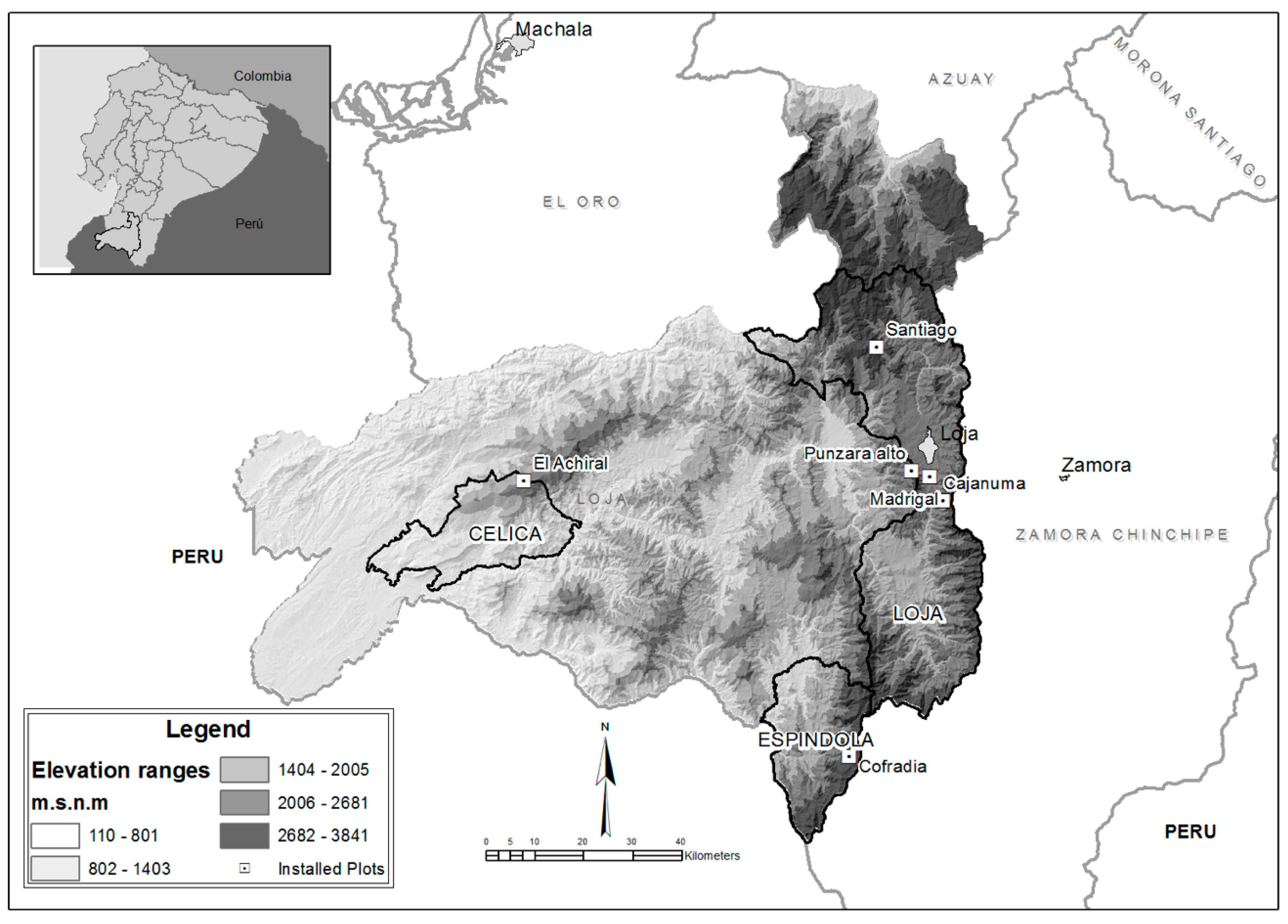
2.1. Study Area

The study was conducted in the province of Loja, located in Southern Ecuador, and the sampling area covered approximately 6000 km2, confirmed by a mosaic of remnants of forests of different sizes embedded in territories dedicated to livestock and agriculture. The distances between plots in each sampling site vary from 1 km (Espíndola) to 0.1 km (Cajanuma, canton Loja). This site is part of a protected area and belongs to a large forest > 500 ha (Podocarpus National Park). Plots are distributed between 2300–2900 m. (Figure 1).

2.2. Sampling Design

One hundred thirty-two plots of 400 m2 were installed following a hierarchical approach. They were organized into three districts (Celica, Espíndola, and Loja), with 6 sample sites (3 in Loja, 1 in Celica and 1 in Espíndola), 44 localities, and three plots for each of the localities (Supplementary Table S1). According to Homeier [24], this area is adequate for surveying trees for comparative purposes in this type of ecosystem. In each plot, the DBH of the trees ≥10 cm was measured, and each individual was identified. The identification of the species was carried out in the field. For the species that could not be identified in the field, a botanical sample was collected for later identification in the Herbarium. Vouchers were included in HUTPL, LOJA, QCA, and QCNE. We followed the catalog of the vascular plants of Ecuador for the nomenclature of the species [25]. Also used the update of the flora of Ecuador [26] and the MOBOT page TROPICOS (www.tropicos.org). To characterize the montane forests of different localities, structural and floristic parameters were calculated using the equations proposed by Madsen & Øllgaard [7] and Magurran [27].
Relative   Diversity ( RD ) = ( species   per   Family Total   species ) 100 Relative   Dominance ( RDm ) = ( Basal   area   per   specie Total   Basal   Area   in   the   group ) 100
Nineteen climate variables available in Worldclim (http://www.worldclim.org; the size of the pixel covers 30 arcseconds or approximately one square kilometer) were used [28]. We also included some additional variables such as the physiographic province, the orogenic geological-landscape, and the lithology of each sector where the plots settle (Supplementary Table S2). The sets of variables were analyzed independently to isolate the effect on diversity and composition, i.e., climate and geomorphological variables versus diversity. Principal component methods are also used for selecting subsets of independent variables for the regression models [29]. The first few components (Supplementary Table S3) were used as predictors in the regression [30,31]. The 19 climatic variables that showed correlation were discarded automatically, leaving 9 main variables (Supplementary Table S4). They were used in principal component analyses (PCA) using the function of R “prcomp” (R Core Team). Finally, we chose the PCA values of the first two main components (Supplementary Table S5).

2.3. Statistical Analysis

2.3.1. Taxonomic Diversity
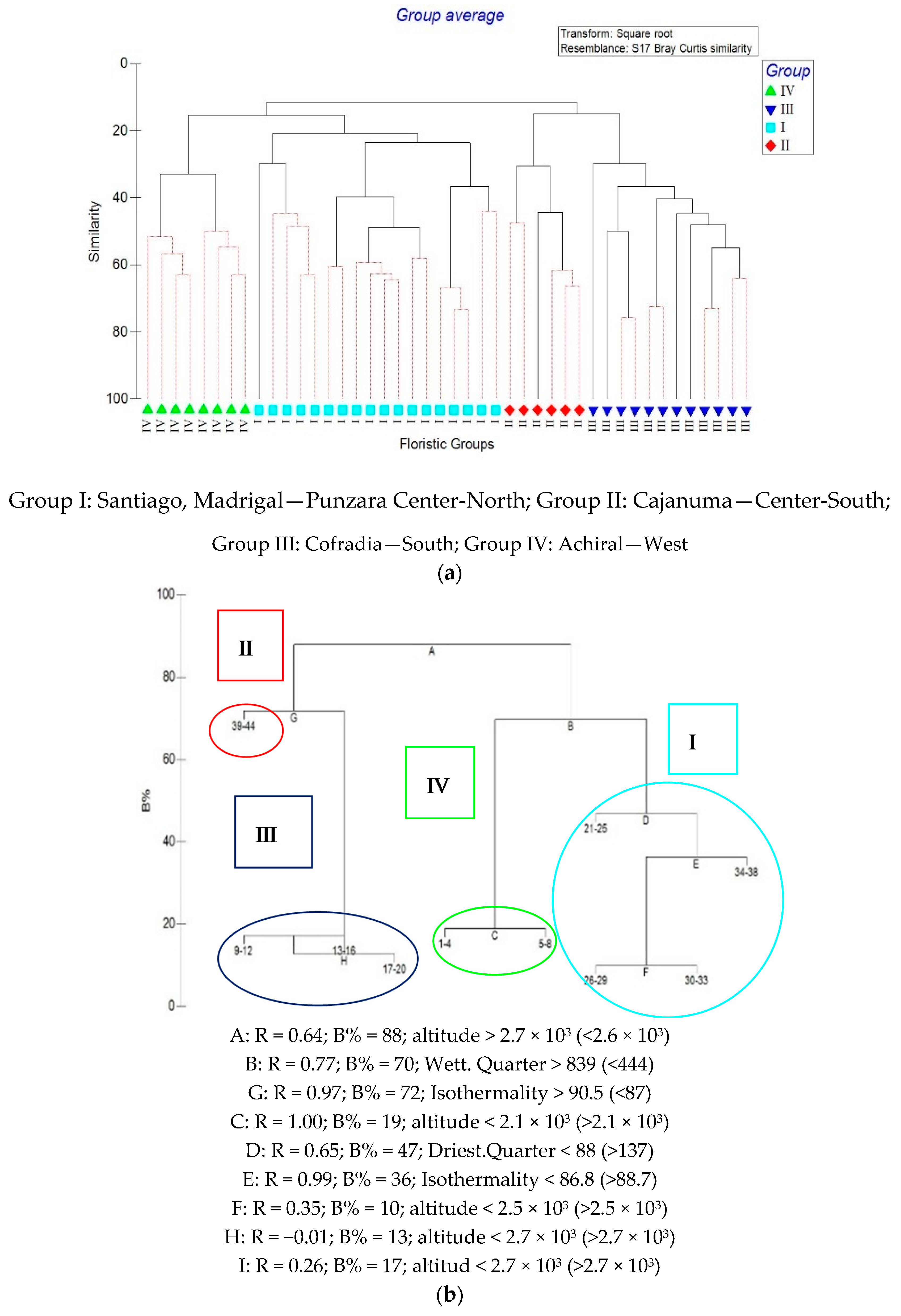
In this study, we combine PCA and the generalized linear models (GLM) to obtain predictive models for Fisher’s alpha diversity calculated at the plot level with other climate variables (rainfall, isothermality, etc.) as predictors. The new variables from PCA are suitable to use as predictors in a regression equation since they remove possible effects of multicollinearity.
To model the total tree diversity (Shannon Index) and evenness, generalized linear models (GLM) were used [32]. The Kruskal-Wallis one-way analysis-of-variance by rank test (H test) was used to determine whether alpha diversity is affected by geomorphological category (physiographic province, great landscape, landscape, and lithology) levels. The basal area was calculated for all trees of each species. To determine differences between the values of the dasometric and floristic variables of each community type (see below), we performed an ANOVA using the aov function. To adjust the model of each of the tests we used the Tukey´s test using the tukey.test function in the software R [33]. When the resulting value of p ≤ 0.05, the difference is significant.

2.3.2. Composition

We used a cluster analysis (complete linkage) to classify all the floristic inventories taken in each plot by using the Bray-Curtis distance as a measure of similarity and transforming the density data (square root) to normalize them. This clustering structure was tested using a profile similarity permutation test (SIMPROF procedure) and a similarity percentage analysis. We used SIMPER similarity percentage analysis to know which species are responsible for the similarity/dissimilarity between floristic groups.
To identify the environmental and geological variables that underlie this classification, we labeled each sample with the environmental variable thresholds obtained after a BIOENV analysis followed by a LINKTREE procedure. These analyses were undertaken using the PRIMER v6 software [34]. Non-metric multidimensional scaling (NMDS) was performed to visualize the main environmental and geomorphological factors that influence the grouping of these forest communities. To calculate the resemblance matrix between plots, the Bray–Curtis dissimilarity distance was used. The results were plotted in an NMDS ordination diagram. Values of species abundance, basal area, trees density, and environmental and geomorphological variables were fitted onto the first two axes of the NMDS ordination. Squared correlation coefficients (r2) and empirical p-values (p) were calculated for these linear fittings. Ordination was performed with the package ‘vegan’ [35] in R software [33].

3. Results

3.1. Alpha Diversity

In the one hundred thirty-two plots analyzed and 4343 individuals sampled, 164 species belonging to 52 botanical families were determined. The five most diverse families were Melastomataceae with 11 species (6.7% of all species); Rubiaceae with 10 species (6.1%) and Asteraceae, Lauraceae and Cunnoniaceae with nine species each (5.5%). There were 22 families that possess a single species (0.6%). Families like Lauraceae, with 502 individuals (11.6%), followed by Melastomataceae with 368 (8.5%) and Clusiaceae with 367 (8.49%), are the most representative families. There were 10 families that have 100–200 individuals (2.5–5.5%); and 24 families had between 10 and 100 individuals (0.3–2.4%). We also detected 14 rare families with 2–9 individuals (0.09–0.2%). The analysis of the composition of the transects resulted in four clearly defined floristic groups. The values of relative diversity and relative dominance of each of them are shown in Table 1 and Table 2.
The total basal area of the sampled individuals reached 157.7 m2. Lauraceae had the highest basal area 19.1 m2 (12.1% of the total), followed by Podocarpaceae with 16.6 m2 (10.5%), Clusiaceae with 13.2 m2 (8.5%), and Cunoniaceae with 10.8 m2 (6.8%). There were twenty-four families with basal areas between 1–10 m2 (0.6–5.6%) and other 24 families with areas of 0.1–1 m2 (0.2 to 0.6%). In each floristic group, there are species with the highest value of the basal area. Some species are characteristic for all groups, and other species are exclusive to each group (Table 2).

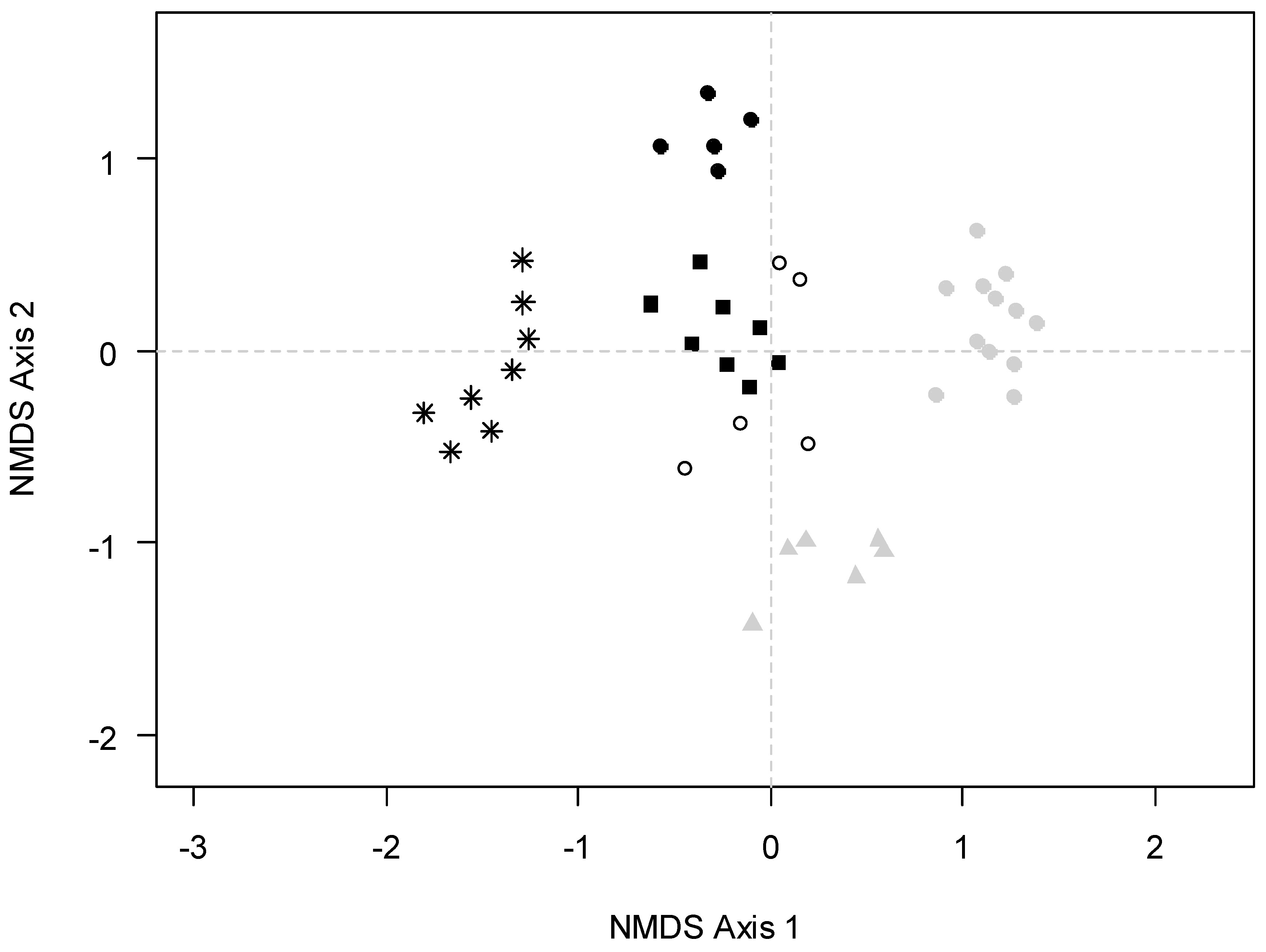
3.2. Species Turnover

The classification based on the SIMPROF test (with permutations) provides four groups (Figure 2). In each cluster node, the percentage of each species which contributes to the differentiation with other nodes was identified. The species that mostly contributed to the dissimilarity between the groups (by SIMPER) were Podocarpus oleifolius, and Podocarpus sprucei, which are typical species of humid montane forests (Group IV). For Guarea kuntiana, A. Juss characterized the floristic Group IV, and the abundance of this species in this group is significant enough to separate it from the rest of the floristic groups. Other species that define the floristic dissimilarity of the groups are Cupania cinerea (Poepp.), Ilex andicola Loes, Weinmannia ovata (Cav.), and Gordonia ourcese (Schrad.) (H. Keng, Table 3). Floristic groups were also strongly influenced by environmental variables and altitude. Groups I and IV are separated from the other groups by altitude (>2700 m). They, in turn, are separated by the influence of the wettest quarter (>839 mm). On the other node, floristic Groups II and III are separated by isothermality (>90.5) representing a high oscillation between the average temperature during the day (Table 4).
The arrangement of the plots clearly indicates an influence of environmental and geomorphologic factors for ordination (Figure 3). Samples of montane forest in Southern Ecuador form four groups: Group I (North–center) consists of the plots on Santiago, Madrigal-Punzara; Group II is comprised of Cajanuma plots (South-central); Group III Cofradía plots (South) and Group IV Achiral plots (West) are also included.
Altitude showed a significant and strong correlation with the NMDS ordination axes, while seasonal temperature and isothermality showed weaker correlations (Table 4). Consistently, altitude, geologic landscape, and lithology factors were relevant predictors of this plant diversity (Table 4). The dissimilarity values indicated high variability of the composition, although there are species that grow indifferently in all groups as Miconia jhanii, Meliosma arenosa, Ilex rupicola, and Meriania tomentosa. We determine 14 families that occur in the four floristic groups. In each group, tree density and relative dominance of the families change along the altitudinal gradient.

3.3. Modeling the Diversity

Principal components (PC1 and PC2) significantly influence the variability of the alpha diversity expressed in the Shannon Index (Table 5). Variables and values included in each component are shown in Supplementary Table S3, and the cumulative values of each component are shown in Supplementary Table S5.
There was a highly significant difference between the “Great Landscape” categories and their alpha-diversity (Kruskal-Wallis, degrees of freedom [df] = 4, χ2 = 20.14, p < 0.001). We compared Fisher’s alpha-diversity index between pairs of geomorphologic landscapes, and “low hills” had significantly higher values compared with the values of “high hills and “dissected mountains” (Wilcoxon rank-sum test W = 126, p < 0.01).
On the other hand, alpha-diversity showed significant differences between “lithology” categories (Kruskal-Wallis, degrees of freedom [df] = 4, χ2 = 23.42, p < 0.001). Then, were compared alpha-diversity values with each level of “lithology”. “Whitish tuffs” showed significantly larger alpha-diversity with respect to “andesitic lavas” (Wilcoxon rank-sum test W = 96, p < 0.001) and “andesitic tuffs” (Wilcoxon rank-sum test, W = 64, p < 0.01).
Along the altitudinal gradient, trees of smaller diameters predominate in all groups (I-IV). Structurally montane forest is heterogeneous, and the number of trees of each diametric class showed significant differences (Table 6), especially in the number of trees in the floristic group II (Cajanuma, South-Central position) where it was higher.

4. Discussion

Our results showed significant changes in the floristic diversity, structure, and composition of the species related to the ecological (altitude) and geomorphological gradients (varied lithology and geological landscapes distributed in a relatively small region) in montane tropical forests. Historically, it is recognized that the elevation of the Andes produced the occurrence of particular environments such as our region, with a great diversity of geological landscapes (mountains dissected, high mountains and low mountains, high and low hills) and becoming a unique region with a huge presence of environmental heterogeneity and complex distribution patterns of diversity and ecosystems [36]. This is one of the reasons behind the adaptation and speciation processes found in tropical zones, mainly being found within the mountain forests found in the tropical Andes and considered as the world center of diversity [37,38,39].
Geomorphological factors related to lithology were the most relevant predictors of alpha diversity of tropical montane forests. Similarly, several studies have confirmed the trend of tropical forests in general, and particularly the mountain forests distribute their species richness driven to certain environmental and topographic gradients [40,41]. Worldwide, mountainous regions show abrupt climate gradients over short distances. The most renowned world centers of diverse vascular plants are found in the mountainous regions of the tropics and sub-humid tropics; these areas have high geodiversity characterized by heterogeneous geology (different lithology) and a high diversity of soils types (a result of the diversity of rocks that make up the region’s lithosphere).
According to Rafiqpoor et al. [42], diversity of the physical environment promotes ecological specialization, and complex ecological landscapes offer greater potential for allopatric speciation. Homeier et al. [41] determined a high correlation between soil nutrients and tree diversity as being related to the availability of these elements (Ca, Mg and pH) which determine or affect corresponding species richness. In addition, the seasonality of precipitation (driest quarter–wettest quarter) appears to be an important factor when defining patterns of diversity and distribution of some species. The tropics are particularly sensitive to the duration of dry periods, particularly species with shallow roots as shrubs and small trees [43]. Similar patterns occur in other latitudes of the planet. For example, alpha diversity decreases as seasonality increases along a latitudinal gradient in tropical areas of India [44].
Theories of distribution patterns of diversity have tried to be explained for centuries. However, concerns about the causes that determine the distribution patterns and the richness of animals and plants persist [44]. According to Kessler et al. [45], for a better understanding of the diversity distribution patterns, these can be studied at different scales. The first is at the regional scale, where the distribution of gamma diversity is determined, including the number of species in broad geographic areas. The second approach includes the determination of alpha diversity and the number of species or local richness in small geographic areas, usually ≤1 ha, as reflected by the approach used in our study. According to Kessler [44] and Willig et al. [46], there are around 100 different hypotheses that try to explain the distribution patterns of diversity which can be grouped into six interrelated areas. In part, these are area availability, climatic variables, energy availability and productivity, historical and evolutionary processes, and neutral theories of stochasticity and population processes such as the “mass effect” and “sink–source” theories.
Regionally, environmental heterogeneity is one of the theories used to explain the high diversity of plants and other taxa [47]. Another critical factor in the distribution of diversity is related to altitude which recognizes four different patterns linked to particular taxonomic groups: The first indicates that diversity decreases with increasing altitude and decreasing particular groups of species, in this particular case small non-winged mammals [48] and bats [49]. Another pattern, called low plateau, indicates that in birds, a maximum of species is achieved at lower elevations, decreasing with increasing altitude [50]. In reptiles, a pattern the low plateau called the intermediate peak (low plateau mid-peak) proposed by McCain [51] is observed. Finally, the pattern called the intermediate peak (mid-peak) proposed by Rahbek [52] shows that the highest expression of diversity occurs in middle elevations, whose pattern starts with a low number of species at lower elevations, reaching the peak of diversity on middle elevations and decreasing when the altitude increases. In Ecuador, the range mountain range crosses the country from North to South, an area in which the ridge is at its lowest point initiating what is known as the “Huancabamba depression” [21]. Under this premise, mountain forests of Southern Ecuador are considered highly diverse, and they are structurally different (supported by a high geomorphological diversity) from other montane forests found at other Ecuadorian latitudes [53].
Locally, montane forestry has been extensively studied in the Eastern slope of the Andes, where the influence of environmental factors results in a high diversity of species, although there are the same types of vegetation in different areas along the mountain range slope [54]. Becking [21] systematized and analyzed the floristic information of 221 sample plots (1030 species) that cover a territory of approximately 10,000 km2 in Loja and Zamora in Southern Ecuador, and their results coincide with the results obtained in our study in relation to altitudinal zoning and montane forest types. However, they did not include montane forests of the western mountain range, which is part of our study. Jørgensen et al. [53] reported the occurrence of plants in low mountain areas (less than 2000 m) without any specific reference to composition or structure.
Our results indicate that the first hierarchical factor in the division of structural and floristic groups is altitude, following by lithology and geologic landscapes; this same factor determines the ordenatión made by Becking [22] and Bussman [19], giving results of altitudinal strips and similar groups in the geographic ranges studied. The results confirm that Lauraceae and Melastomataceae are the most diverse in the four specific floristic groups, although this pattern is very common in Andean forests, which means they are similar in floristic composition to family and genus level, while at the species composition levels they vary considerably. For instance, the floristic group IV (Achiral) located in the Western mountains, unlike the rest of floristic groups, is influenced by the seasonality of dry tropical forests [55] that are nearby. Despite having similar precipitation values with other mountainous areas of the Eastern mountain range, this is concentrated in a relatively short term (three to four months), and the rest of the year is characterized by the lack of rain, while in forests the Eastern precipitation is distributed proportionally throughout the year. The climate process, according to Kessler et al. [45], is linked to distribution patterns of diversity in mountainous areas.
The elevation is the main factor for grouping montane forest plots in four floristic groups, and non-symmetrical shape diversity in these groups is distributed under the concept of diversity mean peak [50]. The climatic factors influence the separation of group IV. The seasonally dry forests that are located in the lower altitude contribute to the composition of the montane forest of group IV (Achiral) structurally and floristically are different from the rest of the forests that appear in the study. Elevation in this area influences the presence of important factors such as fog in certain months [56] and seasonal precipitation, as demonstrated by the previous analysis.
This research confirms the high diversity in the composition and structure of the montane forest in Southern Ecuador. The determined floristic groups are the product of the interaction of climatic, physiographic, and altitudinal conditions, factors that must be present in future forest classifications in the South of Ecuador. The inclusion of other factors apart from the altitude in the ordering of the montane forest shows the variability in the composition and structure and suggests the presence of several communities that can be identified with a deep taxonomic and functional study of the species that compose it. Finally, with respect to the floristic composition of the groups, there are six species that are present in a large part of the transects of all the groups, and they can be considered generalist species, although Podocarpus oleifolius is not present in the transects of Santiago. Contrarily, there are at least 60 species presents in very few transects. In Achiral (Group IV), there are 4 species that do not occur anywhere else. In Group III (Cofradía), there are 10 species that do not occur in any other group. In Group II (Cajanuma), there are 23 exclusive species. In Group I (Santiago-Madrigal-Punzara), there are 23 exclusive species that do not occur in the rest of the groups. According to Becking [21], this specific richness reflects the so-called “ecosystemic singularity” that has also been confirmed in the works of Bussman [9] and Homeier et al. [24].

Supplementary Materials

The following are available online at https://www.mdpi.com/1424-2818/11/3/32/s1, Table S1: Geographical location, altitude and number of plots installed in different study sites; Table S2: Variables used for analysis of the composition and structure of montane forest Southern Ecuador; Table S3: Rotated principal component loadings; Table S4: Pearson correlation matrix of different environmental variables; Table S5: Values of Principal Components Analyses.

Author Contributions

Conceptualization, O.C., Á.B. and A.E.; methodology, O.C., Á.B., A.E.; formal analysis, O.C., Á.B., and P.R.; investigation, O.C., N.C., C.N. and F.T.; data curation, P.R.; writing—original draft preparation, O.C., Á.B., A.E.; writing—review and editing, A.E.

Funding

This research received no external funding.

Acknowledgments

The authors acknowledge the support of the Universidad Técnica Particular de Loja in the development of the field work and analysis of data. We also thank Diego Ramirez, Gonzalo Maldonado, Darwin Carrion, Sergio Cordero, Raul Sinche and Pablo Jaramillo for assistance in dasometric data collection and botanical specimens collecting in different sampling sites.

Conflicts of Interest

The authors declare no conflict of interest.

References

  1. Myers, N.; Mittermeier, R.A.; Mittermeier, C.G.; Da-Fonseca, G.A.; Kent, J. Biodiversity hotspots for conservation priorities. Nature 2000, 403, 853–858. [Google Scholar] [CrossRef] [PubMed]
  2. Brown, A.D.; Kappelle, M. Introducción a los bosques nublados del neotrópico: Una síntesis regional. In Bosques nublados del Neotrópico; Kappelle, M., Brown, A.D., Eds.; Instituto Nacional de Biodiversidad (INBio): Santo Domingo de Heredia, Costa Rica, 2001; pp. 27–40. ISBN 9968-702-50-1. [Google Scholar]
  3. Olson, D.M.; Dinerstein, E. The Global 200: Priority ecoregions for global conservation. Ann. Mo. Bot. Gard. 2002, 89, 199–224. [Google Scholar] [CrossRef]
  4. Mena-Vásconez, P.M. Las áreas protegidas con bosque montano en el Ecuador. In Biodiversity and Conservation of Neotropical Montane Forests; Churchill, P., Balslev, H., Forero, E., Luteyn, J.L., Eds.; The New York Botanical Garden: New York, NY, USA, 1995; pp. 627–635. ISBN 0893273902. [Google Scholar]
  5. Valencia, R. Composition and structure of an Andean forest fragment in Eastern Ecuador. In Biodiversity and Conservation of Neotropical Montane Forests; Churchill, P., Balslev, H., Forero, E., Luteyn, J.L., Eds.; The New York Botanical Garden: New York, NY, USA, 1995; pp. 239–249. ISBN 0893273902. [Google Scholar]
  6. Tapia-Armijos, M.F.; Homeier, J.; Espinosa, C.I.; Leuschner, C.; de la Cruz, M. Deforestation and forest fragmentation in South Ecuador since the 1970s–losing a hotspot of biodiversity. PLoS ONE 2015, 10, e0133701. [Google Scholar] [CrossRef] [PubMed]
  7. Uday, V.; Bussman, R. Floristic distribution of the montane cloud forest at the Tapichalaca Reserve, Canton Palanda, Zamora province. Lyonia 2004, 7, 92–98. [Google Scholar]
  8. Madsen, J.E.; Øllgaard, B. Floristic composition, structure, and dynamics of an upper montane rain forest in Southern Ecuador. Nord. J. Bot. 1994, 14, 403–423. [Google Scholar] [CrossRef]
  9. Bussmann, R.W. The montane forests of Reserva Biologica San Francisco (Zamora-Chinchipe, Ecuador)-vegetation zonation and natural regeneration. Erde 2001, 132, 9–25. [Google Scholar]
  10. Van der Hammen, T. History of the montane forests of the northern Andes. Plant Syst. Evol. 1989, 162, 109–114. [Google Scholar] [CrossRef]
  11. Sodiro, L. Ojeada General Sobre la Vegetación Ecuatoriana; Universidad de Quito: Quito, Ecuador, 1874. [Google Scholar]
  12. Diels, L. Contribuciones al Conocimiento de la Flora y Vegetación de Ecuador; Espinosa, R., Ed.; Anales de la Universidad Central: Quito, Ecuador, 1937. [Google Scholar]
  13. Acosta-Solís, M. Divisiones Fitogeográficas y Formaciones Geobotánicas del Ecuador; Casa de la Cultura ecuatoriana: Quito, Ecuador, 1968. [Google Scholar]
  14. Harling, G. The vegetation types of Ecuador: A brief survey. In Tropical Botany; Larsen, K., Holm-Nielsen, L.B., Eds.; Academic Press: London, UK, 1979; pp. 164–174. ISBN 012437350X. [Google Scholar]
  15. Cañadas-Cruz, L.; Cogez, X.; Lyannaz, J.P.; Ammerman, C.B.; Henry, P.R.; Muñoz, K.A.; Wilson, P.N. El Mapa Bioclimático y Ecológico del Ecuador; Ministerio de Agricultura y Ganadería: Quito, Ecuador, 1983. [Google Scholar]
  16. Ulloa-Ulloa, C.; Jorgensen, P.M. Árboles y Arbustos de los Andes del Ecuador; Department of Systematic Botany: Aarhus, Denmark, 1993. [Google Scholar]
  17. Mosandl, R.; Günter, S.; Stimm, B.; Weber, M. Ecuador suffers the highest deforestation rate in South America. In Gradients in a Tropical Mountain Ecosystem of Ecuador; Beck, E., Bendix, J., Kottke, I., Makeschin, F., Mosandl, R., Eds.; Springer: Berlin, Germany, 2008; pp. 37–40. ISBN 9783540735267. [Google Scholar]
  18. Sierra, R. Propuesta Preliminar de un Sistema de Clasificación de Vegetación para el Ecuador Continental; EcoCiencia: Quito, Ecuador, 1999; ISBN 9789978409435. [Google Scholar]
  19. Bussmann, R.W. Bosques andinos del sur de Ecuador, clasificación, regeneración y uso. Rev. Peruana Biol. 2005, 12, 203–216. [Google Scholar] [CrossRef]
  20. Lozano, P. Los tipos de bosque en el sur de Ecuador. In Botánica Austroecuatoriana–Estudios Sobre los Recursos Vegetales en las Provincias de El Oro, Loja y Zamora Chinchipe; Aguirre, Z., Madsen, J.E., Cotton, E., Balslev, H., Eds.; Abya Yala: Quito, Ecuador, 2002; pp. 29–50. ISBN 9789978222515. [Google Scholar]
  21. Lozano, P.; Bussmann, R.W.; Küppers, M. Diversidad florística del bosque montano en el Occidente del Parque Nacional Podocarpus, Sur del Ecuador y su influencia en la flora pionera en deslizamientos naturales. Rev. Cient. UDO Agríc. 2007, 7, 142–159. [Google Scholar]
  22. Becking, M. Sistema Microregional de Conservación Podocarpus. Tejiendo (Micro) Corredores de Conservación Hacia la Cogestión de una Reserva de la Biosfera Podocarpus-El Cóndor; Programa Podocarpus: Loja, Ecuador, 2004. [Google Scholar]
  23. Lozano, P.; Busmann, R.W.; Küppers, M.; Lozano, D. Natural landslides and pioneer communities in the Mountain Ecosystems of Eastern Podocarpus National Park. Caldasia 2008, 30, 1–19. [Google Scholar] [CrossRef]
  24. Homeier, J.; Breckle, S. Gap-dynamics in a tropical lower montane forest in South Ecuador. In Gradients in a Tropical Mountain Ecosystem of Ecuador; Beck, E., Bendix, J., Kottke, I., Makeschin, F., Mosandl, R., Eds.; Springer: Berlin, Germany, 2008; pp. 311–317. ISBN 9783540735267. [Google Scholar]
  25. Jørgensen, P.M.; León-Yánez, S. Catálogo de las plantas vasculares del Ecuador. Monogr. Syst. Bot. Mo. Bot. Gard. 1999, 75, 1–1181. [Google Scholar]
  26. Ulloa, C.; Neill, D.A. Cinco Años de Adiciones a la Flora del Ecuador 1999–2004; Funbotanica; Universidad Técnica Particular de Loja: Loja, Ecuador, 2005. [Google Scholar]
  27. Magurran, A.E. Why diversity? In Ecological Diversity and Its Measurement; Springer: Dordrecht, The Netherlands, 1988; pp. 1–5. [Google Scholar]
  28. Hijmans, R.J.; Cameron, S.E.; Parra, J.L.; Jones, P.G.; Jarvis, A. Very high resolution interpolated climate surfaces for global land areas. Int. J. Climatol. 2005, 25, 1965–1978. [Google Scholar] [CrossRef] [Green Version]
  29. Sabah, A.A.W.; Charles, S.B.; Salem, M.A.A. Principal component and multiple regression analysis in modeling of ground-level ozone and factors affecting its concentrations. Environ. Model. Softw. 2005, 20, 1263–1271. [Google Scholar] [CrossRef]
  30. Malinowski, R.M. Factor Analysis in Chemistry; Wiley: New York, NY, USA, 1991; ISBN 978-0-471-53009-1. [Google Scholar]
  31. Statheropoulos, M.; Vassiliadis, N.; Pappa, A. Principal component and canonical correlation analysis for examining air pollution and meteorological data. Atmos. Environ. 1998, 32, 1087–1095. [Google Scholar] [CrossRef]
  32. Cayuela, L.; Benayas, J.M.R.; Justel, A.; Salas-Rey, J. Modelling tree diversity in a highly fragmented tropical montane landscape. Glob. Ecol. Biogeogr. 2006, 15, 602–613. [Google Scholar] [CrossRef]
  33. R Development Core Team. A Language and Environment for Statistical Computing; R Foundation for Statistical Computing: Vienna, Austria, 2013; ISBN 3-900051-07-0. [Google Scholar]
  34. Clarke, K.R.; Gorley, R.N. PRIMER v6: User Manual/Tutorial; Plymouth Routines in Multivariate Ecological Research: Plymouth, MA, USA; Primer-E Ltd.: Auckland, New Zealand, 2006. [Google Scholar]
  35. Oksanen, J.; Blanchet, F.G.; Kindt, R.; Legendre, P.; Minchin, P.R.; O’Hara, R.B.; Oksanen, M.J. Package ‘vegan’. Community Ecology Package. Version, 2(9). 2013. Available online: https://cran.r-project.org/web/packages/vegan/vegan.pdf (accessed on 12 October 2018).
  36. Josse, C.; Navarro, G.; Comer, P.; Evans, R.; Faber-Langendoen, D.; Fellows, M.; Kittel, G.; Menard, S.; Pyne, M.; Teague, J. Ecological Systems of Latin America and the Caribbean: A Working Classification of Terrestrial Systems; NatureServe: Arlington, VA, USA, 2003. [Google Scholar]
  37. Churchill, S.P.; Balslev, H.; Forero, E.; Luteyn, J.L. Biodiversity and Conservation of Neotropical Montane Forests; New York Botanical Garden: New York, NY, USA, 1995. [Google Scholar]
  38. Bush, M.B.; Hanselman, J.A.; Hooghiemstra, H. Andean montane forests and climate change. In Tropical Rainforest Response to Climatic Change; Bush, M.B., Flenley, J., Eds.; Springer: Berlin/Heidelberg, Germany, 2007; pp. 59–79. ISBN 978-3-642-05383-2. [Google Scholar]
  39. Antonelli, A.; Sanmartín, I. Why are there so many plant species in the Neotropics? Taxon 2011, 60, 403–414. [Google Scholar] [CrossRef]
  40. Givnish, T.J. Altitudinal gradients in tropical forest composition, structure, and diversity in the Sierra de Manantlán. J. Ecol. 1998, 86, 999–1020. [Google Scholar]
  41. Homeier, J.; Breckle, S.W.; Günter, S.; Rollenbeck, R.T.; Leuschner, C. Tree Diversity, Forest Structure and Productivity along Altitudinal and Topographical Gradients in a Species-Rich Ecuadorian Montane Rain Forest. Biotropica 2010, 42, 140–148. [Google Scholar] [CrossRef]
  42. Rafiqpoor, D.; Kier, G.; Kreft, H. Global centers of vascular plant diversity. Nova Acta Leopoldina 2005, 92, 61–83. [Google Scholar]
  43. Condit, R.; Hubbell, S.P.; Foster, R.B. Mortality rates of 205 neotropical tree and shrub species and the impact of a severe drought. Ecol. Monogr. 1995, 65, 419–439. [Google Scholar] [CrossRef]
  44. Kessler, M. The impact of population processes on patterns of species richness: Lessons from elevational gradients. Basic Appl. Ecol. 2009, 10, 295–299. [Google Scholar] [CrossRef] [Green Version]
  45. Kessler, M.; Kluge, J.; Hemp, A.; Ohlemüller, R. A global comparative analysis of elevational species richness patterns of ferns. Glob. Ecol. Biogeogr. 2011, 20, 868–880. [Google Scholar] [CrossRef]
  46. Willig, M.R.; Kaufman, D.M.; Stevens, R.D. Latitudinal gradients of biodiversity: Pattern, process, scale, and synthesis. Annu. Rev. Ecol. Evol. Syst. 2003, 34, 273–309. [Google Scholar] [CrossRef]
  47. Kreft, H.; Jetz, W. Global patterns and determinants of vascular plant diversity. Proc. Natl. Acad. Sci. Biol. 2007, 104, 5925–5930. [Google Scholar] [CrossRef] [PubMed] [Green Version]
  48. McCain, C.M. Elevational gradients in diversity of small mammals. Ecology 2005, 86, 366–372. [Google Scholar] [CrossRef]
  49. McCain, C.M. Could temperature and water availability drive elevational species richness patterns? A global case study for bats. Glob. Ecol. Biogeogr. 2007, 16, 1–13. [Google Scholar] [CrossRef]
  50. McCain, C.M. Global analysis of bird elevational diversity. Glob. Ecol. Biogeogr. 2009, 18, 346–360. [Google Scholar] [CrossRef]
  51. McCain, C.M. Global analysis of reptile elevational diversity. Glob. Ecol. Biogeogr. 2010, 4, 541–553. [Google Scholar] [CrossRef]
  52. Rahbek, C. The role of spatial scale and the perception of large-scale species-richness patterns. Ecol. Lett. 2005, 8, 224–239. [Google Scholar] [CrossRef]
  53. Jørgensen, P.M.; Ulloa-Ulloa, C.; Madsen, J.E.; Valencia, R. A floristic analysis of the high Andes of Ecuador. In Biodiversity and Conservation of Neotropical Montane Forests; Churchill, S.P., Balslev, H., Forero, E., Luteyn, J.L., Eds.; New York Bot. Gard: New York, NY, USA, 1995; pp. 221–238. [Google Scholar]
  54. Matteucci, S.D.; Colma, A. Metodología para el Estudio de la Vegetación; Secretaría General de la Organización de los Estados Americanos, Programa Regional de Desarrollo Científico y Tecnológico: Washington, DC, USA, 1982. [Google Scholar]
  55. Espinosa, C.I.; De la Cruz, M.; Luzuriaga, A.L.; Escudero, A. Bosques tropicales secos de la región Pacífico Ecuatorial: Diversidad, estructura, funcionamiento e implicaciones para la conservación. Ecosistemas 2012, 21, 1–2. [Google Scholar]
  56. Richter, M.; Moreira-Muñoz, A. Heterogeneidad climática y diversidad de la vegetación en el sur de Ecuador: Un método de fitoindicación. Rev. Peruana Biol. 2005, 12, 217–238. [Google Scholar]
Figure 1. Map location of sampling plots.
Diversity 11 00032 g001
Figure 2. (a) Cluster based on floristic similarity using the Bray-Curtis measure (SIMPROF) and (b) Dendrogram (LINKTREE) grouping plots based on environment variables and the altitude of montane forests in Southern Ecuador. Use of the same color represents the same floristic group.
Diversity 11 00032 g002
Figure 3. Non-metric multidimensional scaling analysis of species composition for the samples (plots) in the studied montane rain forests. Santiago forest (white circle), Punzara forest (black circle), and Madrigal forest (black square) conform to Group I. Cajanuma forests (gray triangle) represent Group II, Cofradia forests (gray circle) represent Group III, and Achiral forests (star) conform to Group IV.
Diversity 11 00032 g003
Table 1. Families with more species of the total determined (relative diversity) in the four determined floristic groups (NMDS) of the montane forest in our study.
GroupsFamilies# SpeciesRelative Diversity
IMELASTOMATACEAE109.01
LAURACEAE87.21
ASTERACEAE65.41
CUNNONIACEAE65.41
RUBIACEAE65.41
IIAQUIFOLIACEAE69.38
MELASTOMATACEAE69.38
CUNNONIACEAE57.81
LAURACEAE57.81
SYMPLOCACEAE57.81
IIIAQUIFOLIACEAE69.38
MELASTOMATACEAE69.38
CUNNONIACEAE57.81
LAURACEAE57.81
SYMPLOCACEAE57.81
IVLAURACEAE611.11
EUPHORBIACEAE59.26
MYRTACEAE47.41
ASTERACEAE35.56
MELASTOMATACEAE35.56
Table 2. Species with greater basal area in each floristic group.
GroupsSpeciesBasal Area (m2)Relative Dominance
ISchefflera ferruginea (Kunth) Harms48.1
Critoniopsis pycnantha (Benth.) H. Rob.2.55.1
Oreopanax eriocephalus Harms2.24.5
Nectandra reticulata (Ruiz & Pav.) Mez2.24.5
Clusia alata Triana & Planch.1.63.3
IIPrumnopitys montana (Humb. & Bonpl.) Laub.1.88.6
Persea ferruginea Kunth1.46.4
Clusia alata Triana & Planch.1.36.2
Gordonia fruticosa (Schrad.) H. Keng.1.36
Weinmannia ovata Cav.1.35.9
IIIPodocarpus oleifolius D. Don ex Lamb.10.117.4
Clusia alata Triana & Planch.4.17.1
Persea ferruginea Kunth3.76.3
Citronella sp.3.56
Podocarpus sprucei Parlatore3.45.9
IVGuarea kunthiana A. Juss.2.68.8
Miconia jahnii Pittier2.37.9
Endlicheria sp.2.17
Nectandra laurel Ness1.86.1
Myrcianthes discolor (Kunth) McVaugh.1.86
Table 3. Floristic dissimilarity values between groups and species that contribute with their presence and abundance to the floristic difference.
Groups IV & IIIAverage Dissimilarity = 95.40
Group IVGroup III
SpeciesAv.AbundAv.AbundAv.DissDiss/SDContrib%Cum.%
Podocarpus oleifolius D. Don ex Lamb.03.063.652.983.833.83
Miconia jahnii Pittier2.980.143.412.663.587.41
Guarea kunthiana A. Juss.2.6203.12.513.2410.65
Clusia latipes Triana & Planch.02.192.611.712.7413.39
Aniba muca (Ruiz&Pav) Mez2.250.222.591.42.7216.11
Groups IV & IAverage dissimilarity = 84.56
Group IVGroup I
Guarea kunthiana A. Juss.2.620.212.851.963.373.37
Miconia jahnii Pittier2.981.152.431.352.876.25
Aniba muca (Ruiz&Pav) Mez2.250.572.391.272.829.07
Cupania cinerea Poepp.1.7202.130.882.5211.6
Nectandra laurel Ness1.650.91.871.092.2113.8
Groups III & IAverage dissimilarity = 86.22
Group IIIGroup I
Podocarpus oleifolius D. Don ex Lamb.3.060.223.352.253.883.88
Clusia latipes Triana & Planch.2.190.232.361.482.746.62
Ilex andicola Loes2.090.112.351.612.729.34
Podocarpus sprucei Parlatore1.9802.282.152.6411.99
Citronella sp.1.9302.181.182.5314.51
Groups IV & IIAverage dissimilarity = 91.53
Group IVGroup II
Weinmannia ovata Cav.02.752.831.593.093.09
Guarea kunthiana A. Juss.2.6202.762.393.016.1
Aniba muca (Ruiz&Pav) Mez2.2502.391.42.618.72
Persea ferruginea Kunth02.22.311.222.5311.24
Gordonia fruticosa02.192.242.252.4513.69
Groups III & IIAverage dissimilarity = 85.12
Group IIIGroup II
Weinmannia ovata Cav.02.752.791.593.283.28
Miconia jahnii Pittier0.142.612.551.92.996.27
Gordonia fruticosa02.192.212.252.68.87
Clusia alata Triana & Planch.1.642.072.181.312.5711.43
Ilex andicola Loes2.0902.181.72.5613.99
Groups I & IIAverage dissimilarity = 85.28
Group IGroup II
Weinmannia ovata Cav.02.752.761.543.233.23
Gordonia fruticosa (Schrad.)H.Keng02.192.182.152.565.79
Clusia alata Triana & Planch.1.112.072.11.152.468.25
Weinmannia elliptica Kunth0.062.072.011.512.3610.61
Miconia jahnii Pittier1.152.611.991.442.3312.94
Table 4. Significant variables affecting the grouping of montane forest in Southern Ecuador.
Vectors
NMDS1NMDS2r2p-Value
Altitude0.882−0.4690.7101<0.0001
Temperature Season0.730−0.6860.17130.0199
Isothermality0.4670.8840.24620.0059
Factors
West Cordillera−1.458−0.105
East Cordillera0.3240.023
Physiographic province 0.3924<0.0001
Denudative0.58560.128
Fluvial Erosional−0.488−0.106
Great landscape 0.2474<0.0001
Low Hills−0.25030.093
High Hills0.71270.436
High Mountain0.2963−1.111
Low Mountain−0.0453−0.131
Dissected Mountain−1.458−0.105
Landscape 0.7057<0.0001
Andesitic collade1.1420.151
Intrusive−0.045−0.131
Metamorphic0.016−0.096
Andesitic Tuffs−1.458−0.105
Whitish Tuffs−0.2500.093
Litology 0.6351<0.0001
Table 5. Generalized linear models of total tree diversity (Shannon Index) with two principal components (PC1 and PC2), respectively.
MODELEstimateStd. Errort ValuePr(>|t|)
Intercept0.00852170.000899.479<0.001 ***
PC 1−0.00123920.00028−4.294<0.001 ***
PC 20.00276770.000893.095<0.01 *
Signif. codes: *** 0–0.001; * ≥0.01 AIC: 244.85.
Table 6. Structural parameters and diversity of montane forest in Southern Ecuador. The mean value ± SD is shown; different letters show significant differences (p ≤ 0.05).
ParametersG1
(Santiago-Punzara-Madrigal)
G2
(Cajanuma)
G3
(Cofradía)
G4
(Achiral)
Shannon Diversity Index
(/400 m2)
28.9 ± 8.6a30 ± 4.51b21.1 ± 4.3a22.8 ± 2.3a
Species Tree Richness/400 m2.6 ± 0.4a2.58 ± 0.22a2.44 ± 0.34a2.88 ± 0.12b
Trees/400 m (>10 cm DAP)86.1 ± 28.9a127.3 ± 40.9b112 ± 15.3a96.7 ± 17.9a
Basal Area (>10 cm DAP)2.7 ± 0.9a3.6 ± 1.2a4.9 ± 1.8b3.7 ± 0.6a

