Heterogeneous Polymer Dynamics Explored Using Static 1H NMR Spectra


Department of Organic Materials Science, Sandia National Laboratories, Albuquerque, NM 87185, USA
*
Author to whom correspondence should be addressed.
Int. J. Mol. Sci. 2020, 21(15), 5176; https://doi.org/10.3390/ijms21155176
Submission received: 17 June 2020
/
Revised: 8 July 2020
/
Accepted: 8 July 2020
/
Published: 22 July 2020
(This article belongs to the Special Issue NMR Characterization of Amorphous and Disordered Materials)
Abstract
:NMR spectroscopy continues to provide important molecular level details of dynamics in different polymer materials, ranging from rubbers to highly crosslinked composites. It has been argued that thermoset polymers containing dynamic and chemical heterogeneities can be fully cured at temperatures well below the final glass transition temperature (Tg). In this paper, we described the use of static solid-state 1H NMR spectroscopy to measure the activation of different chain dynamics as a function of temperature. Near Tg, increasing polymer segmental chain fluctuations lead to dynamic averaging of the local homonuclear proton-proton (1H-1H) dipolar couplings, as reflected in the reduction of the NMR line shape second moment (M2) when motions are faster than the magnitude of the dipolar coupling. In general, for polymer systems, distributions in the dynamic correlation times are commonly expected. To help identify the limitations and pitfalls of M2 analyses, the impact of activation energy or, equivalently, correlation time distributions, on the analysis of 1H NMR M2 temperature variations is explored. It is shown by using normalized reference curves that the distributions in dynamic activation energies can be measured from the M2 temperature behavior. An example of the M2 analysis for a series of thermosetting polymers with systematically varied dynamic heterogeneity is presented and discussed.
1. Introduction
Solid-state NMR spectroscopy remains an important tool for the characterization of the structure and dynamics in a wide range of materials [1,2,3,4,5]. Improvements in magic angle spinning (MAS) spinning speeds; advances in heteronuclear, multiple dimensional, and multiple quantum NMR pulse sequences; plus the sensitivity gains realized from dynamic nuclear polarization (DNP) methods continue to impact the use of NMR to probe a variety of different material phenomena. While many of these advances help resolve additional molecular level details, there is a corresponding increase in the complexity of implementation. One of the oldest and, perhaps, simplest methods for the analysis of NMR spectra involves measuring the second moment (M2) of the line shapes as a function of the temperature or composition [6,7] and has proven to be indispensable in characterizing dynamics and local structures in amorphous and disordered materials. Static (non-spinning) NMR line shapes are broadened by homonuclear and heteronuclear dipolar couplings between different nuclei, quadrupolar couplings (for spin I > ½), chemical shielding anisotropy, or chemical shift dispersions, thus providing a handle to probe local structures and dynamics. For example, 7Li, 23Na, 31P, and 133Cs NMR M2 results have been reported for glasses in analyses of structures and ion dynamics [8,9,10,11,12], as well as 1H NMR M2 studies of dynamics, miscibility, and chain orientations in polymers [13,14,15,16,17,18,19,20]. While static NMR is hampered by low spectral resolution, it does benefit from being sensitive to local motions on the order of the line width and can be employed over very wide temperatures ranges.
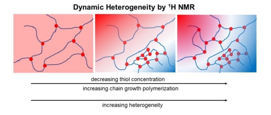
Our group has recently explored the impact of dynamic heterogeneity on polymer thermosets that can be cured (polymerized) at temperatures well below the final observed glass transition temperature Tg [20]. Here dynamic heterogeneity refers to the existence of regions within the thermoset where the polymer chain segment fluctuations have different correlation times or exhibit differences in the widths of the correlation time distributions. NMR proves to be a powerful tool to probe these heterogeneities at the molecular level. Thiol–ene polymerizations combine both chain-growth and step-growth mechanisms, enabling the systematic variation of dynamic heterogeneity through the stoichiometry of the polymerization mixture [21,22,23,24,25,26,27,28], which can be used to control the relationship between the cure temperature and the final Tg. We prepared a series of high-Tg materials, in which the heterogeneity was modulated by the reacting mixtures of the aromatic monomer 1,3,5-benzenetrithiol (BTT) and tricyclodecane dimethanol diacrylate (TCDDA) with differing ratios of the reactive functional groups. These mixtures are identified by R = (SH)0/(C=C)0, where (SH)0 and (C= C)0 were the initial concentrations of the thiol and acrylate functionality, respectively. The polymer mixtures were ultraviolet (UV) cured in the presence of the photo-initiator p-xylylene bis(N,N-diethyldithiocarbamate) (XDT), as shown in Scheme 1. The resulting thermosets incorporate both the chain-growth homo-polymerization of the acrylate groups and step-growth co-polymerization of the thiol and acrylate groups, which yield comparatively heterogeneous and homogeneous networks, respectively. Chain-growth thermosets are described as containing a nonuniform distribution of crosslinks at the nanoscale [29], which should be reflected in the nonuniform correlation time (or relaxation rates) distributions for the polymer chain fluctuations. By decreasing R (lower thiol concentration), the polymerization is biased towards the chain-growth mechanism and is expected to increase the heterogeneity in the local crosslink density and, correspondingly, an increase in the distribution of the polymer chain relaxation rates. Additional physical characterizations of these TCDDA-BTT networks have previously been reported [20]. In that study, we reported the temperature variation of the second moment (M2) of the 1H NMR spectral line shape, along with qualitative arguments for increased dynamic heterogeneity in low R value networks. In the current study, we present an analysis of how dynamic distributions or dynamic heterogeneity are reflected in both the M2 temperature variation and the estimated polymer chain correlation times (τc).
2. Results and Discussion
Static solid-state 1H NMR spectra for the UV-cured BTT-TCDDA networks as a function of temperature and R are shown in Figure 1. At 233 K (−40 °C), a single unresolved broad resonance having a full width at a half-maximum line width of~50 kHz is observed for all R ratios. This broad resonance originates from the strong homonuclear 1H-1H dipolar couplings present in these rigid, glassy polymers. At these low temperatures, the local polymer chain dynamics are slow compared to the timescale of the dipolar interaction (i.e., 1/τc << 2π(M2)1/2, where τc is the correlation time of the chain fluctuations and (M2)1/2 is related to the spectral line width). Note, for the solid-state 1H NMR spectra at low temperatures, there are no narrow spectral components overlapping the broad resonances. This lack of a narrow resonance clearly shows that highly mobile polymer fractions (1/τc >> 2π(M2)1/2) from comparatively low crosslink density regions are not present. Another way to describe this is that, if there are low crosslink density regions, they must have similar dynamic responses to the rest of the network when well below the Tg. With increasing temperatures, additional polymer dynamics are activated, leading to the motional averaging of the dipolar coupling (1/τc~2π(M2)1/2) and gradual narrowing of the NMR line resonance. This motional averaging dramatically increases near the Tg, where the rate and magnitude of the polymer chain fluctuations (α-relaxation) become large enough to ultimately produce the fully dynamically averaged narrow line shapes observed at high temperatures (Figure 1). With the decreasing R, the temperature at which the α-relaxation becomes activated increases and mirrors the change observed in the dynamic mechanical analysis (DMA) (Supplementary Materials Figure S1). For the BTT-TCDDA networks discussed here, the dynamic heterogeneities (i.e., a distinct mixture of narrow and broad resonances) observed in the 1H NMR line shape as a function of R near the Tg are not as pronounced as those previously noted in related networks [20] and most likely reflect the differences in the UV light source intensity employed and the actual sample temperature during the cure process.
While it is common during the analysis of static 1H NMR line shapes to simply deconvolute the resonance into mobile and immobile fractions, polymer chain dynamics realistically involve a distribution of motional rates, leading to a complex superposition of different motionally averaged line shapes. Here, we describe an analysis of M2 calculated using the spectral intensity at frequency ω over the entire line shape for each NMR spectrum using (see Appendix A for details):
![Ijms 21 05176 i001]()

The temperature variation of the 1H NMR M2 for BTT-TCDDA networks as a function of R is shown in Figure 2a. In the low temperature regime M2 for R = 0.00 and 0.09, the networks are similar but are significantly larger than the M2 for R = 0.47 and 0.32, while R = 0.19 is intermediate between these extremes. The larger M2 at a low temperature (increased magnitude of the 1H-1H dipolar coupling) may result from multiple factors. The first possibility is that the TCDDA component has an increased intra- or intermolecular dipolar coupling (higher intra- or intermolecular proton density) than the BTT and that higher TCDDA concentrations (decreasing R) will therefore increase the M2. The proton density for the pure monomers is estimated to be 0.087 moles H/cm3 and 0.047 moles H/cm3 for BTT and TCDDA, respectively, supporting the argument that proton density increases with decreasing R. While the M2 has not been theoretically calculated for the cured TCDDA-BTT polymers, as the network structures are not known, we argue that the 100-kHz2 differences in the M2 at 233 K cannot be fully explained by the compositional change. The most reasonable explanation is that, at this temperature, the TCCDA rich compositions have dynamics that are more representative of the rigid glassy state, since, at 233 K, the temperature is further from their respective Tg values. To support this, the M2 is plotted with respect to the scaled temperature (T-Tg)/Tg, as shown in Figure 2b, which reveals that all compositions trend to the same M2 limit. Due to probe hardware limitations, we were not able to investigate temperatures below 233K, preventing us from reaching the rigid lattice limit for all compositions.
Between 233 K and 400 K, there is a gradual decrease in the M2 with the increasing temperature (Figure 2a), which is attributed to the β-relaxation process involving local, noncooperative dynamics in the BTT-TCDDA network. The M2 temperature variation for this β-relaxation process is similar for all compositions. As the temperature is further increased through a given Tg, the respective M2 rapidly decreases due to dynamic averaging as the polymer chain motions become faster and more dominant (α-relaxation), until finally reaching the rubbery plateau regions for T > Tg. The expansion of the M2 temperature variation for the BTT-TCDDA networks at reduced temperatures near (T-Tg)/Tg~0 (Figure 2c) reveals distinctly different dynamics, which we will attribute to differences in the activation energy (and corresponding correlation times) for the polymer chain motions in subsequent sections. Additional NMR relaxation experiments, including spin lattice relaxation (T1) and spin-spin relaxation (T2), were not pursued for the current study due to the desire to match the NMR heating/cooling rates to the heating/cooling rates of the DMA analysis as closely as possible.
2.1. Impact of Activation Energy on M2
To extract additional information regarding polymer chain dynamics from the 1H NMR spectra, it is instructive to model the effect of different variables on the M2 behavior. Figure 3 shows simulations of the M2 temperature variation for varying activation energies (Ea) of the dynamic process leading to the motional averaging. The temperature behavior of the M2 is defined using Equation (A5) (additional discussion provided in the Appendix A), where we have assumed an Arrhenius behavior for the correlation times τc using:
where τ0 is the pre-exponential correlation time, Ea the activation energy, and Rgas is the gas constant. The pre-exponential term was fixed at τ0 = 0.5905 ns for all simulations, unless otherwise noted. This τ0 value is in the middle of the range experimentally determined (see Table 1 and later discussion). An example of the simulated M2 variations for changing τ0 is shown in Figure S2. A more complicated non-Arrhenius temperature behavior of τc, such as the Vogel-Fulcher-Tammann (VFT) relationship [30,31,32], could also be considered. As expected, the transition from the rigid lattice M2 limit to the fully motionally averaged M2 occurs at higher temperatures with increasing Ea. The M2 temperature variations for this range of Ea overlap when scaled to the reduced temperature (T-Tg)/Tg, as shown in Figure 3b, with this scaling behavior being well-known in the analysis of polymer relaxation processes [33,34,35].
2.2. Distributions in Dynamic Rates
In amorphous polymers, it is expected that the dynamics include a distribution of chain relaxation correlation times, as previously included in NMR line shapes and relaxation time analyses [36,37,38]. Since a variation in Ea moves the temperature at which the Tg transition is observed (Figure 3), the presence of a distribution of activation energies will therefore impact the M2 temperature variation. As an example, Figure 4a shows the simulated M2 variation with the introduction of a Gaussian distribution of the log mean correlation time τ * or, equivalently, a Gaussian distribution of Ea (see Equation (A8)) with different standard deviations σ. Examples of these Gaussian distributions are shown in Figure S3. The results are labeled as a function of σ(Ea) for direct comparison to Figure 3. With the increasing σ, the rate of change of the M2 with the temperature is reduced, with the width of the Tg transition broadened, and is reminiscent of the DMA results shown in Figure S1. This broadening behavior results from the increasing fraction of polymer chains having either slower (higher Ea) or faster (lower Ea) relaxation rates. For a Gaussian distribution, the M2 intensities at different σ are equivalent at the same Tg temperature (here, 442 K), because the mean Ea is independent of σ for a symmetric distribution.
Another distribution commonly employed to describe polymer relaxation is the Davidson-Cole (DC) relationship [39] defined by Equation (A9), with an example of the distribution shown in Figure S3. The temperature variation of the M2 as a function of the increasing distribution breadth (decreasing ε) is shown in Figure 4b. The behavior is distinct from that observed for a Gaussian distribution. In the DC distribution model, the M2 transition is broadened with a decreasing ε for temperatures below the original Tg (transition temperature). This broadening results from a larger fraction of polymer chain motions being activated at lower temperatures (1/τc~2π(M2)1/2) due to the increased concentration of regions (e.g., defects, reduced crosslink density, etc.) having reduced Ea values. For temperatures above the original Tg transition, there is limited impact on the M2 behavior, because the DC distribution (Equation (A9)) is described by the maximum correlation time above which the probability of the slower dynamic processes vanishes. The asymmetry of the DC probability shifts the observed Tg (defined here as the midpoint in the M2 transition) to lower temperatures. The variations in the M2 as a function of the reduced temperatures for systems with either a Gaussian or a DC distribution are shown in Figure 5a,b, respectively. For small distribution widths, the M2 temperature behavior is very similar and only begins to deviate for large distributions.
The comparison of the M2 temperature variation between different network compositions may be complicated by differences in both the Ea (different Tg values) and distribution widths. This issue is explored in Figure 6 for the Gaussian and DC distributions. The M2 temperature behavior (Figure 6a,b) does not readily allow differences in the distribution to be realized, but, by simply mapping the M2 behavior to a reduced temperature scale, the presence of the distributions is clear, regardless of the different Ea (Figure 6c,d). The M2 behavior is related to the relative magnitude of σ with respect to the Ea, but for similar ranges of the Ea, the M2 curves overlap well for a given value of σ. Therefore, by plotting the M2 with respect to reduced temperatures, it should be possible to experimentally measure distributions of polymer chain dynamics near Tg from static solid-state 1H NMR experiments.
2.3. Multiple Dynamic Processes
The impact of multiple dynamic processes on the M2 temperature behavior has previously been discussed by several authors [40,41,42,43,44,45,46,47,48]. For two noncorrelated dynamic processes, the M2 behavior is defined by Equation (A10). An example is shown in Figure 7 involving a slow dynamic process at lower temperatures (β-relaxation), defined by the activation energy Ea(1), and a second dynamic process (α-relaxation, glass transition) at higher temperatures defined by the activation energy Ea(2). In these simulations, it is very easy to distinguish the two separate dynamic averaging transitions (Figure 7a) by the two-step features that are predicted, consistent with the work of Bilski and coworkers [41]. The addition of Ea(1) distributions to the β-relaxation transition (Figure 7b) begins to obscure the reduction step in the M2 resulting from this dynamic process. This M2 behavior is reminiscent of the M2 variation seen before the main Tg transition for the BTT-TCDDA networks (Figure 2). We were unable to reach the low temperature rigid lattice M2 plateau prior to β-relaxation due to the experimental limitations. The distinct M2 step has only rarely been observed for thermosets (see Figure 4 in Reference [19]) consistent with the presence of significant distributions for β-relaxation dynamics. These limitations result in the poorly constrained fitting of the initial β-relaxation process, such that we will concentrate only on the larger α-relaxation (glass transition) region at higher temperatures.
2.4. Distributions in BTT-TCDDA Networks
By considering the M2 variation near Tg and utilizing the reduced temperature, reference curves for the M2 variation with either a Gaussian or a DC distribution were developed, as shown in Figure 8a,b, respectively. With increasing distribution widths (increasing σ or decreasing ε), the M2 variation across the glass transition region is broadened. For the Gaussian distribution, only σ changes on the order of ±1 are distinguishable, while, for the DC distributions, ε variations on the order of ±0.05 can be distinguished, except between ε = 0.5 and 1.0, where the impact on the M2 variation is minimal. The overall M2 behavior in the reference curves is similar for the Gaussian and DC distribution models, but they become slightly more distinct for very large distribution widths. For the current study, the differences in the distribution widths as a function of the composition R are not large enough for the M2 analysis to reliably distinguish between the Gaussian and DC distribution models.
The M2 temperature variation for the BTT-TCDDA networks are plotted in Figure 8c,d on the Gaussian and DC distribution reference curves. There is clearly an increase in the distribution with the decreasing R, and assuming a Gaussian distribution, we can assign σ accordingly. Starting from σ < 1 for R = 0.47 and then increasing to σ = 2 for R = 0.19, σ = 3 to 4 for R = 0.09 and σ = 5 for R = 0.0. The M2 response for the R = 0.47 and R = 0.32 curves were not distinguishable and suggest that the distribution change between these two R compositions is within one sigma. Similarly, assuming a DC distribution, ε > 0.4 for the R = 0.47 and R = 0.32 compositions (recall that, between ε = 0.5 and 1.0, the reference curves are indistinguishable), then the distribution width increases with ε = 0.35 for R = 0.19, ε = 0.3 for R = 0.09, and to ε = 0.25 for the R = 0.0 network. It is also important to note that the M2 behavior for the R = 0.0 BTT-TCDDA network is not symmetric around Tg, which we have attributed to the degradation of this material at the very high temperatures (> 600 K or > 325 °C) achieved in the variable temperature experiments for this composition, and produced irreversible changes in the M2 behaviors. These results are summarized in Table 1 and reveal that, in the BTT-TCDDA networks, the distribution in Ea (and, correspondingly, τc) increases with the decreasing R. This is consistent with the picture of increased heterogeneous dynamics due to the chain-growth mechanism being dominant at high acrylate concentrations.
2.5. Dynamic Correlation Times
While the reference curves presented above allowed the distribution in activation energies or correlation times to be assessed, we also wanted to explore the impact distributions have on the Arrhenius analysis that had assumed a single correlation time when analyzing the M2 temperature behavior. An “effective” correlation time, τeff, to describe the polymer chain fluctuations near the Tg was determined using Equation (A6) (additional discussion is provided in the Appendix A) [6,7,19,20,49]. Activation energies were then estimated assuming the Arrhenius behavior of τeff in the high temperature limit. The low temperature plateau shows an invariant τeff and is an artifact of the dynamics not being fast enough at these low temperatures to average the dipolar coupling (i.e., very slow motions are not probed by the 1H M2). For a Gaussian distribution of activation energies with small σ (Figure 9a), the linear Arrhenius behavior through the glass transition is easily fit, giving well-defined activation energies (± 0.5 kJ/mol). With the increasing σ, defining the linear region for analysis becomes more difficult. For example, assuming a Gaussian distribution with increasing σ (Figure 9b), the variation of τeff across the Tg shows more curvature. This is intuitively consistent, because there are both dynamic processes that can average the dipolar coupling active at lower temperatures (lower Ea), as well as dynamics requiring higher temperatures (higher Ea) to become active. The curvature in the τeff high-temperature behavior increases the error in measuring the Ea and can become as large as ± 5 kJ/mol (for the variation in distributions shown in Figure 9b), depending on the temperature range for which the linear regression is defined. The average Ea for a Gaussian distribution can be calculated from the temperature of the midpoint in the M2 transition regardless of σ (Figure 3a), if the pre-exponential τ0 factor is known and is invariant (see Section 2.6), but the M2 line shape analysis does not allow these two parameters to be distinguished [38].
Similarly, increasing the DC distribution also enhances the curvature of the τeff temperature behavior (Figure 9c), but is slightly less pronounced compared to the larger Gaussian distributions and can produce an uncertainty of ± 2 kJ/mol for the range of ε evaluated. Since the DC distribution is nonsymmetric, the average τc varies with the increasing ε and is responsible for the shifting of the midpoint in the M2 transition (Figure 4b). An inspection of Figure 9b,c shows that the difference in the τeff behavior between the Gaussian or DC distribution is subtle and would be difficult to distinguish experimentally.
In the presence of multiple dynamic processes, the temperature behavior of the τeff increases in complexity, as explored in Figure 10. Recall that the τeff estimated using Equation (A6) assumes a single dynamic process. Inversion of the M2 variation in the presence of multiple dynamic processes (Equation (A10)) to define a single effective τeff is not possible, such that Equation (A6) is strictly valid only for a single motion. If the M2 transitions are well-separated (the dynamic motions have very different Ea) and one considers each M2 transition separately, then it is possible to obtain more accurate Ea estimates. By estimating a single τeff for systems containing multiple dynamic processes, an incorrect estimate for the Ea describing the initial transition (β-relaxation) is observed for both the Gaussian and DC distributions results (Figure 9b,c) and should be avoided. If the entire β transition in the M2 could be experimentally measured, then it would be possible to correctly determine the Ea(1). As noted previously, experimentally, our NMR probe limits us from reaching very low temperatures and prevents a complete analysis of the β transition. Figure 10a,c do reveal that using a τeff for the α-relaxation process allows the correct measurement of the Ea(2) if the first dynamic process (i.e., β-relaxation) is well-separated (Ea > 40% different). Therefore, the activation energy corresponding to the glass transition temperature can be measured and will be the focus of the subsequent analysis for the BTT-TCDDA networks.
2.6. Arrhenius Behavior for TCDDA-BTT Networks
Using the insight from the discussion above, the Arrhenius behavior of τeff for the BTT-TCDDA networks for different compositions is shown in Figure 11 and summarized in Table 1. Only the high-temperature glass transition (α-relaxation) was evaluated, with the Ea for the R = 0.0 network not reported because of an insufficient number of high-temperature data points. The Ea values are ~2 times smaller than those we reported for epoxy thermosets [19] and reflect the lower Tg values in these thiol-acrylate networks. When decreasing R, the activation energy decreases from 29.2 to 16.7 kJ (even though the Tg is increasing), while the pre-exponential term (τ0) increases by a factor of 10 over the same R range (Table 1). Both Ea and τ0 reveal a linear dependence in the composition ratio (R) (Figure S4). The activation energy (Ea) increases for networks with larger R, while the entropy of activation (ln(τ0)) decreases for larger R. This behavior may be related to differences in the free volume fraction of the BTT and TCDDA moieties and the relative contributions of each to the network free volume with changing R compositions. Similar trends in Ea and τ0 have been observed for the polymer relaxation in nano-patterned polymer films [50] and polymer thin films [51]. From the Arrhenius behavior of τeff, a compensation or isokinetic temperature (Tcomp) was determined (Figure 11b) to be ~333 K (60 °C), which is below the Tg for all R compositions but falls near the cure temperature (25 °C). The compensation temperature corresponds to that temperature at which the chain dynamics are equivalent for all R networks.
A linear correlation between the pre-exponential factor and the activation energy is observed for these BTT-TCDDA networks (Figure 12a) and is an example of the compensation effect or enthalpy entropy compensation (EEC) [52]. The EEC phenomena is commonly reported in glass-forming polymer liquids [53,54,55]. The physical significance of compensation in polymers is still under discussion but has been related to the presence of cooperative dynamics during the glass transition [56,57], along with local structural heterogeneity and distributions of corresponding dynamic activation energies [58]. A complete analysis of the ECC effect is beyond the scope of this manuscript, but it is suggested that local dynamic heterogeneity plays a role in the ECC behavior in BTT-TCDDA networks.
Using Table 1, the distributions in the correlation times (τc) for the different network compositions are shown in Figure 12b. These results support the notion that, during the cure of a homogeneous network, such as R = 0.47, the chain dynamics are very uniform, as the polymer chains are trapped in the glassy phase during sample vitrification. In contrast, during the cure of heterogeneous networks, such as R = 0.0, there is a distribution of chain dynamics where a population of mobile chains is retained as the material enters the glassy phase. This mobile fraction allows for residual functional groups to become spatially near each other due to chain diffusion, leading to additional crosslinking at a given cure temperature and, subsequently, higher Tg values. Continued crosslinking (and increasing Tg) will shift the distribution of polymer chain dynamics to slower τc values, until there are no longer any mobile chain fragments available that would permit further crosslinking. The remaining R compositions are intermediate between these limiting networks.
3. Materials and Methods
3.1. NMR Spectroscopy
Wide-line solid-state 1H NMR spectra were acquired on a Bruker Avance III instrument operating at an observe frequency of 400.14 MHz using a 7-mm high-temperature DOTY MAS probe (DOTY Scientific Inc, Columbia, SC, USA) under static (non-spinning) conditions. All 1D static 1H NMR spectra used a Hahn echo (HE) pulse sequence with an inter-pulse delay of 10 μs, 16 scan averages, and a 5-s recycle delay. Variable temperature experiments were conducted between 233 K (−40 °C) and 673 K (+400 °C) using a 5-min temperature equilibration prior to acquisition. The second moment (M2) of the 1H NMR spectra was evaluated using Equation (1) using MATLAB (MathWorks, Inc., Natick, MA, USA). The NMR observed glass transition temperature Tg(NMR) was obtained by fitting the M2 temperature variation using:
where is the motionally averaged moment at temperatures just prior to the Tg transition, is the residual second moment above the Tg transition, and 1/b is the rate of the temperature-induced change occurring at Tg. The limits were chosen near Tg to separate the transition from the other motional (i.e., β-relaxation) M2 variations. The distribution analysis used reduced temperatures ((T-Tg)/Tg) incorporating Tg(NMR) [19]. In general, Tg(NMR) was found to be higher than the Tg determined from DMA analysis and reflects the NMR time probed through the averaging of the dipolar coupling.
3.2. Materials
The preparation of these polymer materials has recently been detailed [20]. Briefly, tricyclodecane dimethanol diacrylate (TCDDA) and the aromatic comonomer 1,3,5-benzenetrithiol (BTT) were mixed with different ratios of the reactive functional groups defined by the ratio R = (SH)0/(C=C)0, where (SH)0 and (C=C)0 were the initial concentrations of the thiol and acrylate functional groups, respectively. The photo initiator p-xylylene bis(N,N-diethyldithiocarbamate) (XDT) was added to the mixture at a 1 wt% concentration. The samples were photocured at room temperature (RT) using a Henkel (Düsseldorf, Germany) Loctite Zeta 7400 UV lamp. The light intensity was 100 mW/cm2 at 365 nm (300 mW/cm2 at 254 nm) measured using a Thorlabs (Newton, NJ, USA) PM100D power meter with a S120VC photodiode sensor. The sample temperature was observed to increase to ~80 °C during the UV cure. After photocuring, the samples were further thermally post-cured (in the absence of UV light) by heating to 250 °C at 3 °C/min.
4. Conclusions
The impact of distributions in activation energies and correlation times describing dynamic motions on the temperature behavior of the NMR spectral second moment, M2, were evaluated and allowed methods to be developed for the experimental measurement of distributions and activation energies. It was demonstrated that, with the use of a Tg-reduced temperature scale, it is possible to directly compare the M2 behavior during the glass transition of polymers over a wide range of conditions. A set of reference curves were developed to address the impact of distribution widths, assuming a Gaussian distribution of activation energies or a Davidson-Cole distribution of dynamic correlation times. These reference curves were used to estimate changes in the distributions from the 1H NMR M2 temperature variations for a series of BTT-TCDDA networks. These NMR M2 analyses demonstrated that there is an increase in the distribution of dynamic relaxation rates for the polymer chain motion near Tg for networks dominated by chain-growth polymerization chemistry and that this leads to increasing Tg values at a given cure temperature.
Supplementary Materials
Supplementary materials can be found at https://www.mdpi.com/1422-0067/21/15/5176/s1: Figure S1: DMA analysis from the BTT-TCDDA networks. Figure S2: Simulated M2 behavior with variation in pre-exponential correlation time. Figure S3. Simulated probability distributions. Figure S4. Correlations between R and Ea or τ0.
Author Contributions
Project conceptualization, T.M.A. and B.H.J.; methodology, T.M.A. and J.P.A.; software, J.P.A. and T.M.A.; formal analysis, T.M.A, and J.P.A.; materials, B.H.J.; NMR investigation, T.M.A. and J.P.A.; writing—original draft preparation, T.M.A.; writing—review and editing, T.M.A., B.H.J. and J.P.A.; and project administration, T.M.A. and B.H.J. All authors have read and agreed to the published version of the manuscript.
Funding
This work was fully supported by the Laboratory Directed Research and Development (LDRD) program of Sandia National Laboratories.
Acknowledgments
Sandia National Laboratories is a multi-mission laboratory managed and operated by National Technology and Engineering Solutions of Sandia, LLC., a wholly owned subsidiary of Honeywell International, Inc., for the U.S. Department of Energy’s National Nuclear Security Administration under contract DE-NA0003525. This paper describes objective technical results and analyses. Any subjective views or opinions that might be expressed in the paper do not necessarily represent the views of the U.S. Department of Energy or the United States Government.
Conflicts of Interest
The authors declare no conflicts of interest.
Abbreviations
| MDPI | Multidisciplinary Digital Publishing Institute |
| BTT | 1,3,5-benzenetrithiol |
| DC | Davidson-Cole |
| DMA | Dynamic mechanical analysis |
| DOAJ | Directory of open access journals |
| EEC | Entropy enthalpy compensation |
| M2 | Second moment |
| NMR | Nuclear Magnetic Resonance |
| TCDDA | Tricyclodecane dimethonal diacrylate |
| Tg | Glass transition temperature |
| Tg(NMR) | Glass transition temperature obtained from NMR M2 analysis |
| UV | Ultraviolet |
Appendix A
A.1. NMR Second Moment
The second moment () of the NMR spectral line shape as a function of frequency ω, around a maximum at frequency , is defined by [6,7]
![Ijms 21 05176 i002]()

For static NMR spectra whose line width is dominated by dipolar couplings, was first derived by Van Vleck [59], with the impact of molecular reorientation further described by Powles and Gutowsky [49,60]:
![Ijms 21 05176 i003]()


In the presence of dynamics, the pair-wise moments are related to the spectral density describing the correlation function of the reorientation, where the line width ±δν defines the frequencies impacting the M2 [41,42,45,60]:
![Ijms 21 05176 i005]()

For a single dynamic process, the second moment is a function of the motional correlation time and can be defined by [49,60,61]
![Ijms 21 05176 i006]() where is the second moment at a given temperature i, is the rigid lattice limit of the second moment, 〈〉 is the completely motionally averaged second moment for that dynamic process, and . The correlation time at a given temperature is directly obtained from Equation (A5).
where is the second moment at a given temperature i, is the rigid lattice limit of the second moment, 〈〉 is the completely motionally averaged second moment for that dynamic process, and . The correlation time at a given temperature is directly obtained from Equation (A5).
![Ijms 21 05176 i007]()


Here, we have denoted it as an effective correlation time to reflect the possibility of distributions and multiple dynamic processes, as discussed in the Results section. Equation (A6) is equivalent to the correlation time we used previously based on the square of the line widths [19].
A.2. Correlation Time Distributions
It was also important to consider the presence of correlation time distributions to realistically describe the polymer dynamics [62]. One can define the probability distribution of the correlation times as , allowing the calculation of the average second moment using
Many different distribution functions have been developed to describe dynamics in solids [37,62]. The distributions are commonly formulated using the dimensionless reduced parameter , where is a characteristic correlation time, such as the limit or center correlation time of the distribution. For example, a Gaussian distribution of the activation energies (Ea) gives rise to the log-Gaussian distribution of
![Ijms 21 05176 i008]() where is the log mean correlation time and σ is the log of the standard deviation. An equivalent Gaussian expression involving a distribution in the Ea can also be used. The Davidson-Cole (DC) distribution [39] is another function commonly used to interpret dynamics in polymers and glasses and is defined by [39,62]
where is the log mean correlation time and σ is the log of the standard deviation. An equivalent Gaussian expression involving a distribution in the Ea can also be used. The Davidson-Cole (DC) distribution [39] is another function commonly used to interpret dynamics in polymers and glasses and is defined by [39,62]
![Ijms 21 05176 i009]() with , is the maximum correlation time in the distribution, with an Arrhenius temperature dependence, and ε is dimensionless parameter that specifies the breadth of the DC distribution. The DC model incorporates the idea of defect regions within the network that have lower Ea with correlation times that are smaller than , the characteristic correlation time of chain dynamics, while slower motions (larger Ea) are completely missing or quenched.
with , is the maximum correlation time in the distribution, with an Arrhenius temperature dependence, and ε is dimensionless parameter that specifies the breadth of the DC distribution. The DC model incorporates the idea of defect regions within the network that have lower Ea with correlation times that are smaller than , the characteristic correlation time of chain dynamics, while slower motions (larger Ea) are completely missing or quenched.


A.3. Internal Dynamic Impact on the Second Moment
The variations of the NMR line shape M2 due to averaging from multiple, complex internal dynamics have been described by a variety of different groups [40,41,42,43,44,45,46,47,48] and have included combinations of methyl tunneling and jump dynamics, 2-site and 3-site motions, and 3-site jumps plus and molecular reorientation, as well as diffusion across lattice sites. The temperature variation of the second moment M2 in the presence of two uncorrelated dynamics, leading to the dipolar averaging, is described by [41]
![Ijms 21 05176 i010]() with
with
![Ijms 21 05176 i011]() where is the second moment of the NMR spectral line shape in the rigid lattice, is the second moment of the average NMR line shape due to the first dynamic process (e.g., local molecular fluctuations of the β-relaxation process), is the second moment of the averaged line shape due to the second dynamical process (e.g., polymer chain fluctuations of the α-relaxation glass transition temperature), and 〈〉 is the NMR line shape averaged by both the first and second dynamic processes. The correlation times for the first and second processes are given by and , respectively.
where is the second moment of the NMR spectral line shape in the rigid lattice, is the second moment of the average NMR line shape due to the first dynamic process (e.g., local molecular fluctuations of the β-relaxation process), is the second moment of the averaged line shape due to the second dynamical process (e.g., polymer chain fluctuations of the α-relaxation glass transition temperature), and 〈〉 is the NMR line shape averaged by both the first and second dynamic processes. The correlation times for the first and second processes are given by and , respectively.


References
- Bakhmutov, V.I. Strategies for solid-state NMR studies of materials: From diamagnetic to paramagnetic porous solids. Chem. Rev. 2011, 111, 530–562. [Google Scholar] [CrossRef] [PubMed]
- Youngman, R. NMR spectroscopy in glass science: A review of the elements. Materials 2018, 11, 476. [Google Scholar] [CrossRef] [PubMed] [Green Version]
- Moran, R.F.; Dawson, D.M.; Ashbrook, S.E. Exploiting NMR spectroscopy for the study of disorder in solids. Int. Rev. Phys. Chem. 2017, 36, 39–115. [Google Scholar] [CrossRef]
- Pecher, O.; Carretero-González, J.; Griffith, K.J.; Grey, C.P. Materials’ methods: NMR in battery research. Chem. Mater. 2017, 29, 213–242. [Google Scholar] [CrossRef] [Green Version]
- Zhang, R.; Miyoshi, T.; Sun, P. (Eds.) NMR Methods for Characterization of Synthetic and Natural Polymers; Royal Society of Chemistry: London, UK, 2019; p. 565. [Google Scholar] [CrossRef]
- Abragam, A. The Principles of Nuclear Magnetism; Oxford University Press: New York, NY, USA, 1961; p. 599. [Google Scholar]
- Slichter, C.P. Principles of Magnetic Resonance, 3rd ed.; Springer: Berlin, Germany, 1990; p. 655. [Google Scholar]
- Gee, B.; Eckert, H. Cation distribution in mixed-alkali silicate glasses. NMR Studies by 23Na-{7Li} and 23Na-{6Li} Spin Echo double resonance. J. Phys. Chem. 1996, 100, 3705–3712. [Google Scholar] [CrossRef]
- Alam, T.M.; McLaughlin, J.; Click, C.C.; Conzone, S.; Brow, R.K.; Boyle, T.J.; Zwanziger, J.W. Investigation of sodium distribution in phosphate glasses using Spin-Echo 23Na NMR. J. Phys. Chem. B 2000, 104, 1464–1472. [Google Scholar] [CrossRef]
- De Oliveira, M.; Aitken, B.; Eckert, H. Structure of P2O5-SiO2 pure network former glasses studied by solid state NMR spectroscopy. J. Phys. Chem. C 2018, 122, 19807–19815. [Google Scholar] [CrossRef]
- Göbel, E.; Müller-Warmuth, W.; Olyschläger, H.; Dutz, H. 7Li NMR spectra, nuclear relaxation, and lithium ion motion in alkali silicate, borate, and phosphate glasses. J. Magn. Reson. 1979, 36, 371–387. [Google Scholar] [CrossRef]
- Ratai, E.; Janssen, M.; Eckert, H. Spatial distributions and chemical environments of cations in single- and mixed alkali borate glasses: Evidence from solid state NMR. Solid State Ionics 1998, 105, 25–37. [Google Scholar] [CrossRef]
- Slichter, W.P.; Mandell, E.R. Molecular motion in some glassy polymers. J. Appl. Phys. 1959, 30, 1473–1478. [Google Scholar] [CrossRef]
- McBrierty, V.J.; McDonald, I.R. NMR of oriented polymers: The effects of molecular motion on the second and fourth moments of drawn polyoxymethylene. J. Phys. D Appl. Phys. 1973, 6, 131–143. [Google Scholar] [CrossRef]
- Urin, J.; Murín, J.; Ševčovič, L.; Chodák, I. Temperature variations of NMR second moments for drawn tapes based on polypropylene and polyethylene. Macromol. Symp. 2001, 170, 123–129. [Google Scholar] [CrossRef]
- Murin, J. Second moment of NMR spectra for oriented partially crystalline polymers. Czech. J. Phys. B 1981, 31, 62–71. [Google Scholar] [CrossRef]
- Rachocki, A.; Tritt-Goc, J.; Piślewski, N. NMR study of molecular dynamics in selected hydrophilic polymers. Solid State Nucl. Magn. Reson. 2004, 25, 42–46. [Google Scholar] [CrossRef] [PubMed]
- Nozirov, F.; Nazirov, A.; Jurga, S.; Fu, R. Molecular dynamics of poly(l-lactide) biopolymer studied by wide-line solid-state 1H and 2H NMR spectroscopy. Solid State Nucl. Magn. Reson. 2006, 29, 258–266. [Google Scholar] [CrossRef] [PubMed]
- Alam, T.M.; Jones, B.H. Investigating chain dynamics in highly crosslinked polymers using solid-state 1H NMR spectroscopy. J. Polym. Sci. Part B Polym. Phys. 2019, 57, 1143–1156. [Google Scholar] [CrossRef]
- Jones, B.H.; Alam, T.M.; Lee, S.; Celina, M.C.; Allers, J.P.; Park, S.; Chen, L.; Martinez, E.J.; Unangst, J.L. Curing behavior, chain dynamics, and microstructure of high Tg thiol-acrylate networks with systematically varied network heterogeneity. Polymer 2020. In Press. [Google Scholar] [CrossRef]
- Lu, H.; Carioscia, J.A.; Stansbury, J.W.; Bowman, C.N. Investigations of step-growth thiol-ene polymerizations for novel dental restoratives. Dental Mater. 2005, 21, 1129–1136. [Google Scholar] [CrossRef]
- Cook, W.D.; Chen, F.; Pattison, D.W.; Hopson, P.; Beaujon, M. Thermal polymerization of thiol–ene network-forming systems. Polym. Int. 2007, 56, 1572–1579. [Google Scholar] [CrossRef]
- Senyurt, A.F.; Wei, H.; Hoyle, C.E.; Piland, S.G.; Gould, T.E. Ternary thiol−ene/acrylate photopolymers: Effect of acrylate structure on mechanical properties. Macromolecules 2007, 40, 4901–4909. [Google Scholar] [CrossRef]
- McNair, O.D.; Janisse, A.P.; Krzeminski, D.E.; Brent, D.E.; Gould, T.E.; Rawlins, J.W.; Savin, D.A. Impact properties of thiol–ene networks. ACS Appl. Mater. Interf. 2013, 5, 11004–11013. [Google Scholar] [CrossRef]
- Shelkovnikov, V.V.; Ektova, L.V.; Orlova, N.A.; Ogneva, L.N.; Derevyanko, D.I.; Shundrina, I.K.; Salnikov, G.E.; Yanshole, L.V. Synthesis and thermomechanical properties of hybrid photopolymer films based on the thiol-siloxane and acrylate oligomers. J. Mater. Sci. 2015, 50, 7544–7556. [Google Scholar] [CrossRef]
- Do, D.-H.; Ecker, M.; Voit, W.E. Characterization of a thiol-ene/acrylate-based polymer for neuroprosthetic implants. ACS Omega 2017, 2, 4604–4611. [Google Scholar] [CrossRef]
- Li, C.; Johansson, M.; Sablong, R.J.; Koning, C.E. High performance thiol-ene thermosets based on fully bio-based poly(limonene carbonate)s. Eur. Polym. J. 2017, 96, 337–349. [Google Scholar] [CrossRef]
- Cordes, A.L.; Merkel, D.R.; Patel, V.J.; Courtney, C.; McBride, M.; Yakacki, C.M.; Frick, C.P. Mechanical characterization of polydopamine-assisted silver deposition on thiol-ene polymer substrates. Surf. Coat. Techn. 2019, 358, 136–143. [Google Scholar] [CrossRef]
- Dušek, K.; Prins, W. Structure and elasticity of non-crystalline polymer networks. Adv. Polym. Sci. 1969, 1, 1–102. [Google Scholar]
- Vogel, H. The temperature dependence law of the viscosity of fluids. Phys. Z. 1921, 22, 645–646. [Google Scholar]
- Fulcher, G.S. Analysis of recent measurements of the viscosity of glasses. J. Am. Ceram. Soc. 1925, 8, 339–355. [Google Scholar] [CrossRef]
- Tammann, G.; Hesse, W. Die abhängigkeit der viscosität von der temperatur bie unterkühlten flüssigkeiten. Z. Anorg. Allg. Chem. 1926, 156, 245–257. [Google Scholar] [CrossRef]
- Plazek, D.J.; Ngai, K.L. Correlation of polymer segmental chain dynamics with temperature-dependent time-scale shifts. Macromolecules 1991, 24, 1222–1224. [Google Scholar] [CrossRef]
- Roland, C.M.; Ngai, K.L. Segmental relaxation and molecular structure in polybutadienes and polyisoprene. Macromolecules 1991, 24, 5315–5319. [Google Scholar] [CrossRef] [Green Version]
- Roland, C.M.; Ngai, K.L. Normalization of the temperature dependence of segmental relaxation times. Macromolecules 1992, 25, 5765–5768. [Google Scholar] [CrossRef] [Green Version]
- Chernov, V.M.; Fedotov, V.D. Nuclear magnetic relaxation and the type of distribution of correlation times on segmental motion in rubber. Polym. Sci. USSR 1981, 23, 1042–1054. [Google Scholar] [CrossRef]
- Connor, T.M. Distributions of correlation times and their effect on the comparison of molecular motions derived from nuclear spin-lattice and dielectric relaxation. Trans. Faraday Soc. 1964, 60, 1574–1591. [Google Scholar] [CrossRef]
- Kashiwabara, H.; Shimada, S.; Hori, Y. Relaxation spectrometry in solid polymers based in NMR and EPR measurements. Makromol. Chem. Macromol. Symp. 1990, 34, 227–235. [Google Scholar] [CrossRef]
- Davidson, D.W.; Cole, R.H. Dielectric relaxation in glycerol, propylene glycol, and n-propanol. J. Chem. Phys. 1951, 19, 1484–1490. [Google Scholar] [CrossRef]
- Medycki, W.; Latanowicz, L.; Szklarz, P.; Jakubas, R. Proton dynamics at low and high temperatures in a novel ferroelectric diammonium hypodiphosphate (NH4)2H2P2O6 (ADhP) as studied by 1H spin–lattice relaxation time and second moment of NMR line. J. Magn. Reson. 2013, 231, 54–60. [Google Scholar] [CrossRef]
- Bilski, P.; Olszewski, M.; Sergeev, N.A.; Wąsicki, J. Calculation of dipolar correlation function in solids with internal mobility. Solid State Nucl. Magn. Reson. 2004, 25, 15–20. [Google Scholar] [CrossRef]
- Latanowicz, L. Spin-lattice NMR relaxation and second moment of NMR line in solids containing CH3 groups. Concepts Magn. Reson. Part A 2015, 44, 214–225. [Google Scholar] [CrossRef]
- Latanowicz, L.; Andrew, E.R.; Reynhardt, E.C. Second moment of an NMR spectrum of a solid narrowed by molecular jumps in potential wells with nonequivalent sites. J. Magn. Reson. Ser. A 1994, 107, 194–202. [Google Scholar] [CrossRef]
- Latanowicz, L.; Medycki, W.; Jakubas, R. Complex molecular dynamics of (CH3NH3)5Bi2Br11 (MAPBB) protons from NMR relaxation and second moment of NMR spectrum. J. Magn. Reson. 2011, 211, 207–216. [Google Scholar] [CrossRef]
- Latanowicz, L.; Reynhardt, E.C. Dipolar NMR spectrum of a solid narrowed by a complex molecular motion. J. Magn. Reson. Ser. A 1996, 121, 23–32. [Google Scholar] [CrossRef]
- Hołderna-Natkaniec, K.; Latanowicz, L.; Medycki, W.; Świergiel, J.; Natkaniec, I. Complex dynamics of 1.3.5-trimethylbenzene-2.4.6-D3 studied by proton spin–lattice NMR relaxation and second moment of NMR line. J. Phys. Chem. Solids 2015, 77, 109–116. [Google Scholar] [CrossRef]
- Goc, R. Calculation of the NMR second moment for materials with different types of internal rotation. Solid State Nucl. Magn. Reson. 1998, 13, 55–61. [Google Scholar] [CrossRef]
- Goc, R.; Żogał, O.J.; Vuorimäki, A.H.; Ylinen, E.E. Van Vleck second moments and hydrogen diffusion in YH2.1—Measurements and simulations. Solid State Nucl. Magn. Reson. 2004, 25, 133–137. [Google Scholar] [CrossRef] [PubMed]
- Gutowsky, H.S.; Pake, G.E. Structural investigations by means of nuclear magnetism. II. Hindered rotation in solids. J. Chem. Phys. 1950, 18, 162–170. [Google Scholar] [CrossRef]
- Bhadauriya, S.; Wang, X.; Pitliya, P.; Zhang, J.; Raghavan, D.; Bockstaller, M.R.; Stafford, C.M.; Douglas, J.F.; Karim, A. Tuning the relaxation of nanopatterned polymer films with polymer-grafted nanoparticles: Observation of entropy-enthalpy compensation. Nano Lett. 2018, 18, 7441–7447. [Google Scholar] [CrossRef] [PubMed]
- Chung, J.Y.; Douglas, J.F.; Stafford, C.M. A Wrinkling-based method for investigating glassy polymer film relaxation as a function of film thickness and temperature. J. Chem. Phys. 2017, 147, 154902. [Google Scholar] [CrossRef] [PubMed]
- Liu, L.; Guo, Q.-X. Isokinetic relationship, isoequilibrium relationship, and enthalpy−entropy compensation. Chem. Rev. 2001, 101, 673–696. [Google Scholar] [CrossRef]
- Riggleman, R.A.; Douglas, J.F.; De Pablo, J.J. Antiplasticization and the elastic properties of glass-forming polymer liquids. Soft Matter 2010, 6, 292–304. [Google Scholar] [CrossRef]
- Dudowicz, J.; Freed, K.F.; Douglas, J.F. Fragility of glass-forming polymer liquids. J. Phys. Chem. B 2005, 109, 21350–21356. [Google Scholar] [CrossRef] [PubMed]
- Dudowicz, J.; Freed, K.F.; Douglas, J.F. Generalized entropy theory of polymer glass formation. In Advances in Chemical Physics; Rice, S.A., Ed.; John Wiley & Sons, Inc.: Hoboken, NJ, USA, 2008; pp. 125–222. [Google Scholar]
- Moura Ramos, J.J.; Mano, J.F.; Sauer, B.B. Some comments on the significance of the compensation effect observed in thermally stimulated current experiments. Polymer 1997, 38, 1081–1089. [Google Scholar] [CrossRef]
- Lacabanne, C.; Lamure, A.; Teyssedre, G.; Bernes, A.; Mourgues, M. Study of cooperative relaxation modes in complex systems by thermally stimulated current spectroscopy. J. Non Cryst. Solids 1994, 172–174, 884–890. [Google Scholar] [CrossRef]
- Dyre, J.C. A Phenomenological model for the meyer-neldel rule. J. Phys. C Solid State Phys. 1986, 19, 5655–5664. [Google Scholar] [CrossRef]
- Van Vleck, J.H. The dipolar broadening of magnetic resonance lines in crystals. Phys. Rev. 1948, 74, 1168–1183. [Google Scholar] [CrossRef]
- Powles, J.G.; Gutowsky, H.S. Proton magnetic resonance of the CH3 group. III. Reorientation mechanism in solids. J. Chem. Phys. 1955, 23, 1692–1699. [Google Scholar] [CrossRef]
- Banks, L.; Ellis, B. Broad-line NMR studies of molecular motion in cured epoxy resins. J. Polym. Sci. Polym. Phys. 1982, 20, 1055–1067. [Google Scholar] [CrossRef]
- Beckmann, P.A. Spectral densities and nuclear spin relaxation in solids. Phys. Rep. 1988, 171, 85–128. [Google Scholar] [CrossRef] [Green Version]
Scheme 1.
Chemical structures of the 1,3,5-benzenetrithiol (BTT) and tricyclodecane dimethanol diacrylate (TCDDA) monomers used in the preparation of high-transition temperature (Tg) thiol-acrylate networks through a room-temperature (RT) ultraviolet (UV) cure using the p-xylylene bis(N,N-diethyldithiocarbamate) (XDT) photo-initiator, where variations in the ratio R control the network heterogeneity.

Figure 1.
Static solid-state 1H NMR spectra as a function of select sample temperature for the ultraviolet (UV)-cured 1,3,5-benzenetrithiol-tricyclodecane dimethanol diacrylate (BTT-TCDDA) polymer networks of varying thiol-acrylate stoichiometry (R = (SH)0/(C=C)0). The reduced temperatures (T-Tg)/Tg are shown in square brackets, with the transition temperature (Tg) occurring at (T-Tg)/Tg = 0. Narrowing of the NMR line width is observed for temperatures above the polymer glass transition temperature Tg. The middle three rows are at equivalent reduced temperatures, while the upper and lower rows show the lowest and highest temperatures probed for that stoichiometry, respectively.

Figure 2.
Static solid-state 1H NMR spectral second moment (M2) for BTT-TCDDA networks with different thiol-acrylate stoichiometry (R = (SH)0/(C=C)0) as a function of (a) the sample temperature, (b) the reduced temperature, and (c) the reduced temperature expanded near the Tg for each composition.
Figure 2.
Static solid-state 1H NMR spectral second moment (M2) for BTT-TCDDA networks with different thiol-acrylate stoichiometry (R = (SH)0/(C=C)0) as a function of (a) the sample temperature, (b) the reduced temperature, and (c) the reduced temperature expanded near the Tg for each composition.

Figure 3.
Simulated variation of the spectral second moment (M2) calculated from Equation (1) for the different dynamic activation energies (Ea) as a function of the (a) temperature and (b) reduced temperature.
Figure 3.
Simulated variation of the spectral second moment (M2) calculated from Equation (1) for the different dynamic activation energies (Ea) as a function of the (a) temperature and (b) reduced temperature.

Figure 4.
Simulated temperature variation of the spectral second moment (M2) using Equation (1) for different distribution widths, assuming (a) a Gaussian distribution in Ea (using Equation (A8)) and (b) a Davidson-Cole distribution (using Equation (A9)) of correlation times. Simulations assume a constant mean activation energy of 33 kJ/mol.

Figure 5.
Simulated variation of the NMR second moment (M2) as a function of the reduced temperature for the (a) Gaussian Ea distribution described by Equation (A8) and (b) a Davidson-Cole correlation time distribution described by Equation A9.
Figure 5.
Simulated variation of the NMR second moment (M2) as a function of the reduced temperature for the (a) Gaussian Ea distribution described by Equation (A8) and (b) a Davidson-Cole correlation time distribution described by Equation A9.

Figure 6.
Simulated variation of the spectral second moment (M2) as a function of the temperature and reduced temperature for the (a,c) Gaussian Ea distribution and (b,d) a Davidson-Cole correlation time distribution with different mean Ea and distribution widths.
Figure 6.
Simulated variation of the spectral second moment (M2) as a function of the temperature and reduced temperature for the (a,c) Gaussian Ea distribution and (b,d) a Davidson-Cole correlation time distribution with different mean Ea and distribution widths.

Figure 7.
Simulated variation of the spectral second moment (M2) as a function of the temperature for two dynamic process (Equation A10) defined by the activation energies Ea(1):Ea(2) as a function of (a) different Ea(1) values and (b) as a function of varying Ea(1) distribution widths. The distribution of Ea(2) was fixed at σ = 0.01.

Figure 8.
Reference curves for spectral second moment (M2) variation as a function of the distribution widths for (a) a Gaussian distribution in Ea, (b) a Davidson-Cole distribution in correlation times, and (c,d) examples of estimating distribution widths for the BTT-TCDDA networks. Only selected R values are shown for clarity (see additional discussion in text). For the experimental data, the M2 was normalized by M2 = 540 kHz2 to reflect the partial averaging due to the β-relaxation dynamics present prior to the Tg.

Figure 9.
Simulated Arrhenius behavior of the effective correlation time (τeff) obtained from the M2 using Equation (A6), assuming (a) different activation energies (Ea) for the dynamic process (τ0 = 0.5905 ns, fixed), (b) assuming a (Equation (A7)) for a Gaussian Ea distribution with a mean Ea = 33 kJ/mol (Equation (A8)), and (c) assuming a for a Davidson-Cole distribution (Equation (A9)).

Figure 10.
Simulated Arrhenius behavior of the effective correlation time (τeff) (estimated using Equation (A6)) for two dynamic processes defined by the activations energies Ea(1):Ea(2), (a) assuming variations in the activation energies Ea(1) of the first motion, (b) an expansion of the M2 transition for the first motion, (c) behavior assuming a Gaussian distribution of Ea(1), and (d) an expansion of the M2 transition for the first dynamical process. HT and LT indicate high-temperature and low-temperature regions, respectively.

Figure 11.
(a) Arrhenius behavior of the effective correlation time (τeff) in the BTT-TCDDA networks as a function of R. The τeff was estimated using Equation (A6), and (b) the Arrhenius behavior showed the compensation temperature (Tcomp).
Figure 11.
(a) Arrhenius behavior of the effective correlation time (τeff) in the BTT-TCDDA networks as a function of R. The τeff was estimated using Equation (A6), and (b) the Arrhenius behavior showed the compensation temperature (Tcomp).

Figure 12.
(a) Correlation between the measured correlation time pre-exponential factor (τ0) of the Arrhenius equation (Equation (2)) and the activation energy (Ea) and (b) the τc distributions from the experimental results in Table 1 for the different BTT-TCDDA networks. For the R = 0.0 composition, Ea and τ0 were estimated from the linear dependence of these parameters with R, as shown in Figure S4.


Table 1.
Activation energies, pre-exponential constant, and distribution parameters for the glass transition in the 1,3,5-benzenetrithiol-tricyclodecane dimethanol diacrylate (BTT-TCCDA) networks obtained from the static 1H NMR second moment analysis.
Table 1.
Activation energies, pre-exponential constant, and distribution parameters for the glass transition in the 1,3,5-benzenetrithiol-tricyclodecane dimethanol diacrylate (BTT-TCCDA) networks obtained from the static 1H NMR second moment analysis.
| Network | Tg (NMR) (K)a | Ea (kJ/mol) | τ0 (ns) | σ(Ea)b | εc |
|---|---|---|---|---|---|
| R = 0.47 | 412 | 29.9 ± 2 | 0.02 ± 0.03 | <1 | >0.4 |
| R = 0.32 | 440 | 24.7 ± 2 | 0.11 ± 0.06 | <1 | >0.4 |
| R = 0.19 | 482 | 19.8 ± 1 | 0.61 ± 0.1 | 2 | 0.35 |
| R = 0.09 | 523 | 16.7 ± 1 | 1.9 ± 0.2 | 3.5 | 0.30 |
| R = 0.00 | 560 | n.d. d | n.d. d | 5 | 0.25 |
a Glass transition temperature estimated from the NMR second moment (M2) transition. b Gaussian distribution width in kJ/mol. c Davidson-Cole distribution parameter. d n.d. = not determined due to insufficient high temperature data. Ea: activation energy. τ0: pre-exponential correlation time.
© 2020 by the authors. Licensee MDPI, Basel, Switzerland. This article is an open access article distributed under the terms and conditions of the Creative Commons Attribution (CC BY) license (http://creativecommons.org/licenses/by/4.0/).
Share and Cite
MDPI and ACS Style
Alam, T.M.; Allers, J.P.; Jones, B.H. Heterogeneous Polymer Dynamics Explored Using Static 1H NMR Spectra. Int. J. Mol. Sci. 2020, 21, 5176. https://doi.org/10.3390/ijms21155176
AMA Style
Alam TM, Allers JP, Jones BH. Heterogeneous Polymer Dynamics Explored Using Static 1H NMR Spectra. International Journal of Molecular Sciences. 2020; 21(15):5176. https://doi.org/10.3390/ijms21155176
Chicago/Turabian StyleAlam, Todd M., Joshua P. Allers, and Brad H. Jones. 2020. "Heterogeneous Polymer Dynamics Explored Using Static 1H NMR Spectra" International Journal of Molecular Sciences 21, no. 15: 5176. https://doi.org/10.3390/ijms21155176
Note that from the first issue of 2016, this journal uses article numbers instead of page numbers. See further details here.