1. Introduction
Circular Dichroism (CD) is a powerful structural biology method, critical for examining and evaluating protein conformational changes, protein folding dynamics, and most importantly secondary structural elements in proteins and peptides [
1]. CD spectroscopy offers some salient advantages, such as simplicity, nondestructive procedure, rapid performance and small amounts of materials in the determination of molecular shape; it functions well even for large multimeric proteins that can neither be crystallized nor measured with NMR [
2]. CD, therefore, provides considerable information about protein structures quickly and easily. This makes it important to understand the theory behind this chiroptical spectroscopic technique and doing so is still a major challenge [
3].
Theoretical circular dichroism can enhance the interpretation of experimental CD, rapidly assist in determination of favorable solution conformations important for biological function, and predict the CD spectra of peptides and proteins [
3]. Theoretical calculation of CD spectra is based on the characterization of the chromophores involved [
4]. Both classical electromagnetic and quantum mechanical theories are currently being used to predict protein and peptide CD spectra with knowledge of their structure. Quantum mechanical methods achieve spectra prediction by direct evaluation of the dipole and rotational strengths of a molecule through determination of wave functions for the chromophores, particularly the amide chromophore. Classical methods, on the other hand, do not require the determination of the wave functions, but use empirically derived atomic polarizabilities and transition dipoles to predict the dipole and rotational strengths needed to calculate CD. Both methods are useful for predicting far-UV CD for proteins, but each has its own advantages and disadvantages.
One major advantage to quantum CD predictions is its ability to treat multiple transitions, from the amide π-π* and n-π* to aromatic chromophores such as phenylalanine or tryptophan. The major disadvantage is the inability of including all the nonchromophoric atoms in the calculations, although some nonchromophoric atoms may be included [
5]; this means some side chains (e.g., proline) may be neglected which could have consequences for non α-helical structures such as poly-
l-proline II [
6,
7]. For example, the first quantum mechanical prediction of a wide variety of proteins including collagen and poly-
l-proline II CD worked with models represented by the backbone atoms including the amide hydrogen [
8]. Significant improvement with poly-
l-proline structures were achieved quantum mechanically using a poly-alanine model in the poly-
l-proline II conformation, but the structure was effectively truncated from proline to alanine [
5]. Classical methods that included the full proline side chain, were sensitive enough to reproduce CD, and when comparing calculations to experiment, estimated how puckered the proline ring was [
9]. A brief review of current quantum mechanical methods follows.
CD predictions for proteins applying quantum mechanics are currently being done with matrix methods using parameters derived from various quantum mechanical (QM) techniques. The semiempircal quantum matrix method derives from the π-π* transition dipole moment obtained from experiments with
N-acetylglycine and propanamide [
10,
11] and the other parameters (n-π* and transitions connecting π-π* and n-π* excited states) calculated quantum mechanically using the intermediate neglect of differential overlap/spectroscopic (INDO/S) wave functions for
N-methylacetamide [
12]. These parameters then allow for treating whole peptides and proteins [
13,
14,
15,
16,
17,
18,
19,
20,
21,
22,
23]. Furthermore, very high-level
ab initio calculations on
N-methylacetamide: CASSCF/SCRF (complete active space self-consistent-field method implemented within a self-consistent reaction field) combined with multiconfigurational second-order perturbation theory (CASPT2-RF) [
6,
24] yields other very useful matrix method parameters. This latter matrix method has even been extended to include the charge-transfer transitions between amides observed in the vacuum-ultraviolet region of the CD spectrum of proteins [
25].
Recently, QM has been combined with molecular mechanics (MM) and molecular dynamics (MD) to include dynamic fluctuations of the protein structures [
26,
27,
28,
29]. The molecular mechanics provides MD snapshots of the protein structure and the QM parameters for the amide transitions are used with each snapshot. MD/CD predictions applying free energy profile principle component analysis have been applied to chicken villin headpiece [
26]. QM and MM are combined to create charge population analysis for the MD samples (exciton Hamiltonian with electrostatic fluctuations: EHEF) [
29]. This algorithm avoids repeated QM calculations by determining the fluctuating Hamiltonian for all MD snapshots and has been tested on several proteins [
29]. CD is predicted using MD/semiempirical QM combined with time-dependent DFT for carbonic anhydrase II [
30]. QM/MD parameterized with experimental data and semiempirical molecular orbitals using intermediate neglect of differential overlap successfully predicts CD for amyloid fibrils [
27].
Classical physics approaches, such as the dipole interaction model, based on coupled oscillator models, also predict far-UV CD for proteins. The dipole interaction model developed by Jon Applequist [
31,
32] from DeVoe’s theory [
33,
34] relies on changes in dipole moment, and therefore utilizes atomic and molecular polarizabilities. In the dipole interaction model, the amide chromophores (NC′O) are characterized as a single point with anisotropic polarizability, centered at or near the midpoint of the N-C′ bond; while the rest of the molecule (non-chromophoric portion) including hydrogens, backbone and side chain atoms are characterized by isotropic polarizability [
35,
36,
37]. The dipole interaction model is well parameterized to predict the far-UV electric dipole allowed peptide π-π* transitions, which are empirically derived from the anisotropies, molar Kerr constants, polarizabilities and polar angles of small amides including: formamide, acetamide,
N-methylformamide,
N-methylacetamide,
N,
N-dimethylformamide,
N,
N-dimethylacetamide, trifluoroacetamide, trichloroacetamide, tribromoacetamide,
N-methyltrifluoroacetamide,
N-methyltrichloroacetamide, and
N-methyltribromoacetamide [
36]. The atomic polarizabilities for nonchromophoric elements (C (aliphatic), O (alcohol), and H (aliphatic or alcohol or amide)) are obtained experimentally from least squares fitting to molecular polarizabilities of small organic molecules determined at the NaD line (589.3 nm) [
31,
32,
35]. This model has been successful in predicting CD spectra for β-sheets [
38], β-turns [
39], α-helices [
40], and β-peptides [
41] that are in good agreement with experimentally published data. The dipole interaction model is also the only successful method in predicting π-π* CD for both forms of poly-
l-proline [
42] and a small model of collagen [
43]. The dipole interaction model also succeeded in the calculation of the CD spectra of small proteins like erabutoxin, myoglobin, cytochrome c, prealbumin, papain and ribonuclease A [
3].
Synchrotron radiation circular dichroism (SRCD) is a technique with new data in the vacuum UV region (150–190 nm) characterized by greater sensitivity that is being made available in the Protein Circular Dichroism Data Bank (PCDDB) [
44]. Although it is not necessary to have SRCD for secondary structure analysis or comparing theoretical calculations of the π-π* of the amide chromophore, the great advantage of the PCDDB is that the spectra contained within are well refereed and standardized so that the research community can depend on the high quality of experimental CD just as the community can depend on the high quality of crystal structures found in the Protein Data Bank (PDB). Even the raw sample spectra, raw baseline spectra, average sample and averaged baseline, the net smoothed spectrum and the final processed spectrum are all made available in both digital and graphical formats. Furthermore, SRCD is sensitive to different kinds of protein folds [
45]; SRCD is able to detect protein-protein interactions (
i.e., quaternary or quinary structures) [
46], as well as significantly expanding secondary structure analysis [
47]. Thus, SRCD data provides a new avenue to evaluate and test theoretical CD calculations, even for the π-π* transitions.
Herein, the dipole interaction model is assembled into a single program package (DInaMo) written in Fortran and then tested with several different proteins. Comparisons of theoretical calculations are made with SRCD data when available. A variety of different proteins exhibiting a variety of different secondary structures are considered. This is the first attempt to use molecular mechanics as a structure-generating technique to include the entire tertiary structure of the protein and not just rebuild the secondary structures as has been previously done [
3]. Furthermore, it is also a first attempt at applying a united atom approach to the nonchromophoric parts of the protein.
1.1. Theory
The dipole interaction model consists of
N units that interact with each other by way of the fields of their induced electric dipole moments in the presence of a light wave [
35,
48]. A unit may be an atom, a group of atoms, or a whole molecule. For peptides and proteins, it is the amide group NC′O that is a single unit chromophore, and the aliphatic atoms are either treated as individual units or as units in a united atom approach where hydrogens are collapsed onto the atom to which they are bound. Polarizabilities are largest for the chromophoric points and smaller for the nonchromophoric points, with hydrogens having the smallest polarizabilities, so that it is sometimes possible to ignore a hydrogen polarizability contribution in the calculation. Oscillator
s on unit
i is polarized along the unit vector
uis [
49]. The polarizability (
αi) of oscillator
is is
aisuisuis , where
ais is a complex function of frequency [
49]. Unit
i, located at position
ri has induced dipole moment
μi [
48].
Ei is the electric field at
ri due to the light wave [
48].
1.1.1. Dipole Interactions
The interaction among the dipoles is expressed by Equation (1), where
Tij is the dipole field tensor, which is a function of the positions,
ri and
rj, of the two dipoles [
48].
The matrix form of the system of equations represented by Equation (1) becomes
where μ is a column vector of the moments μ
i,
E is a column vector of the fields
Ei, and the square interaction matrix
A contains the elements [
49]:
The solution to Equation (2) is
where
B =
A−1 [
48]. Optical properties are determined by Equation (4) using the coefficients of the various field terms [
48].
1.1.2. Normal Modes
Optical absorption and dispersion phenomena are expressed most easily in terms of normal modes of the system of coupled dipole oscillators [48,50,51]. Unit
i has a number of dipole oscillators that are indexed by
is with polarizability
αis along a unit vector
uis [
48,
50,
51]. Band shapes are assumed to be Lorentzian so that the dispersion of an isolated oscillator is represented by a Lorentzian function having wavenumber
with a half-peak bandwidth of Γ.
Dis represents a constant related to the dipole strength, and
is the vacuum wavenumber of the light [
48]. Equation (2) reduces to an eigenvalue problem where the eigenvalues of
A° (the
A matrix at
= 0) are a set of squares of normal mode wavenumbers
and the normalized eigenvectors
t(k) are column vectors whose components are the relative amplitudes of the dipole moments of the oscillators [
48]. Relative amplitudes of the electric dipole moment
μ(k) and magnetic dipole moment
m(k) for the system in the
k-th normal model are given by
Dipole strength
Dk and rotational strength
Rk associated with the
k-th normal mode are expressed as
1.1.3. Partially Dispersive Approximation
If any of the natural wavenumbers
are far above the spectral region of interest, the corresponding oscillators are approximately nondispersive. The normal mode problem can be simplified by partitioning the
A° matrix into blocks [
48,
50,
51].
The
block contains the coefficients relating the dispersive oscillators to each other (
i.e., the chromophoric part of the system), the
block contains the nondispersive oscillators (
i.e., the nonchromophoric part of the system), and the
A12 and the
A21 blocks contain the interactions between the two subsystems [
48,
50,
51]. The normal modes in the spectral region of interest (e.g., far-UV for proteins) are those of the matrix
This means the order of the eigenvalue problem is significantly smaller than the full matrix
A [
48]. The advantage in computational efficiency is substantial in systems with only a few dispersive oscillators and many nondispersive oscillators [
48]. For example, a small protein such as lysozyme has 128 dispersive oscillators representing the amide groups in the backbone while all other atoms including the hydrogens are treated as nondispersive (1037 units). This problem can be further reduced by ignoring hydrogens attached to CH
3 groups altogether or collapsing them onto the C to which they are bound. For lysozyme this reduces the number of nondispersive units to 696.
1.1.4. Spectra
Absorption molar extinction coefficient ε and circular dichroism Δε at each wavenumber are calculated as sums over the Lorentzian bands for all normal modes [
36].
where
NA is Avogadro’s number and
p is the number of peptide residues;
q is equal to
p-1 for a monomeric structure because there is only one dispersive oscillator for each amide π-π* transition [
36]. It is possible to have more dispersive oscillators per peptide (e.g., for the n-π* transition), but more work needs to be done to parameterize the n-π* transition, which is beyond the scope of this paper.
3. Experimental Section
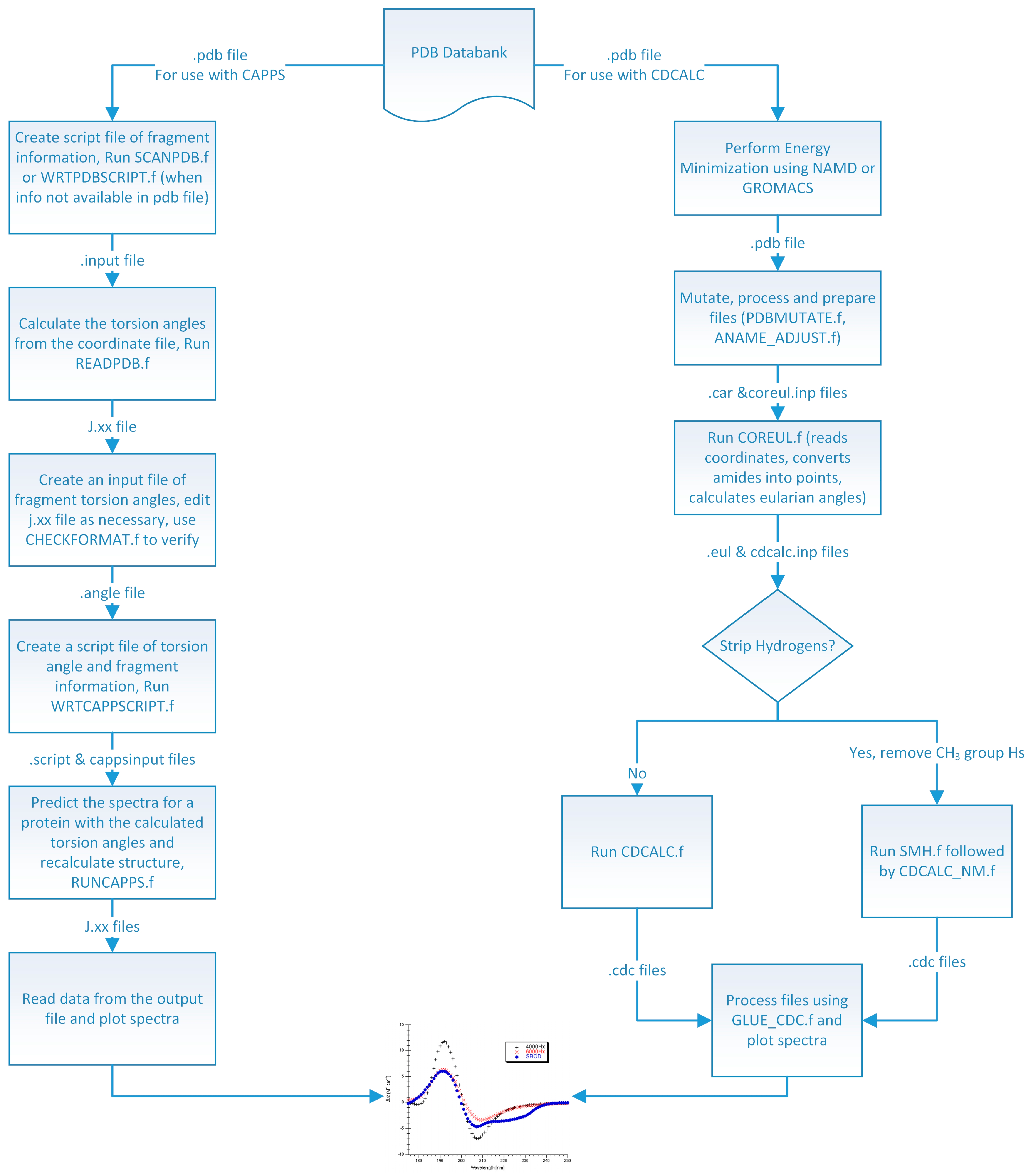
High quality structures were needed to predict circular dichroism for each protein so considerable effort was spent in preparing the model structures used (
Figure 8). In the DInaMo package the user has a choice to either use molecular mechanics to add hydrogens and minimize the structure or extract the internal coordinates and rebuild the protein’s secondary structural components (including hydrogens) using idealized bond lengths and angles. Currently, DInaMo treats only aliphatic amino acids (alanine, valine, proline, glycine, leucine, and isoleucine) in their entirety; all other amino acids are mutated. Typically, alanine is chosen because it can be initially approximated from the current side chain and will not introduce strain into the backbone. Alternatively, the protein structure can also be rebuilt to account for only the secondary structure fragments using the CAPPS route (
Figure 8). This automatically mutates any amino acid residues that are not currently treated to alanine before optimizing and reconstructing the structure. The molecular mechanics route (CDCALC,
Figure 8) requires significant energy minimization to adjust bond lengths, bond angles, and to average the positions of the hydrogen atoms that needed to be added; it is common for crystal structure geometries to have slightly short bond lengths (e.g., see Carlson
et al. 2005 as an example [
70]) so that they cannot be used directly with the dipole interaction model. Furthermore, the dipole interaction model is sensitive to small changes in structure [
9,
70,
71,
72]. Energy minimization is followed by mutation of the nonaliphatic residues and another brief minimization to relax any atomic clashes, when minimized with Insight
®II; these minimizations do not lead to changes in secondary structures, but impact highly flexible regions. It is the initial minimization that changes the flexible regions the most and not the post mutation minimization. When performed in NAMD, only one minimization was necessary.
Protein databank (PDB) [
73] files of the protein structures used (
Table 6) provide initial structures for the calculations. Hydrogen atoms were added to each protein structure as needed because they are required for the CD calculation. The particular PDB files were chosen for two reasons: (1) Each was a high-resolution structure with a R factor of less than 2.50 Å; (2) The structures chosen were the same species for which synchrotron radiation circular dichroism (SRCD) was available in the Protein Circular Dichroism Data Bank (PCDDB) [
44]. The only exception was crambin, for which only conventional CD was available [
63], but very high resolution crystal structures were available [
65]
Table 6.
PDB Structures and Literature CD Used.
Table 6.
PDB Structures and Literature CD Used.
| Protein Name | PDB Code | Resolution (Å) | CATH Fold [57] | PCDDB Code |
|---|
| Avidin | 2A8G [74] | 1.99 | mainly β | CD0000008000 [47] |
| Bacteriorhodopsin | 1QHJ [75] | 1.90 | mainly α | CD0000101000 [59] |
| Bovine pancreatic trypsin inhibitor | 5PTI [76] | 1.00 | irregular | CD0000007000 [47] |
| Calmodulin | 1LIN [77] | 2.00 | mainly α | CD0000013000 [47] |
| Crambin | 1AB1 [65] | 0.89 | α/β | Not applicable/[63] |
| Concanavalin A | 1NLS [78] | 0.94 | mainly β | CD0000020000 [47] |
| Cytochrome c | 1HRC [79] | 1.90 | mainly α | CD0000021000 [47] |
| Ferredoxin | 2FDN [80] | 0.94 | α/β | CD0000032000 [47] |
| Insulin | 3INC [81] | 1.85 | not classified | CD0000040000 [47] |
| Jacalin | 1KU8 [82] | 1.75 | mainly β | CD0000041000 [47] |
| Lectin (lentil) | 1LES [83] | 1.90 | mainly β | CD0000043000 [47] |
| Lectin (pea) | 1OFS [73] | 1.80 | mainly β | CD0000053000 [47] |
| Leptin | 1AX8 [84] | 2.40 | mainly α | CD0000044000 [47] |
| Light Harvesting Complex II | 1NKZ [67] | 2.00 | irregular/mainly α | CD0000114000 [59] |
| Lysozyme | 2VB1 [56] | 0.65 | mainly α | CD0000045000 [47] |
| Myoglobin (horse) | 3LR7 [85] 2V1K [86] | 1.25 | mainly α | CD0000047000 [47] |
| Myoglobin (sperm whale) | 2JHO [87] | 1.40 | mainly α | CD0000048000 [47] |
| Monellin | 1MOL [88] | 1.70 | α/β | CD0000046000 [47] |
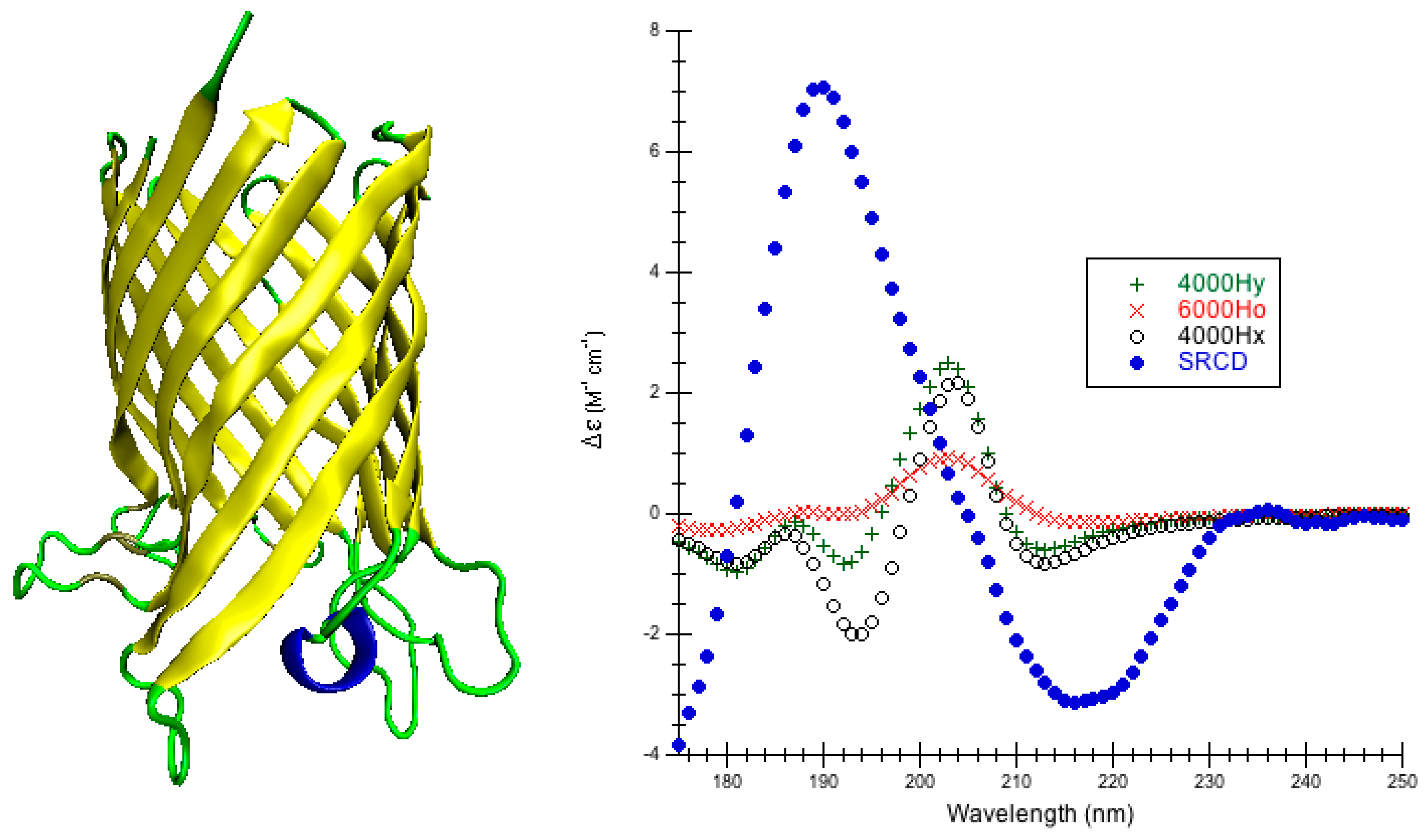
| Outer Membrane Protein G | 2IWV [62] | 2.30 | mainly β | CD0000118000 [59] |
| Outer Membrane Protein OPCA | 2VDF [61] | 1.95 | mainly β | CD0000119000 [59] |
| Phospholipase A2 | 1UNE [89] | 1.50 | mainly α | CD0000059000 [47] |
| Rhomboid peptidase | 2NR9 [58] | 2.20 | mainly α | CD0000109000 [59] |
| Rubredoxin | 1R0I [90] | 1.50 | mainlyβ | CD0000064000 [47] |
| Triose phosphate isomerase | 7TIM [64] | 1.90 | α/β | CD0000070000 [47] |
Figure 8.
Flow Diagram of the DInaMo Package. Note, the CD spectrum, like the one pictured at the bottom of this diagram, can only be displayed using a common graphing program such as Origin or Kaleidagraph.
Figure 8.
Flow Diagram of the DInaMo Package. Note, the CD spectrum, like the one pictured at the bottom of this diagram, can only be displayed using a common graphing program such as Origin or Kaleidagraph.
3.1. Energy Minimization (for use with CDCALC)
Each protein structure was minimized either with the Discover module of Insight
®II (San Diego, CA, USA) or with NAMD [
91]. Minimization was necessary to tweak the internal coordinates so that the structures could be used with the dipole interaction model. No major secondary structure elements were changed during the minimizations.
3.1.1. NAMD
Each protein was minimized in vacuum via the conjugate gradient method. The minimization was performed using the CHARMM22 [
92,
93] force field in NAMD [
91] for either 5000 or 10,000 steps. Larger proteins or lower resolution structures needed the larger number of steps for minimization. The structure at the last step of the minimization was used for CD predictions since no convergence criterion was required.
3.1.2. Insight®II/Discover
Using the force field CVFF (Consistent-Valence Force Field) [
94] within the Discover module of Insight
®II (San Diego, CA, USA) has proven highly successful with small peptide structures used with the dipole interaction model [
39,
70,
72] so that it was also applied to the proteins insulin, lysozyme, two species of myoglobin. Because solvent effects were not the object of this study, it was not deemed necessary to explicitly include the solvent in the Discover minimizations. A strategy of steepest descents followed by conjugate gradients was performed for the different proteins where the number of minimization steps varied for each protein. A large number of steps of steepest descents were chosen first to stay in a local minimum, followed by a short number of steps using conjugate gradients to just tweak the local minimum. For example, 900,000 steps of steepest descents and 100,000 steps of conjugate gradient were performed for lysozyme. The two myoglobins were minimized with 110,000 steps of steepest descents and 21,000 steps of conjugate gradients. Insulin only needed 1000 steps of steepest descents and 100 steps of conjugate gradients. These many iterations were needed to fine-tune the structure enough for use in circular dichroism (CD) calculations that included hydrogens. A final maximum derivative convergence criterion 0.001 was met for all minimizations upon completion of the conjugate gradients minimization.
3.2. CD Calculation
3.2.1. CDCALC
Cartesian coordinates generated within Insight
®II or NAMD were used to calculate the π-π* amide transitions of the protein using the dipole interaction model (DInaMo) [
31,
32,
35]. With this method, coordinates for the nonchromophoric atoms of the protein were treated directly, while the chromophoric amides were reduced to a single point located along the C-N bond of the amide. For the structures generated via NAMD, the hydrogens on CH
3 groups were deleted; the minimizations with Insight
®II included these hydrogens as isotropic polarizabilities. All secondary structure types including α-helices, β-sheets, turns, poly-
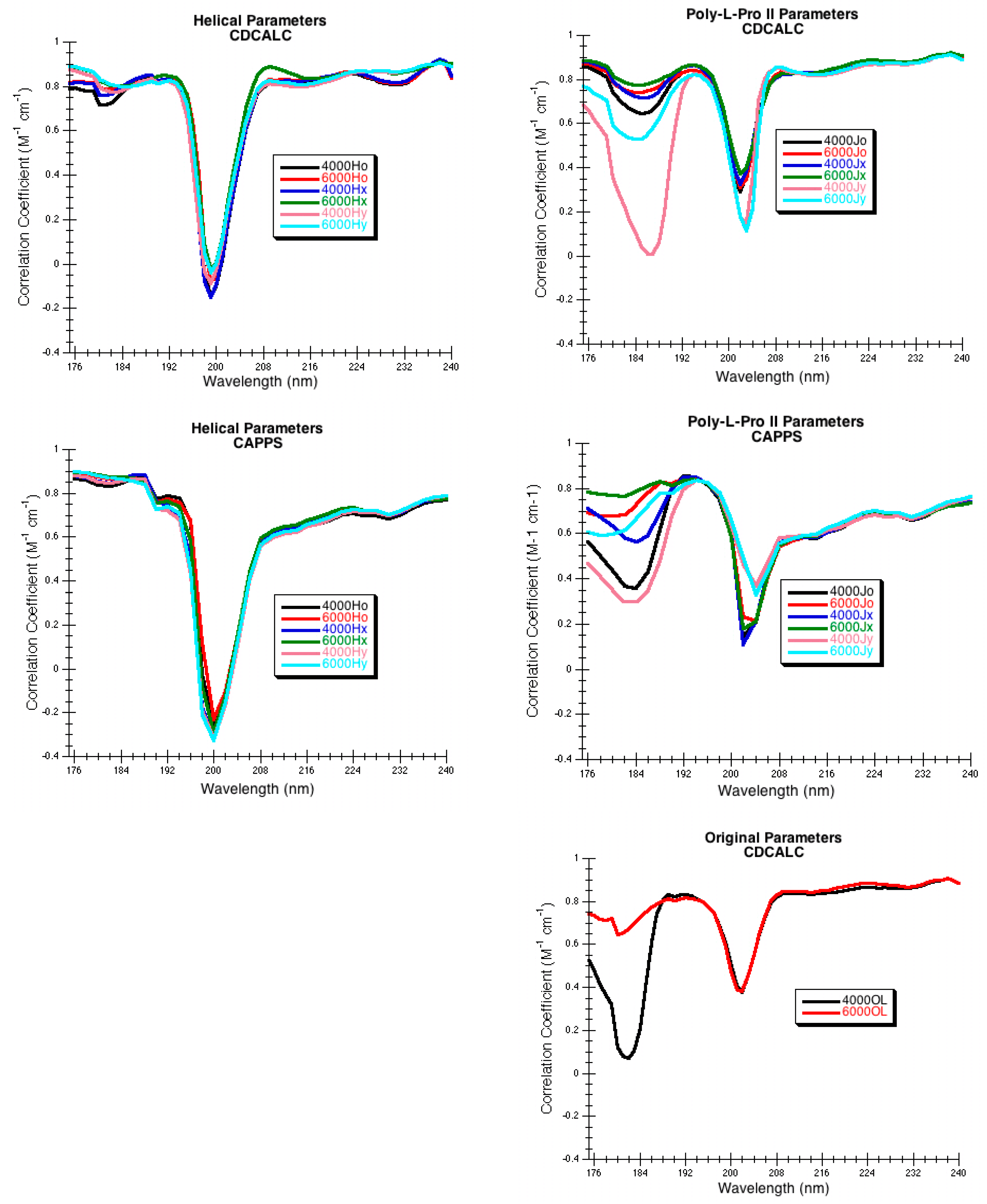
l-proline, and irregular structures are included in the calculation, so that no secondary structure is ignored. This is a major difference between CDCALC and CAPPS (see 3.3.2 CAPPS). The amide point position for the anisotropic chromophore was either the center of the N-C bond (o), shifted along the N–C bond 0.1 Å towards the carbonyl carbon (x), or shifted 0.1 Å normal to the C–N bond from the center into the NCO plane toward the carbonyl O (y). The Eulerian angles between the first amide chromophore and successive ones were calculated (COR_EUL in
Figure 8). The CDCALC portion of the program generated the normal modes and spectrum for each protein. Three different dispersive parameters were tested: the original parameters created for the dipole interaction model (OL) [
95], the α-helical parameters created for proteins (H) [
36], and the poly-
l-proline II parameters (J) [
36]. The CD spectrum using CDCALC of each protein was computed between 175 and 250 nm with a step size of 1 nm with bandwidths of either 4,000 or 6000 cm
−1. CDCALC for each protein was run on a Linux server (Fedora Core Linux 6, 64-bit) and was compiled using PGI FORTRAN 77 compiler.
3.2.2. CAPPS
CAPPS functioned by breaking the PDB structure into secondary structural elements of α-helices and β-sheets and rebuilding them using idealized bond lengths and bond angles; torsion angles were retained from the PDB structure. Other parts of the protein structure were ignored. For example, lysozyme had two partial turn structures that were ignored (
Table 7). For sperm whale myoglobin, one undefined secondary structure with residues 1–2 (VL), and one kink in a helix with residues 35–37 (GHP) were ignored (
Table 7). If more than 50% of the protein needed to be ignored because of close contacts occurring during the rebuild, then CAPPS was considered a failure for that protein. Like CDCALC, once CAPPS identified the secondary structures and rebuilt them, coordinates for the nonchromophoric atoms including all hydrogens were treated directly, while the chromophoric amides were reduced to a single point located along the C–N bond of the amide. The amide point position was either the center of the N–C bond (o), shifted 0.1 Å towards the carbonyl carbon (x), or shifted 0.1 Å normal to the C–N bond, toward the carbonyl O (y). The Eulerian angles between the first amide chromophore and successive ones were calculated, normal modes were generated, and the spectrum predicted. Only the helical (H) and poly-
l-proline II (J) parameters were tested as recommended by Bode and Applequist [
3]. The CD was computed between 176 and 250 nm with a step size of 2 nm with bandwidths of either 4000 or 6000 cm
−1. CAPPS for each protein was run on a Linux cluster that has 28 compute nodes, each of which has a dual 64-bit, 4-core Opteron processor and 16 GB of RAM.
3.3. CD Analysis
The results from the CD calculations were analyzed using Excel (Microsoft, Santa Rosa, CA, USA) and plotted with either Excel, OriginPro™ 7.5 (OriginLab Corporations, Northampton, MA, USA), or KaleidaGraph (Synergy Software, Reading, PA, USA). Published CD spectra were compared with the calculated values for each molecule. Further quantitative analysis was done by evaluating the normalized root mean square deviation (RMSD) between experiments and calculated at each wavelength for the total number of wavelengths
nλ computed.
4. Conclusions
Because the dipole interaction model is very sensitive to molecular geometry, it is crucial to optimize any protein structure either by energy minimization or rebuilding the secondary structure based on the torsions extracted from the PDB file. Current calculations suggest that energy minimization is an excellent choice for dealing with the geometric sensitivity and will less likely lead to failure than the rebuilding method, particularly if there are a significant number of β-sheets in the proteins.
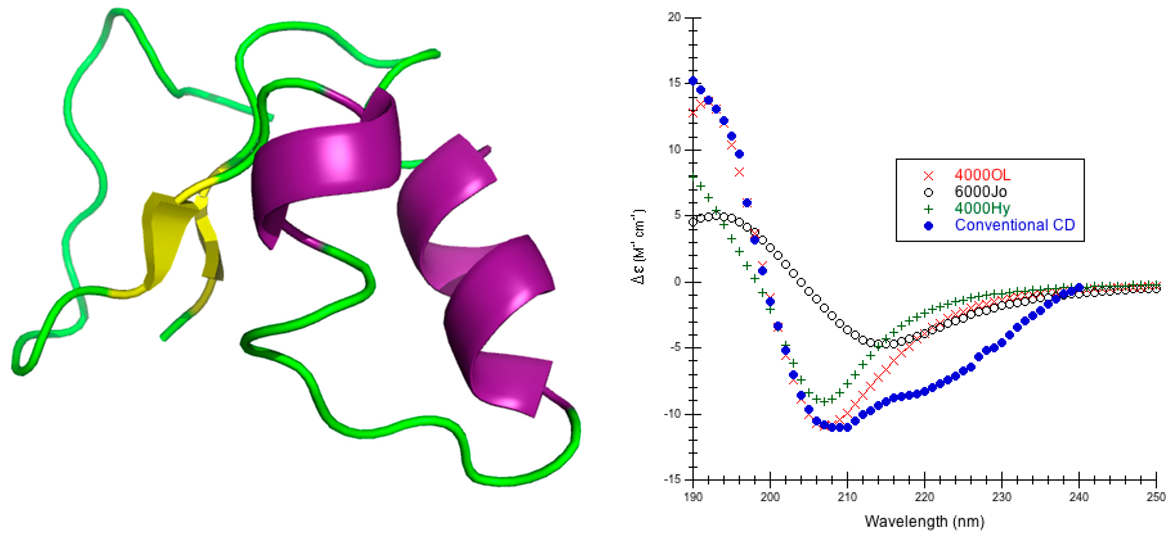
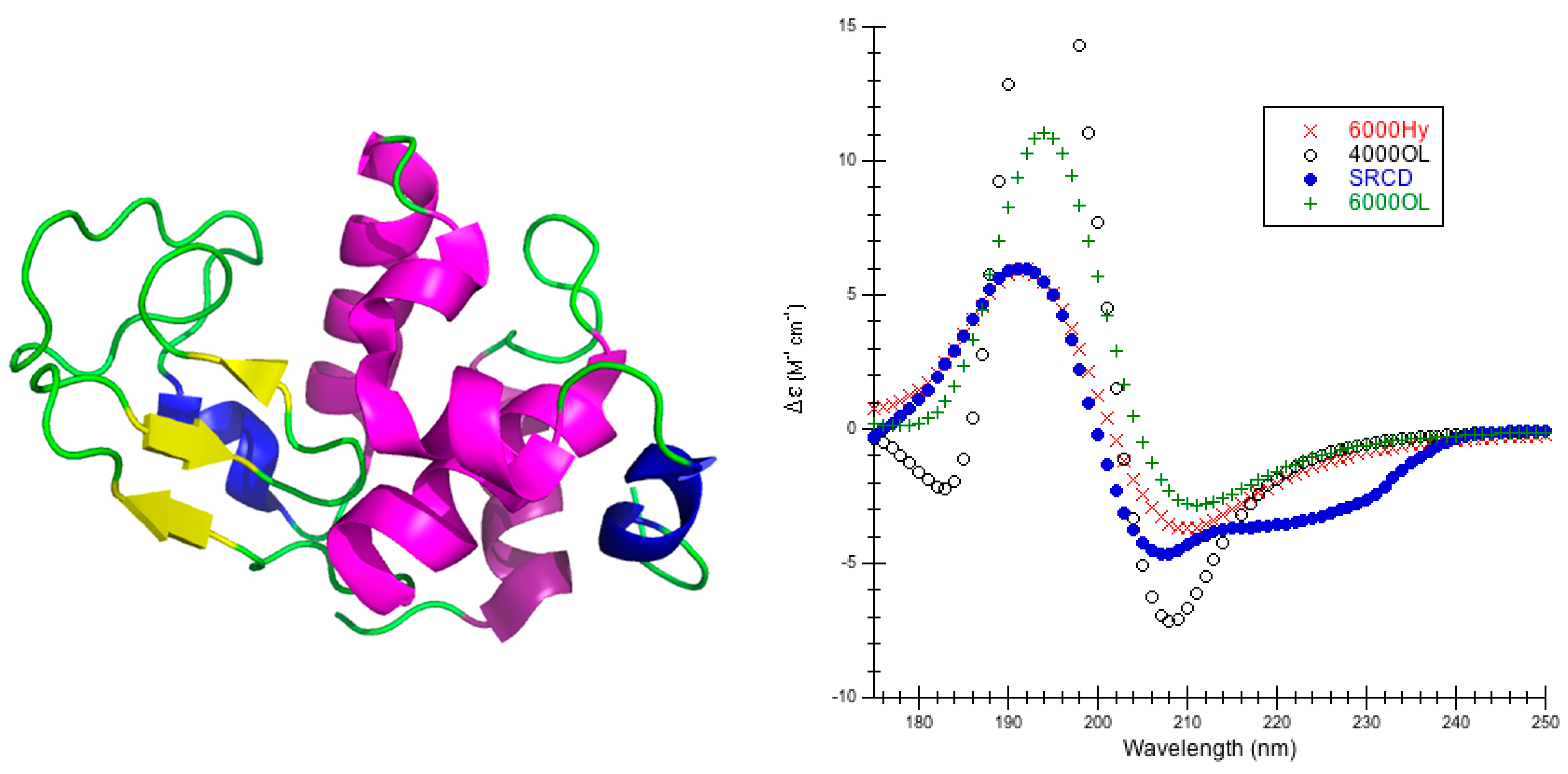
The choice of parameters for use with DInaMo depends on the fold and algorithm used. The best choice of parameters for mainly alpha proteins using CDCALC is 6000 OL and using CAPPS is 6000 Ho. The best choice of parameters for mainly beta proteins is the 4000 Hy with both CDCALC and CAPPS. Alpha/beta proteins are best treated with 4000 OL using CDCALC and 4000 Hx using CAPPS. Other kinds of structures, especially irregular ones, are best treated with 6000 Jy. For any unusual or new folds, the user should continue to test all parameters sets when performing CD calculations, and this includes testing different bandwidths. Bandwidths around 4000 to 6000 cm−1 are recommended for calculations to approximate the experiment far-UV CD spectrum of proteins.
DInaMo/CDCALC is an excellent choice for simulating the far-UV CD in the π-π* region. Using energy-minimized structures ignoring the hydrogens on CH
3 groups is the best current choice with DInaMo. More minimization is better than less, but 5000 conjugate gradient steps seems sufficient for small proteins with 150 amino acids or fewer, and 10,000 steps work better for 150–300 amino acids. For proteins larger than 300 amino acids, it is recommended to break the structure down into pieces 300 amino acids or fewer as long as no major secondary structures are disrupted [
96] and then use CDCALC, but be sure to minimize the intact protein first.
Because the removal of the hydrogens on CH3 groups is successful, removing more Hs (e.g., from CH2 or CH groups) is being explored. Furthermore, creating new isotropic polarizability parameters for CH3, CH2 and CH groups that treat the points as mean polarizabilities is also being explored. Plans to add and optimize parameters for the n-π* transition are also beginning.
The code for DInaMo is available upon request from the corresponding author, Kathryn. A. Thomasson at University of North Dakota, Chemistry Department, 151 Cornell St. Stop 9024, Grand Forks, ND 58202, USA.
Table 7.
PDB Structures Computed Using CAPPS and Fragments Ignored.
Table 7.
PDB Structures Computed Using CAPPS and Fragments Ignored.
| Protein Name | PDB Code | Fragments Ignored |
|---|
| Avidin | 2A8G [74] | Turn (54A-54A), Turn (60A-62A), Turn (112A-112A) |
| Bacteriorhodopsin | 1QHJ [75] | Turn (5A-5A), Turn (33A-36A), Turn (101A-104A), Turn (128A-130A), Turn (161A-164A) |
| Bovine pancreatic trypsin inhibitor | 5PTI [76] | Turn (1A-1A), Turn (46A-46A), Turn (57A-58A), Sheet (45A-45A) |
| Calmodulin | 1LIN [77] | Turn (3A-5A), Turn (27A-28A), Turn (100A-101A), Turn (146A-148A) |
| Crambin | 1AB1 [65] | Turn (1A-2A), Sheet (32A-34A) |
| Cytochrome c | 1HRC [79] | Turn (1A-1A), Turn (15A-48A), Turn (69A-69A), Helix (2A-14A) |
| Concanavalin A | 1NLS [78] | Coil (1A-3A), Coil (11A-13A), Coil (79A), Coil (150A-152A), Coil (153A-155A) |
| Ferredoxin | 2FDN [80] | CAPPS FAILED |
| Insulin | 3INC [81] | C-terminus (21A), N-terminus (1B-7B), Turn (21B-23B), Helix (18A-20A), Sheet (24B-26B) |
| Jacalin | 1KU8 [82] | CAPPS FAILED |
| Lentil Lectin | 1LES [83] | Turn (1A-1A), Helix (98A-100A), Turn (62A-69A), Turn (180A-182A), Turn (190A-192A) |
| Pea Lectin | 1OFS [73] | CAPPS FAILED |
| Leptin | 1AX8 [84] | Turn (3A-3A), Turn (24A-50A), Turn (residues 68A-70A), Turn (144A-146A) |
| Light Harvesting Complex II | 1NKZ [67] | Turn (2A-4A), Turn (10A-10A) |
| Lysozyme | 2VB1 [56] | Turn (1A-3A), Turn (116A-118A), Sheet (43A-45A), Sheet (51A-53A) |
| Myoglobin (horse) | 3LR7 [85] 2V1K [86] | Turn (1A-2A), Turn (21A-19A), Turn (59A-57A), Turn (97A-99A), Turn (151A-153A) |
| Myoglobin (sperm whale) | 2JHO [87] | Turn (1A-2A), Turn (19A-19A), Turn (37A-35A), Turn (97A-99A) |
| Monellin | 1MOL [88] | CAPPS FAILED |
| Outer Membrane Protein G | 2IWV [62] | CAPPS FAILED |
| Outer Membrane Protein OPCA | 2VDF [61] | CAPPS FAILED |
| Phospholipase A2 | 1UNE [89] | Turn (1A-1A), Turn (58A-58A), Helix (18A-21A), Helix (113A-115A) |
| Rhomboid peptidase | 2NR9 [58] | Turn (29A-29A), Turn (40A-42A), Turn (86A-84A), Turn (193A-195A) |
| Rubredoxin | 1R0I [90] | Turn (1A-3A), Turn (48A-48A), Sheet (4A-6A), Helix (45A-47A) |
| Triose phosphate isomerase | 7TIM [64] | Turn (2A-4A), Turn (87A-89A), Turn (119A-121A), Turn (128A-130A), Turn (136A-138A), Turn (237A-237A) |


