1. Introduction
Multi-component membranes consisting of a small number of lipids provide simple model systems for biological membranes, which contain a huge number of different lipid and protein components. Since membranes are essentially 2-dimensional systems, they can attain different thermodynamic phases and undergo phase transitions between these phases. From a biological perspective, the most interesting phase transitions are provided by transitions between two distinct
liquid phases, in which the membrane molecules can undergo fast lateral diffusion within all membrane domains [
1]. The corresponding two-phase coexistence regions lead to critical points that belong to the universality class of the 2-dimensional Ising model [
2].
The simplest examples for fluid-fluid coexistence in membranes are presumably found in binary mixtures of cholesterol and a single phospholipid. Indeed, a variety of spectroscopic methods such as deuterium nuclear magnetic resonance [
3–
5] were applied to such binary mixtures and provided evidence for the formation of intramembrane domains. The underlying mechanism for this domain formation has been a matter of some debate as reviewed in [
6]. In this theoretical study, we will not address this controversy but take the fluid-fluid coexistence of cholesterol/phospholipid mixtures proposed in [
4,
5,
7] and recently reviewed in [
8] as a motivation to study a generic model for this kind of two-phase coexistence.
For ternary mixtures consisting of an unsaturated phospholipid, sphingomyelin, and cholesterol, as originally studied in the context of sphingolipid-cholesterol rafts [
9], the formation of liquid-ordered and liquid-disordered domains can be directly observed by fluorescence microscopy. In this way, phase separation in ternary mixtures has been studied for a variety of membrane systems including giant vesicles [
10–
15], solid-supported membranes [
16–
18], hole-spanning (or black lipid) membranes [
19], as well as pore-spanning membranes [
20]. The phase diagrams of such three-component membranes have been determined using spectroscopic methods [
5] as well as by fluorescence microscopy of giant vesicles and X-ray diffraction of membrane stacks [
21–
24]. Furthermore, fluid-fluid coexistence has also been found in giant plasma membrane vesicles that contain a wide assortment of lipids and proteins [
25,
26].
In this paper, we consider the effect of adhesion onto the phase behavior of multi-component membranes. We first emphasize that many adhesion geometries lead to a segmentation of the membranes. Examples are provided by the adhesion of vesicles, by hole- or pore-spanning membranes, and by membranes supported by chemically patterned surfaces. In all of these cases, the adhesion leads to two distinct membrane segments that experience different environments. These environments attract the different molecular components of the membrane with different affinities, i.e., each environment acts to recruit certain components and to expel others. As a consequence, the compositions of the two membrane segments are different as well.
We will focus on the simplest example for fluid-fluid coexistence as provided by two-component membranes and study the adhesion effects by generalizing a generic lattice model for binary mixtures. This lattice model corresponds to a semi-grand canonical description and depends on the relative chemical potential for the two molecular species. Using this model, it is relatively easy to see that the adhesion-induced segmentation of the membranes leads, in general, to two distinct phase transitions in the two membrane segments. In order to obtain theoretical predictions that are accessible to experiments, we then consider the mole fractions in the two membrane segments and show how one can obtain the phase behavior in terms of these mole fractions. One important parameter turns out to be the affinity contrast, which describes the different molecular interactions between the two membrane segments and their environments.
We show that the fluid-fluid coexistence region as found for the two-component membrane in a uniform environment is replaced, for any nonvanishing affinity contrast, by two distinct coexistence regions, which are separated by an intermediate one-phase region. The relative sizes and positions of these different regions are shown to depend only on a relatively small number of parameters, namely temperature, mole fraction of one molecular species, area fraction of one of the membrane segments, and affinity contrast. For the generic case of a nonzero affinity contrast, our theory predicts that phase separation can only occur separately in each of the two membrane segments but not in both segments simultaneously. Furthermore, adhesion is also found to suppress the phase separation process within certain regions of the phase diagrams.
Our paper is organized as follows. First, Section 2 contains a brief review of fluid-fluid coexistence in two-component membranes and Section 3 describes the lattice binary mixture as a generic model for phase separation in two dimensions. In Section 4, we discuss several adhesion geometries such as vesicle adhesion and pore-spanning membranes, and describe how these geometries lead to a segmentation of the membranes into two different membrane segments. These segments experience distinct environments, which can be characterized by relative affinities. In Section 5, we introduce the lattice model for the adhering membranes and show that the relative affinities of the two membrane segments lead to shifts of the relative chemical potential. It is then relatively easy to conclude that the adhering membranes undergo two phase transitions. In order to obtain theoretical predictions that are accessible to experiments, we then replace in Section 6 the relative chemical potential by the mole fraction Xa of the a-molecules and explain how one can obtain the phase diagrams as a function of Xa and temperature. The results for these phase diagrams are then described in Section 7. At the end, we give a brief summary and outlook.
2. Liquid-Liquid Coexistence in Two-Component Membranes
At constant pressure, the phase diagrams of multi-component membranes depend on the ambient temperature T and on the composition of the membranes. For membranes consisting of two molecular species, say a and b, and containing Naa-molecules and Nbb-molecules, the composition is described by the mole fractions
one of which can be varied independently.
Thus, phase diagrams of two-component membranes are conveniently described in the (
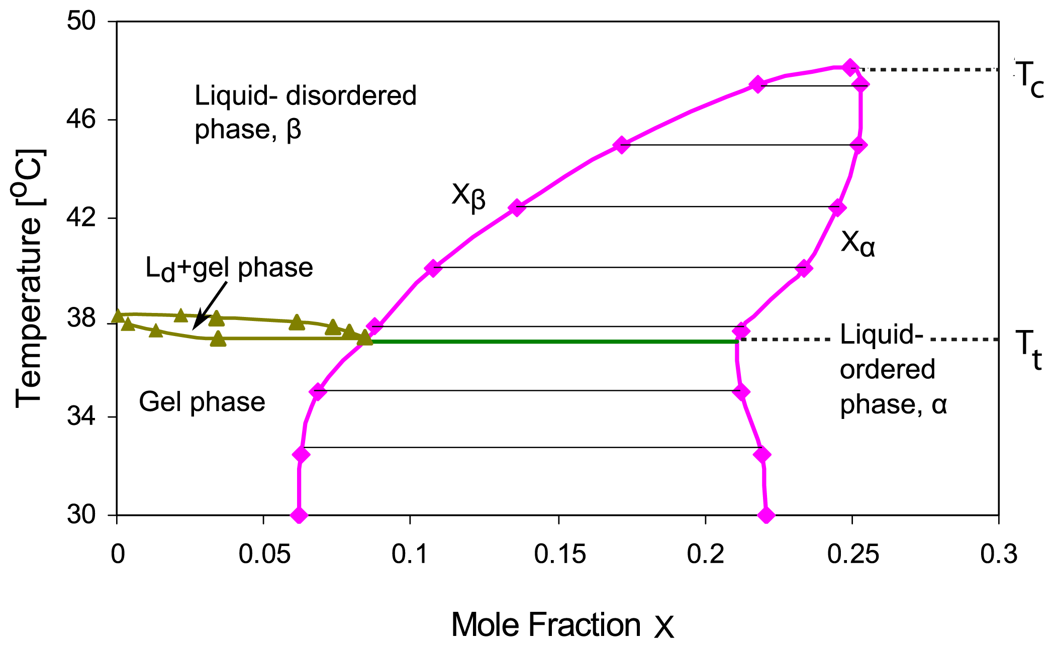
Xa, T)-plane. For binary mixtures of phospholipid and cholesterol, the phase diagrams deduced from deuterium nuclear magnetic resonance spectroscopy exhibit a coexistence region for the liquid-ordered phase, say
α, which is rich in cholesterol, and the liquid-disordered phase, say
β, which is poor in cholesterol [
3–
5,
7,
8], see
Figure 1.
The membrane undergoes phase separation into the α and β phases within the temperature range Tt< T < Tc, i.e., above the triple point temperature T = Tt and below the critical temperature T = Tc. The αβ coexistence region can then be described by
with the two binodal lines
3. Lattice Model for Two-Component Membranes
A relatively simple but instructive model for two-component membranes is provided by lattice binary mixtures, in which the configurations of the two molecular components are described by occupation numbers [
27–
31]. The two-dimensional lattice binary mixture is equivalent to the two-dimensional Ising model. Therefore, both exact results from the Ising model as well as approximation schemes such as the mean field approximation can be used to determine the phase diagrams of this lattice model.
3.1. Lattice Description of Large Membrane Segments
To proceed, let us first consider a large membrane segment with total area
, which is disretized into a square lattice Ω with lattice sites i and lattice constant
. The total number of lattice sites will be denoted by
Since the discretization lattice is characterized by a single lattice constant
, both the a- and the b-molecules are described here by the same molecular area A.
Within the framework of the lattice binary mixture, the molecular configurations of the two-component membrane are now described in terms of occupation numbers
The mole fraction Xa of the a-molecules is now given by the expectation value of the occupation number ni, i.e.,
The total number Na of a-molecules is given by Na = ∑ini and the total number Nb of b-molecules by
Thus, for the lattice binary mixture, the total number of a- and b-molecules is fixed and given by Na + Nb = |Ω|. This constraint on the two molecular numbers implies that the lattice binary mixture describes a semi-grand canonical ensemble, see further below.
3.2. Configurational Energy of Binary Mixture
If two neighboring sites i and j of the lattice are both occupied by a molecules, these molecules have the interaction energy Uaa. Likewise, two neighboring b molecules interact via the interaction energy Ubb and two neighboring sites occupied by one a- and one b-molecule contribute the interaction energy Uab. For the unbound membrane segment, the configuration-dependent interaction energy is then given by
and the total configurational energy {n} has the form
where we have introduced two chemical potentials
μa and
μb for the
a- and
b-molecules. Since the molecular numbers
Na and
Nb satisfy the constraint (
7), this configurational energy is equivalent to
with the relative chemical potential
The term
μb|Ω| on the right hand side of (
10) can be omitted because it does not depend on the occupation numbers {
n} and, thus, cancels out from all expectation values calculated with the statistical weight exp(−
{
n}
/kBT).
The form (
10) of the configurational energy shows explicitly that the lattice binary mixture represents a semi-grand canonical ensemble [
32,
33], which depends on the total number |Ω|
A of membrane molecules and on the relative chemical potential Δ
μ. This ensemble is appropriate here because membranes have a fixed surface area and we use the simplifying assumption that both molecular species have the same molecular area. Therefore, when the system exchanges
a- and
b-molecules with the corresponding chemical reservoirs, we have to remove
b-molecules when we want to insert
a-molecules and
vice versa.
3.3. Phase Behavior of Binary Mixture
The lattice binary mixture just described is equivalent to the two-dimensional Ising model if one expresses the molecular configurations {n} in terms of the spin variables σi ≡ 2ni − 1. This equivalent Ising model depends only on two parameters, the dimensionless temperature
and the dimensionless ordering field
The Ising system undergoes phase separation for
H̄ = 0 and 0 ≤
T̄ < T̄c, where
T̄c denotes the critical temperature. The exact value of the critical temperature is given by [
34]
for the Ising model on a square lattice. As we approach the line
H̄ = 0 from positive and negative values of
H̄, the order paramter 〈
σi〉 attains the values 〈
σi〉 = + ϒ (
T̄) and 〈
σi〉 = −ϒ (
T̄), respectively, with the spontaneous order parameter [
34]
The corresponding phase transition in the lattice binary mixture occurs at the relative chemical potential
As we approach the transition value Δμ = μαβ of the relative chemical potential from below or from above, the mole fraction Xa = 〈ni〉 approaches the values
respectively, with the function ϒ (
T̄) as given by (
15). These two mole fractions define the binodal lines
Xa =
Xa,β(
T̄) and
Xa =
Xa,α in the (
Xa, T̄) phase diagram of the lattice binary mixture. This phase diagram is symmetric with respect to the transformation
, which reflects the particle-hole symmetry of the lattice binary mixture.
3.4. Relative Chemical Potential as a Function of Mole Fraction
The semi-grand canonical ensemble of the lattice binary mixture is not particularly convenient from an experimental point of view since the relative chemical potential Δμ does not represent an experimental control parameter. Instead of Δμ, one typically controls the mole fraction Xa. If we consider Xa as an independent thermodynamic variable, the relative chemical potential becomes a dependent variable that will be described by the functional relationship
The change from Δμ to Xa corresponds to a Legendre transformation from the semi-grand canonical ensemble to the canonical ensemble. Even though the form of the function G is not known explicitly (because we have no exact solution for the 2-dimensional Ising model in a finite ordering field, H̄ ≠= 0), thermodynamics implies some useful properties of G(Xa).
First, it follows from thermodynamic stability that the chemical potential
μa of the
a-molecules must be a non-decreasing function of
Xa, see, e.g., [
35]. Likewise, the chemical potential
μb of the
b-molecules must be a non-decreasing function of
Xb = 1 −
Xa, which implies that it must be a non-increasing function of
Xa. It then follows that the relative chemical potential Δ
μ =
μa −
μb as a function of
Xa must satisfy
More precisely, the function Δμ = G(Xa) has a strictly positive derivative,
and stays constant with
It then follows that
G(
X) is a monotonically increasing function of
X for 0
< X < Xa,β(
T̄), stays constant for
Xa,β(
T̄) ≤
X ≤
Xa,β(
T̄), and continues to increase monotonically for
Xa,β(
T̄)
< X < 1, where the two binodals are explicitly given by (
17).
5. Lattice Model for Adhering Membranes
We will now extend the lattice binary mixture as described in Section 3 to adhering membranes with two membrane segments as in
Figures 2 and
3. We are then led to consider two sublattices that experience different interactions as described by the relative affinities of the two membrane segments.
5.1. Two Sublattices for Two Membrane Segments
Consider an adhering membrane partitioned into two segments,
and
. The discretization of such a membrane leads to two sublattices, Ω[1] and Ω[2]. Sublattice Ω[1] for segment
consists of
lattice sites whereas sublattice Ω[2] for segment
has
such sites. As before, the symbol A denotes the area per lattice site and corresponds to the molecular area of the a- and b-molecules. The area fraction q[1] of segment
is now equal to
5.2. Configurational Energy of Adhering Membranes
The configurations of a- and b-molecules within an adhering membrane are again described in terms of the occupation numbers {ni}, where ni = 1 represents an a-molecule as before. The configurational energy of this membrane now contains additional terms arising from the interaction potentials Ua[m] and Ub[m] for the a- and b-molecules with the corresponding environments. More precisely, membrane segment
contributes the additional energy term
with the relative affinity Δ
U[m] as in (
33) where the last
n-independent term on the right hand side can again be omitted because it does not affect the statistical properties of the system. Adding the
U-dependent energy term
U[m] in (
38) to the standard form (
10) for the configurational energy of the lattice binary mixture, the configurational energy of segment
becomes
where the interaction energy int[m] describes the molecular interactions between the a- and b-molecules within segment
. This interaction energy now has the form
which is identical with the expression (
8) apart from the summation that now includes only nearest neighbors 〈
ij〉 within the sublattice Ω
[m] corresponding to segment
.
The configurational energy of an adhering membrane consisting of two membrane segments is then given by
where the additional energy term
db{
n} arises from the domain boundaries between the two membrane segments. The latter term can be ignored compared to the first two terms in (
41) when we consider the limit of large membrane segments. Indeed, in this limit, the free energies obtained from the first two terms
[1]{
n} and
[2]{
n} increase as the segment areas
and
whereas the free energy arising from the domain boundary term
db{
n} increases only as the length of the domain boundary, which is of the order of
.
Therefore, in this large membrane limit, we are left with two membrane segments,
and
, each of which is governed by a configurational energy of the form (
39). In the semi-grand canonical ensemble of the lattice binary mixture, these large segments are only coupled via the relative chemical potential Δ
μ,
i.e., via the particle reservoirs for
a- and
b-molecules.
5.3. Phase Transitions in Membrane Segments
The configurational energy (
10) for the standard lattice binary mixture leads to a phase transition at the relative chemical potential Δ
μ =
μαβ = 2(
Uaa −
Ubb) for 0 ≤
T̄ < T̄c as described by (
16). Comparison of the configurational energy (
39) for the membrane segment
with the configurational energy (
10) for the standard model then shows that this segment undergoes a phase transition at the relative chemical potential
As long as the relative affinities ΔU[m] of the two membrane segments are different, i.e., as long as ΔU[2] ≠= ΔU[1], the two critical values μαβ[2] and μαβ[1] are different as well and the two segments undergo two distinct phase transitions. Therefore, the adhesion-induced partitioning into two membrane segments leads to two distinct phase transitions for ΔU[2] ≠= ΔU[1].
6. Phase Behavior in Terms of Mole Fractions
In order to make theoretical predictions that are accessible to experiment, we will now describe the phase behavior of the two membrane segments in terms of their mole fractions. Since the two membrane segments experience different environments and, thus, different relative affinities, they will, in general, differ in their compositions. Therefore, we have to distinguish the mole fraction Xa[1] in segment
from the mole fraction Xa[2] in segment
. To determine the two mole fractions Xa[1] and Xa[2], we need two independent relations between these two variables. As shown in the following section, one relation is obtained from the partitioning of the total number of a- and b-molecules between the two membrane segments, the other from the chemical equilibrium between these segments.
6.1. Partitioning of Membrane Molecules
One relation between the two mole fractions Xa[1] and Xa[2] is provided by the partitioning of the molecules between the two membrane segments. Because the total number |Ω| = |Ω[1]| + |Ω[2]| of molecules is fixed within the adhering membrane, the mole fractions Xa[1] and Xa[2] satisfy the relation
where
Xa is the overall mole fraction of the
a-molecules as before. Using the expression (
37) for the area fraction
q[1] and
q[2] = 1 −
q[1], the relation (
43) becomes
Note that this partitioning relation depends only on two parameters, the area fraction q[1] of segment
and the overall mole fraction Xa.
6.2. Relative Chemical Potentials of Membrane Segments
Comparison of the configurational energy (
39) of membrane segment
with the configurational energy (
10) of the standard lattice binary mixture shows that the relative chemical potential Δ
μ of the standard model is replaced byΔ
μ−Δ
U[m] for segment
. It then follows from (
19) thatΔ
μ−Δ
U[m] =
G(
Xa[m]),
i.e., membrane segment
is governed by the relative chemical potential
As explained in Section 3.4, thermodynamic stability implies that the function G(Xa[m]) is monotonically increasing for 0 < Xa[m]< Xa,β(T̄), attains the constant value
and continues to increase monotonically for
Xa,α(
T̄)
< Xa[m]< 1, where the two binodals
Xa,β(
T̄) and
Xa,α(
T̄) are explicitly given by (
17).
6.3. Chemical Equilibrium Between Membrane Segments and Affinity Contrast
Since the two membrane segments can exchange a- and b-molecules by lateral diffusion, they will reach a state of chemical equilibrium with
or
where we introduced the affinity contrast
between the two membrane segments with Δ
U1,2 = −Δ
U2,1. Thus, chemical equilibrium as described by (
48) provides a second relation between the two mole fractions
Xa[1] and
Xa[2]. This relation becomes particularly useful if one of the two segments undergoes phase separation because we can then replace one of the
G-terms by the constant value
μαβ. Furthermore, it is convenient to define the shifted function
which attains the value
and increases monotonically with
X outside of this interval. In terms of the shifted function Δ
G, the chemical equilibrium relation (
48) becomes
It is not difficult to see that any two mole fractions
Xa[1] and
Xa[2] that satify this equation and, thus, represent a solution of it do not depend on the shift
μαβ but only on the affinity contrast Δ
U2,1. Indeed, we can add any constant to the functions Δ
G(
X) or
G(
X) without changing the solution to (
52) or (
48).
6.4. Phase Separation in Segment
If segment
undergoes phase separation, the mole fraction Xa[1] must have a value within the range
and Δ
G(
Xa[1]) = 0 as in (
51). The chemical equilibrium relation (
52) then simplifies and becomes
We now have to distinguish two cases corresponding to zero and nonzero affinity contrast Δ
U2,1. If Δ
U2,1 = 0, the molecules experience the same relative affinities in both membrane segments and thus have no preference for either segment. We then conclude that the whole membrane undergoes phase separation and that
Xa[2] =
Xa[1] =
Xa, where the second equality follows from the partitioning relation (
44).
On the other hand, if Δ
U2,1 ≠ 0, the chemical equilibrium relation (
54) implies that Δ
G(
Xa[2]) ≠ 0,
i.e., that segment
does not undergo phase separation but represents a
spectator phase with uniform composition. The corresponding mole fraction
Xa[2] =
Xa,*[2] satisfies the implicit equation
and stays constant as long as the mole fraction
Xa[1] lies within the coexistence region (
53) of segment
. Note the subscript * that is used, here and below, to indicate the mole fractions of a spectator phase.
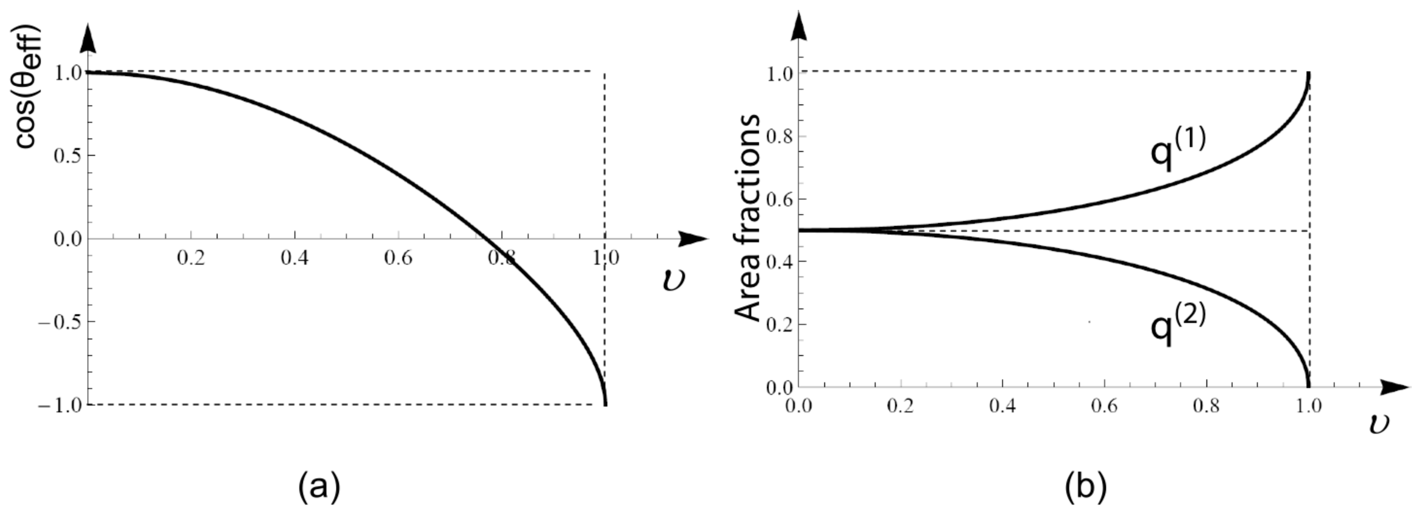
Because Δ
G(
x) increases monotonically with
x both for 0
< x < Xβ and for
Xα< x < 1, the implicit
equation (55) implies that the mole fraction
Xa,*[2] of the uniform spectator phase in segment
decreases monotonically with increasing affinity contrast Δ
U2,1 and satisfies
as well as
Furthermore, this mole fraction exhibits the limiting behavior
as well as
Therefore, as one increases the affinity contrast ΔU2,1 from large negative to small negative values, the mole fraction Xa,*[2] of the spectator phase in segment
decreases monotonically as a function of ΔU2,1, from Xa,*[2] = 1 to Xa,α(T̄) corresponding to the upper binodal. At ΔU2,1 = 0, this mole fraction jumps from the value Xa,α(T̄) for the upper binodal to the value Xa,β(T̄) for the lower binodal. Finally, as one increases the affinity contrast ΔU2,1 from small positive to large positive values, the mole fraction Xa,*[2] decreases monotonically from the value Xa,β(T̄) to Xa,*[2] = 0.
6.5. Phase Separation in Segment
Now, consider the situation, in which segment
of the adhering membrane undergoes phase separation. Repeating the arguments of the previous subsection, it then follows that the mole fraction Xa,*[2] of segment
satisfies
and that Δ
G(
Xa[2]) = 0 as in (
51). The mole fraction
Xa[1] in segment
then satisfies the implicit equation
which implies
where Xa,*[1] denotes the mole fraction of the uniform spectator phase in segment
.
Using again the general properties of the function Δ
G(
x), we find from (
61) that the mole fraction
Xa[1] =
Xa,*[1]increases monotonically with increasing affinity contrast
U2,1. More precisely, as one increases Δ
U2,1 from large to small negative values, the mole fraction
Xa,*[1] increases from
Xa,*[1] = 0 to
Xa,β(
T̄), jumps at Δ
U2,1 = 0 from
Xa,β(
T̄) to
Xa,α(
T̄), and finally increases monotonically from
Xa,α(
T̄) to
Xa,*[1] = 1 as the affinity contrast Δ
U2,1 is increased from small to large positive values. Thus, the mole fraction
Xa,*[1] satisfies
and
Furthermore, this mole fraction exhibits the limiting behavior
as well as
7. Phase Diagrams for Adhering Membranes
From an experimental point of view, it is most useful to describe the phase behavior in terms of overall composition and temperature. The corresponding phase diagrams can be derived by combining the partitioning relation (
44) with the chemical equilibrium relations as discussed in the previous subsections. Thus, inserting (i) the inequalities (
53) for the mole fraction
Xa[1] and (ii) the equalities (
56)–(
59) for the mole fraction
Xa[2] =
Xa,*[2] of the uniform spectator phase into the partitioning relation (
44), we obtain the binodals for the two-phase coexistence region of segment
in the (
Xa, T̄)-plane. Likewise, the binodals for the coexistence region of segment
in the (
Xa, T̄)-plane is obtained by inserting the inequalities (
60) for the mole fraction
Xa[2] and the equalities (
63)–(
66) for the spectator phase mole fraction
Xa[1] =
Xa[1],* into the partitioning relation (
44).
The two coexistence regions for the two membrane segments are separated by an intermediate one-phase region as long as the affinity contrast ΔU2,1 does not vanish, i.e., as long as the two membrane segments are characterized by different relative affinities ΔU[m] = Ua[m] − Ub[m]. Thus, for ΔU2,1 ≠ 0 or relative affinities ΔU[2] ≠ ΔU[1], the adhesion-induced partitioning into two segments leads to two distinct two-phase coexistence regions within the (Xa, T̄)-plane.
7.1. Parameter Dependence of Phase Diagrams
The phase diagrams of the adhering membranes in the (
Xa, T̄)-plane depend on the parameters that enter the partitioning relation (
44) and the chemical equilibrium relations. The partitioning relation (
44) contains only one parameter, the area fraction
q[1] of segment
, in addition to the overall mole fraction
Xa of the
a-molecules. The chemical equilibrium relations, on the other hand, involves the function Δ
G(
X) and the affinity contrast Δ
U2,1. The function Δ
G(
X) depends on the interaction parameters
Uaa, Uab, and
Ubb in the configurational energy (
40) via the dimensionless temperature
T̄ ≡ 4
kBT=(2
Uab −
Uaa −
Ubb) as introduced in (
12).
Therefore, for the lattice model considered here, the phase diagrams of the adhering membranes depend only on four parameters: (i) overall mole fraction Xa, (ii) dimensionless temperature T̄, (iii) area fraction q[1], a purely geometric parameter, and (iv) affinity contrat ΔU2,1.
The four-dimensional parameter space is most easily explored via two-dimensional slices. In the following, we will display two-dimensional phase diagrams that depend on the overall mole fraction
Xa and on the rescaled temperature
T̄ = T̄c =
T/Tc for fixed values of the area fraction
q[1] and of the affinity contrast Δ
U2,1, see
Figures 4–
7 below. This choice is convenient because it allows a direct comparison with the phase diagram of the two-component membrane in a uniform environment. The latter phase diagram, which depends only on mole fraction
Xa and on temperature, is recovered for the limiting values
q[1] = 0 and
q[1] = 1 of the area fraction as well as for vanishing affinity contrast Δ
U2,1 = 0. In the following, we will use the term “uni-env membrane” as an abbreviation for “membrane in a uniform environment”.
The phase diagrams in
Figures 4–
6 below are based on the exact binodals of the lattice binary model as described by (
17) and on the exact values of the spectator phase mole fractions
Xa,*[1] and
Xa,*[2] as given by (
63)–(
66) and (
56)–(
59) for small and large values of the affinity contrast. Therefore, the phase diagrams in
Figures 4–
6 are exact as well. In contrast, the phase diagrams in
Figure 7 are based on the mean-field approximation.
In all phase diagrams displayed in
Figures 4–
7 below, the two coexistence regions for the membrane segments are distinguished by their color: the coexistence regions of segment
are blue whereas the coexistence regions of segment
are red. Furthermore, the remaining white regions in the phase diagrams represent one-phase regions, in which the membranes attain uniform compositions without domains.
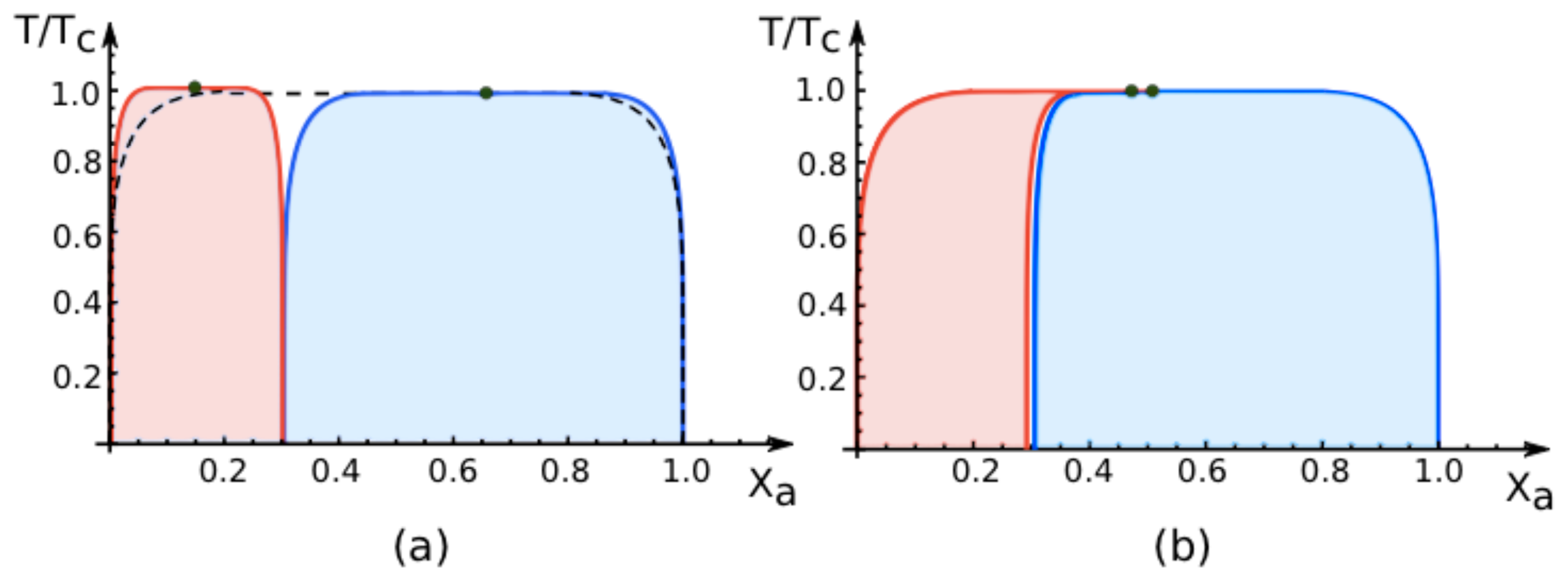
7.2. Phase Diagrams for Positive Affinity Contrasts
In
Figure 4, we display the phase diagrams of adhering membranes in the (
Xa, T/Tc)-plane as obtained from the lattice binary mixture for small and large
positive values of the affinity contrast Δ
U2,1 = Δ
U[2] − Δ
U[1] keeping the area fraction
q[1] of segment
constant. The relative affinities Δ
U[m] are related to the molecular interaction potentials
Ua[m] and
Ub[m] via Δ
U[m] =
Ua[m] −
Ub[m] which implies that
Because we use the sign convention that attractive interaction potentials are negative, see (
32), the second inequality in (
67) applies to systems, in which the
b-molecules prefer to stay in segment
while the
a-molecules prefer to stay in segment
. Therefore, as one increases the mole fraction
Xa starting from
Xa = 0, the
a-molecules are first enriched in segment
, which then undergoes phase separation leading to the blue coexistence regions in
Figure 4.
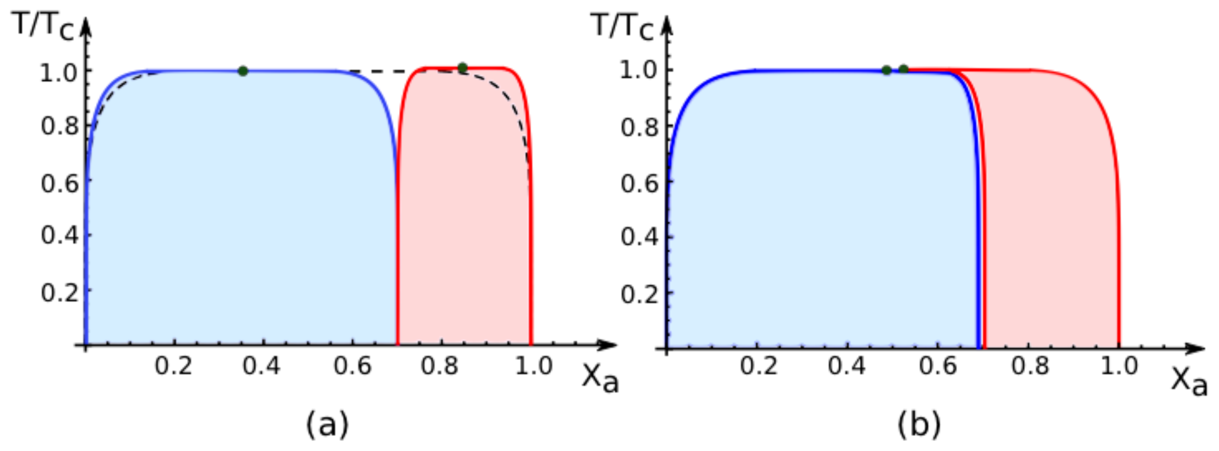
For
large positive values of the affinity contrast Δ
U2,1 as shown in
Figure 4a, the two coexistence regions differ only in their width but have the same shape. For
small positive values of
U2,1 as shown in
Figure 4b, the two coexistence regions provide a decomposition of the coexistence region of the uni-env membrane, the latter being depicted by the broken line in
Figure 4a.
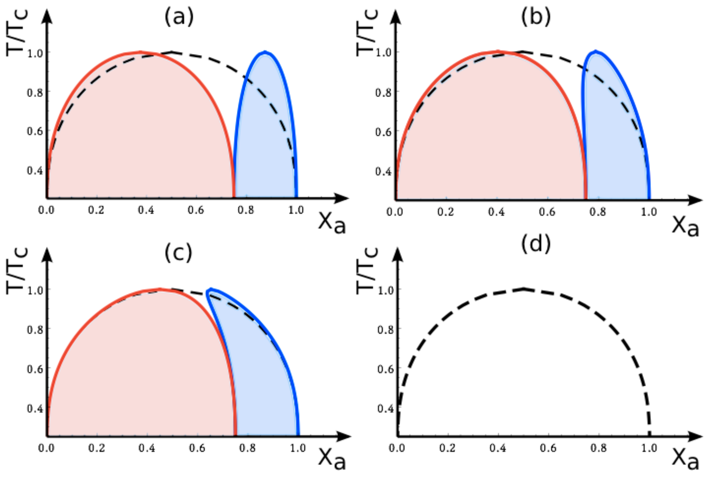
The phase diagrams in
Figure 4 correspond to fixed area fraction
. In general, this area fraction can vary in the range 0 ≤
q[1] ≤ 1. In
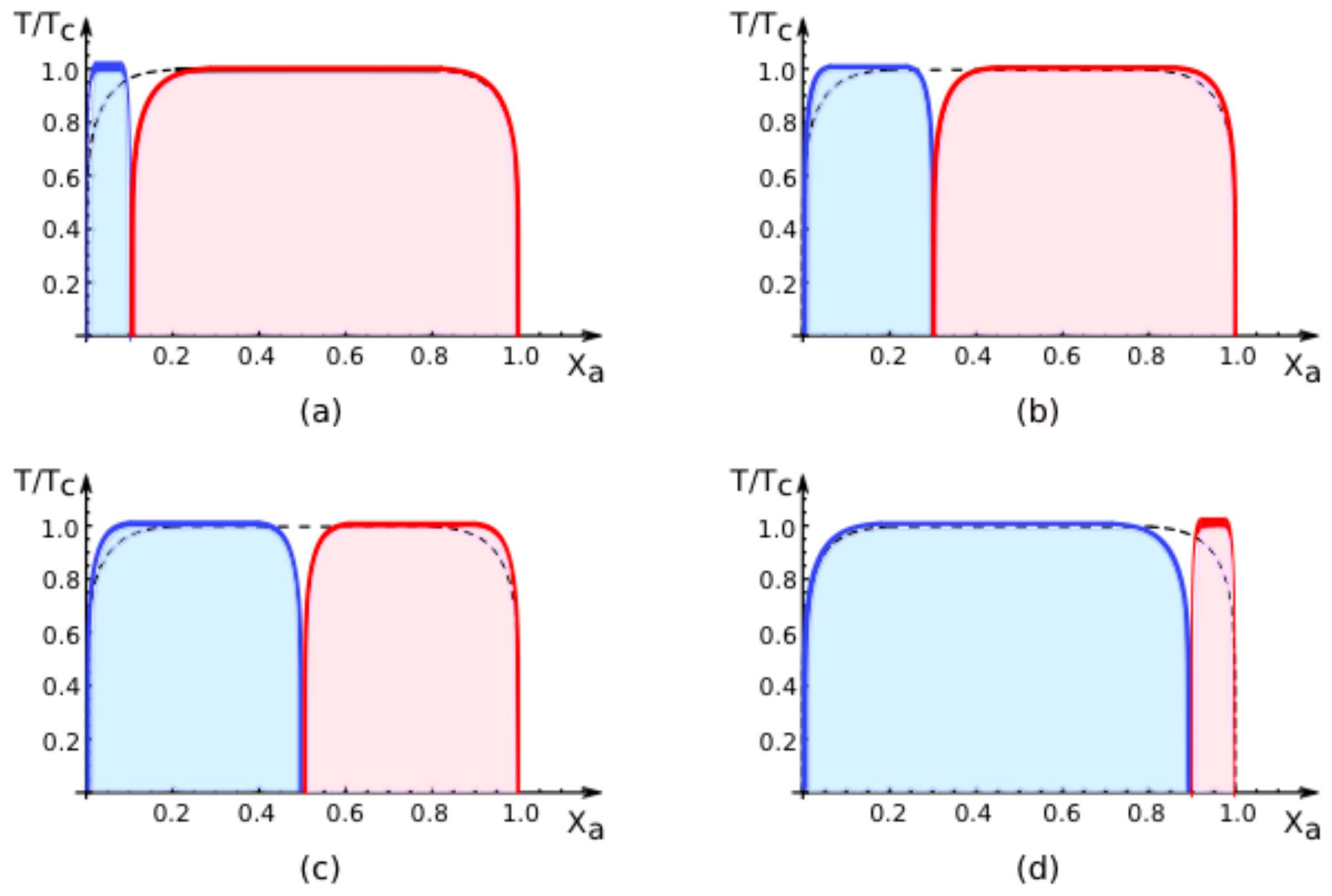
Figure 5, we show how the phase diagram evolves with increasing values of
q[1] for large, positive values of the affinity contrast Δ
U2,1. For
q[1] = 0, the adhering membrane consists of segment
only and we are left with the red coexistence region only. For small nonzero values of
q[1], a narrow blue region appears at small values of
Xa, see
Figure 5a. As we further increase the area fraction
q[1] and, thus, the relative size of segment
, the blue region grows at the expense of the red region, see
Figure 5b–d. Finally, as we reach the limiting value
q[1] = 1, the adhering membrane consists only of segment
and we are left with the blue coexistence region only. Thus, as we change the area fraction
q[1] for fixed affinity contrast Δ
U2,1, the phase diagram in the (
Xa, T/Tc)-plane evolves smoothly for all values of
q[1] including the limiting values
q[1] = 0 and
q[1] = 1. In the latter cases, we recover the coexistence region for the uni-env membrane as depicted by the broken line in
Figure 5.
All phase diagrams shown in
Figures 4 and
5 have the same topology: the single coexistence region for the uni-env membrane,
i.e., the membrane in a uniform environment, is replaced, for nonzero affinity contrast Δ
U2,1, by two coexistence regions, a blue one for segment
and a red one for segment
. For
T > 0, these two coexistence regions are separated by an intermediate one-phase region that lies within the coexistence region of the uni-env membrane. This generic topology of the phase diagrams has interesting consequences for experimental observations. Thus, consider a two-component membrane that is phase separated when exposed to a uniform environment. After this membrane is segmented by adhesion, the phase separation is restricted to one of the two membrane segments,
i.e., phase separation can be observed either in segment
or in segment
but not in both segments simultaneously. Furthermore, for mole fractions and temperatures that correspond to the intermediate one-phase regions between the two coexistence regions of the membrane segments, the phase separation in the uni-env membrane is suppressed by the adhesion-induced segmentation.
7.3. Phase Diagrams for Negative Affinity Contrasts
In
Figure 6, we display the phase diagrams of adhering membranes in the (
Xa, T/Tc)-plane as obtained from the lattice model for small and large
negative values of the affinity contrast Δ
U2,1 = Δ
U[2] − Δ
U[1] keeping the area fraction
q[1] of segment
constant. When the relative affinities Δ
U[m] are expressed in terms of the molecular interaction energies
Ua[m] and
Ub[m], we now find that
Because we use the sign convention that attractive interaction energies are negative, see (
32), the second inequality in (
68) applies to systems, in which the
a-molecules prefer to stay in segment
while the
b-molecules prefer to stay in segment
. Therefore, as one increases the mole fraction
Xa starting from
Xa = 0, the
a-molecules are first enriched in segment
, which then undergoes phase separation leading to the red coexistence regions in
Figure 6.
The phase diagrams for negative values of the affinity contrast are intimately related to those for positive values. This relation can be understood as follows. Instead of changing the sign of the affinity contrast Δ
U2,1, we could also interchange the names of the
a- and the
b-molecules. We would then obtain the same phase diagrams as in
Figures 4 and
5 but with
Xa replaced by
Xb. If we now redraw these diagrams in terms of
Xa = 1 −
Xb, we swap the relative positions of the blue and red coexistence regions and recover the phase diagrams for negative values of the affinity contrast as shown in
Figure 6.
7.4. Phase Behavior for Variable Affinity Contrasts
The variation of the area fraction
q[1] for fixed affinity contrast
U2,1 leads to a smooth evolution of the coexistence regions in the (
Xa, T/Tc)-plane as shown in
Figure 5. In contrast, the coexistence regions undergo abrupt changes as we vary the affinity contrast Δ
U2,1 from small positive to small negative values, or
vice versa, for fixed values of the area fraction
q[1].
As an example, consider the phase diagram for
small negative affinity contrasts Δ
U2,1 and
q[1] = 0.7 as shown in
Figure 6b. This phase diagram exhibits a relatively narrow red coexistence region for mole fractions
Xa in the range 0 ≲
Xa ≲ 0.3 and a relatively broad blue coexistence region for mole fractions within 0.3≲
Xa ≲ 1, separated by a very narrow one-phase region. For
vanishing affinity contrast Δ
U2,1 = 0, this one-phase region has disappeared and the red and blue regions have merged into the single coexistence region for the uni-env membrane, see broken lines in
Figures 4 and
6. Finally, for
small positive affinity contrasts Δ
U2,1, the blue and the red coexistence regions swap their relative positions: the relatively broad blue coexistence region is now located at 0 ≲
Xa ≲ 0.7 and the relatively narrow red coexistence region at 0.7 ≲
Xa ≲ 1. Thus, as we change the sign of the affinity contrast, the phase diagrams change in an abrupt and discontinuous manner.
The abrupt changes of the (
Xa, T/Tc) phase diagrams arising from variations of the affinity contrast are limited to the vicinity of Δ
U2,1 = 0. Indeed, as long as we do not cross Δ
U2,1 = 0, a continuous change of the affinity contrastΔ
U2,1 leads to a smooth variation of the two coexistence regions within the (
Xa, T/Tc)-plane. This latter property is illustrated in
Figure 7, which displays such a smooth variation for negative values of
U2,1 as obtained from the mean-field approximation to the lattice model defined in Section 5.2.
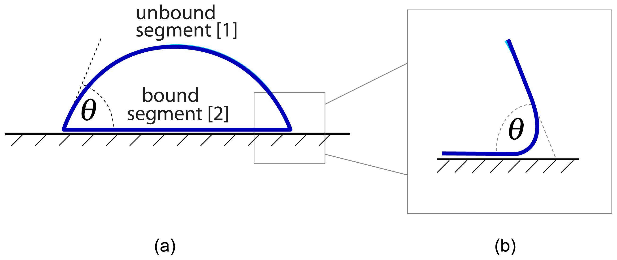
8. Summary and Outlook
In this paper, we first emphasized that the adhesion of membranes often leads to two membrane segments, denoted by
and
, that are in contact with two different environments. Examples are provided by the adhesion of vesicles, see
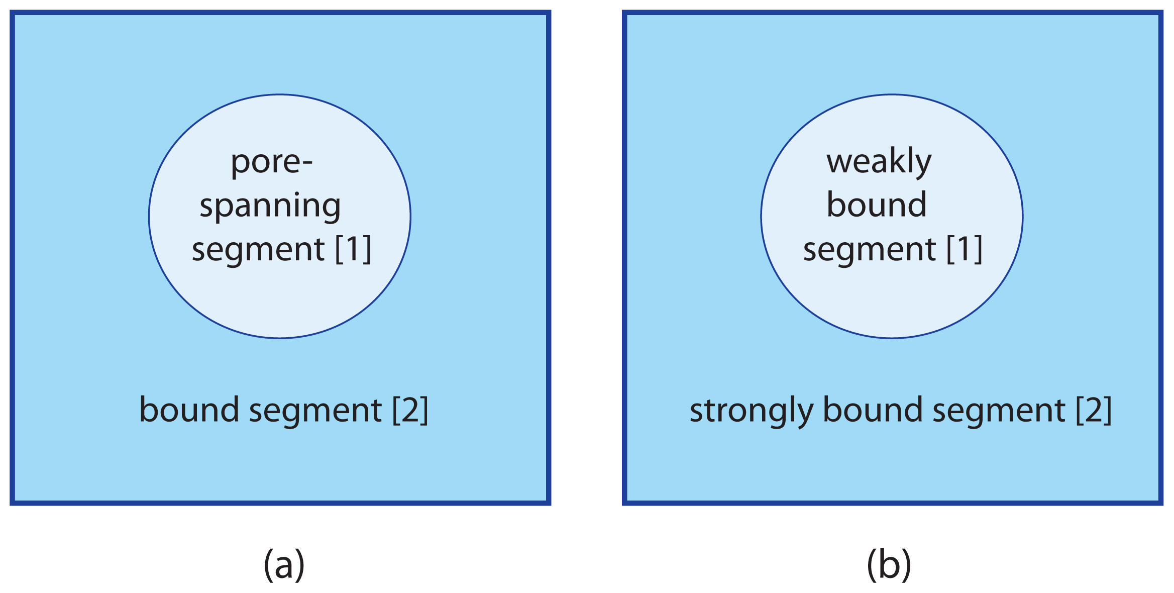
Figure 2, by hole- or pore-spanning membranes, see
Figure 3a, and by membranes supported by chemically patterned surfaces, see
Figure 3b. We then studied how these adhesion geometries affect the phase behavior of two-component membranes and vesicles.
Our theoretical analysis was based on the configurational energies
[1] and
[2] for the two membrane segments as described by the expression (
39), which generalizes the standard lattice model for binary mixtures to the different adhesion geometries considered here. In the configurational energies
[1] and
[2], the interactions of the
a- and
b-molecules with the different environments are taken into account by the relative affinities Δ
U[1] and Δ
U[2] as defined in (
33). These relative affinities shift the relative chemical potential Δ
μ =
μa −
μb for the
a- and
b-molecules within the two membrane segments. From these shifts alone, we can conclude that the two membrane segments undergo two distinct phase transitions for Δ
U[1] ≠ Δ
U[2] as follows from the relations in (
42).
In order to obtain theoretical predictions that are accessible to experiments, we then considered the mole fractions
Xa[1] and
Xa[2] in the two membrane segments and showed how these mole fractions determine the phase diagrams as a function of the overall mole fraction
Xa and the dimenionsless temperature
T̄ via the partitioning relation (
44) and the chemical equilibrium between the two membrane segments. As a result, we found that the phase behavior of the adhering membranes depends, in general, on four parameters: overall mole fraction
Xa, temperature
T̄, area fraction
q[1], and affinity contrast Δ
U2,1 = Δ
U[2] − Δ
U[1] as defined in (
49).
For the generic case of nonzero affinity contrast, the phase diagrams for the adhering membranes contain two distinct coexistence regions in the (
Xa, T̄)-plane separated by an intermediate one-phase region as shown in
Figures 4–
7. These different regions evolve smoothly as one changes one of the four parameters except for variations of the affinity contrast Δ
U2,1 across the hyperplane defined by Δ
U2,1 = 0. The latter behavior is illustrated by the phase diagrams in
Figures 4b and
6b, which correspond to small positive and small negative values of the affinity contrast, respectively.
All phase diagrams shown in
Figures 4–
7 have the same topology. This universality has interesting consequences for experimental observations. Thus, consider a two-component membrane or vesicle that is phase separated when exposed to a uniform environment. When this membrane or vesicle is brought into contact with two different environments that lead to a nonzero affinity contrast, see the examples in
Figure 2 or
Figure 3, the phase separation is confined to one of the two membrane segments,
i.e., phase separation may be observed either in segment
or in segment
but not in both segments simultaneously. Furthermore, if the mole fraction and temperature of the adhering membrane belong to the intermediate one-phase region between the two two-phase coexistence regions in the (
Xa, T̄)-plane, phase separation and domain formation are suppressed by the adhesion-induced segmentation. In this way, we predict generic features of the adhesion-induced phase behavior that can be scrutinized by experiment.
The theory described here can be extended and generalized in several ways. First, it is possible to study the dynamics of the phase separation processes, which proceed via the formation and coarsening of intramembrane domains within the two membrane segments, by simulations of the lattice model. We have already performed preliminary Monte Carlo simulations that support the phase diagrams described in this paper. Second, one can apply the theoretical approach used here for the lattice binary mixture to any two-component membrane. One exampe is provided by binary cholesterol/DPPC mixtures, for which the phase diagram in
Figure 1 has been deduced [
5,
8]. This phase diagram is primarily based on nuclear magnetic resonance measurements, which reveal intramembrane domains. In the study presented here, we adopted the view that these domains arise from phase separation into liquid-ordered and liquid-disordered phases in agreement with the latest data analysis [
5] and the recent review in [
8]. It has also been suggested that the domains may arise via different mechanisms such as enhanced composition fluctuations or the formation of molecular complexes as reviewed in [
6]. The experimental confirmation of the adhesion-induced phase behavior described here would provide rather strong evidence for domain formation via phase separation. Third, our theory can be extended to membranes in contact with an arbitrary number of environments as well as to membranes containing three or more molecular components as will be shown elsewhere.
For two-component membranes exposed to two different environments as considered here, the phase diagrams depend on four parameters, three of which are easy to determine experimentally. Indeed, the mole fraction Xa the temperature T are standard thermodynamic control parameters while the area fraction q[1] can be controlled by the design of the adhesion system. The remaining parameter provided by the affinity contrast ΔU2,1 could also be determined experimentally. For adhering vesicles, for instance, one can measure the adhesion energy of the bound membrane segment for different membrane compositions, from which the relative affinities of the bound membrane segment and, thus, the affinity contrast can be deduced. Alternatively, one may also obtain these relative affinities from molecular dynamics simulations of atomistically resolved membranes.


