3.1. Spectroscopic Parameters of Λ-S States
The Davidson modification lowers the total energy by 26.084 and 29.531 mE
h for the X
2Π and A
2Π electronic states near the internuclear equilibrium separations, respectively.
Table 1 demonstrates the effects on the
Te,
Re,
ωe and other spectroscopic parameters by the Davidson modification. As seen in
Table 1, (1) the effect on the
Te of the A
2Π electronic state by the Davidson modification is very significant. The shift of the
Te lowered by the modification is 756.53 cm
−1; (2) the Davidson modification lengthens the
Re only by 0.00019 and 0.00013 nm for the X
2Π and A
2Π electronic states, respectively; (3) the effects on the
ωe by the Davidson modification are unequal for the two electronic states. It lowers the
ωe by 5.29 cm
−1 for the X
2Π but raises the
ωe by 4.601 cm
−1 for the A
2Π electronic state. On the whole, the effects on the
Te by the Davidson modification are more pronounced than those on the
Re and
ωe.
With only the core-valence correlation correction included in the X
2Π and A
2Π electronic states, the total energies are lowered by about 353.454 and 350.428 mE
h for the MRCI and 376.023 and 373.538 mE
h for the MRCI+Q calculations near the internuclear equilibrium separation, respectively. From
Table 1, one can see that (1) the core-valence correlation correction makes the
Te of the A
2Π electronic state increase for the MRCI and MRCI+Q calculations; (2) the correlation correction shortens the
Re of the X
2Π and A
2Π electronic states. In detail, the
Re is shortened by 0.00043 and 0.00047 nm for the MRCI and 0.00039 and 0.00045 nm for the MRCI+Q calculations; (3) for the X
2Π and A
2Π electronic states, the correlation correction raises the
ωe by 10.64 and 2.201 cm
−1 for the MRCI and 9.92 and 3.152 cm
−1 for the MRCI+Q calculations. On the whole, the effects on the
Re and
ωe by the core-valence correlation correction are more pronounced than those by the Davidson modification.
With only the scalar relativistic correction added in the X
2Π and A
2Π electronic states, the total energy is lowered by about 1.135 E
h near the internuclear equilibrium position.
Table 1 collects the spectroscopic results corrected by the relativistic effect. As shown in
Table 1, (1) the scalar relativistic correction lowers the
Te of the A
2Π electronic state by 63.65 cm
−1 for the MRCI and 60.57 cm
−1 for the MRCI+Q calculations; (2) the scalar relativistic correction has a very small effect on the
Re. The largest shifts of
Re are only 0.00001 and 0.00012 nm for the X
2Π and A
2Π electronic states, respectively; (3) for the X
2Π electronic state, the scalar relativistic correction lowers the
ωe by 2.76 and 2.71 cm
−1 for the MRCI and MRCI+Q calculations. And for the A
2Π electronic state, the scalar relativistic correction lowers the
ωe by 2.087 and 1.975 cm
−1 for the MRCI and MRCI+Q calculations. Obviously, the effects on the
Te,
Re and
ωe by the scalar relativistic correction are smaller than those by the core-valence correlation correction.
With the core-valence correlation and scalar relativistic corrections included synchronously, one can find that the spectroscopic parameters are in excellent agreement with the measurements, in particular at the MRCI+Q level. For this reason, we make a brief comparison between the present results obtained by the MRCI+Q/AV5Z+DK+CV calculations and the measurements. (1) The present
Te of the A
2Π electronic state is 31429.43 cm
−1, which is smaller than the measurements [
17] by only 55.05 cm
−1; (2) Favorable agreement can be found between the present
Re results and the measurements [
17]. The deviations of the present
Re from the measurements [
17] are 0.00030 (0.21%) and 0.00021 nm (0.13%) for the X
2Π and A
2Π electronic states; (3) Excellent agreement is observed between the present
ωe and measurements. The deviations of the present
ωe from the measurements [
17] are 0.43 cm
−1 for the X
2Π and 0.94 cm
−1 for the A
2Π electronic state. (4) As shown in
Table 1, other spectroscopic parameters (
ωexe,
Be,
αe and
Drot) also agree favorably with the measurements [
17]. The comparison demonstrates that the present calculations with the core-valence correlation and scalar relativistic corrections and Davidson modification can improve the quality of spectroscopic parameters. For convenient comparison, here we collect the spectroscopic results obtained by the MRCI+Q/AV5Z +CV+DK calculations together with the available experimental [
10–
15,
17,
20] and other theoretical [
9,
24,
25] results in
Table 2.
For the X
2Π electronic state, as shown in
Table 2, no other theoretical spectroscopic parameters are superior to the present ones when compared with the measurements [
17]. In this respect, we think that the spectroscopic parameters of the SO
+(X
2Π) cation collected in
Table 2 are of high quality.
By the way, at the MRCI+Q/AV5Z+CV+DK level, we have determined the dissociation energies, 5.4010 and 3.3976 eV, for the X
2Π and A
2Π Λ-S states, respectively. The experimental dissociation energy of the X
2Π Λ-S state reported in [
49] is 5.43 ± 0.19 eV, and the experimental dissociation energy of the A
2Π Λ-S state is 3.3756 ± 0.19 eV if we employ the
Te reported in [
17]. Obviously, excellent agreement exists between the present dissociation energies and the experimental ones.
3.2. Spin-Orbit Effects in X2Π and A2Π States
For detailed comparison with available experimental and theoretical results, we study the effect on the spectroscopic parameters of the X
2Π electronic state by the spin-orbit coupling correction. Lam
et al. [
22] in 2011 used the MRCI/cc-pwCV5Z method to calculate the
A0 for the SO
+(X
2Π
1/2, 3/2). Their result, 359.0 cm
−1, is closer to the measurements [
22] than the one, 330 cm
−1, obtained by their MRCI calculations without using core-valence basis sets and all electrons (except two 1 s
2 electrons of sulfur atom) in the active space. According to their theoretical results, Lam
et al. [
22] thought that the quality of the
A0 could be improved by the additional treatment of core electrons. In addition, Lam
et al. [
22] also thought that it was premature at this point to conclude that correlating core electrons (augmented with appropriate core-valence basis sets) in the active space was a necessity for increasing the accuracy of the spin-orbit coupling calculations. To check this standpoint, here, we use two all-electron basis sets, ACVTZ and AVTZ, to perform the present spin-orbit coupling calculations. For the X
2Π
1/2, X
2Π
3/2, A
2Π
1/2 and A
2Π
3/2 Ω states, we collect the spectroscopic parameters obtained by the MRCI+Q/AV5Z+SO calculations in
Table 3, for which the AVTZ basis set is used to calculate the spin-orbit coupling corrections; and we tabulate the spectroscopic parameters obtained by the MRCI+Q/AV5Z +SO calculations in
Table 4, for which the ACVTZ basis set is used to calculate the spin-orbit coupling corrections. For convenient comparison, for the X
2Π and A
2Π Λ-S states, we present the spectroscopic parameters calculated by the MRCI+Q method in combination with the AV5Z basis set in
Tables 3 and
4, respectively, for which the spin-orbit coupling corrections are omitted.
When the AVTZ basis set is used to perform the spin-orbit coupling calculations at the MRCI+Q level, the total energy of the X
2Π
1/2 component is −472.493589 E
h, and the total energy of the X
2Π
3/2 component is −472.492020 E
h at the internuclear equilibrium position. The former is lower than and the latter is higher than the corresponding one, −472.492804 E
h, of the X
2Π electronic state. With the spin-orbit coupling correction added in the present MRCI+Q/AV5Z calculations, the energy separation of the two splitting components (X
2Π
1/2 and X
2Π
3/2) is 344.36 cm
−1. According to the potential energies given here, it is not difficult to determine that the ground-state energy is lowered by about 172.29 cm
−1 due to the spin-orbit coupling effect. As shown in
Table 3, the spin-orbit coupling correction has no effect on the
Re and only produces a very small effect on the
ωe.
When the ACVTZ basis set is used to make the spin-orbit coupling calculations at the MRCI+Q level, the total energy of the X
2Π
1/2 component is −472.829051 E
h, and the total energy of the X
2Π
3/2 component is −472.827401 E
h at the equilibrium position. At this time, the total energy of the SO
+(X
2Π) cation obtained by the MRCI+Q/ACVTZ calculations is −472.828226 E
h. From this data, it is not difficult to determine that the
A0 value of the SO
+(X
2Π
1/2, 3/2) is 361.91 cm
−1, and the ground-state energy of the cation is lowered by about 181.07 cm
−1 due to the spin-orbit coupling effect. As shown in
Table 4, the spin-orbit coupling correction has no effect on the
Re and produces a very small effect on the
ωe. For the X
2Π electronic state, by comparison, it can be concluded that the ACVTZ basis set makes the spin-orbit coupling constant
A0 of the SO
+(X
2Π
1/2, 3/2) slightly larger and closer to the measurements [
22] when compared with the one, AVTZ, for the spin-orbit coupling calculations.
Now we study the effect on the spectroscopic parameters by the spin-orbit coupling splitting when the core-valence correlation and scalar relativistic corrections are added. At this time, for the X
2Π
1/2, X
2Π
3/2, A
2Π
1/2 and A
2Π
3/2 Ω states, the spectroscopic results obtained by using the AVTZ basis set for the spin-orbit coupling calculations are presented in
Table 5. Similar to
Tables 3 and
4, here we also tabulate the spectroscopic results obtained by the MRCI+Q/AV5Z+CV+DK calculations without the spin-orbit coupling in
Table 5 as the X
2Π and A
2Π results for comparison. By comparison between
Table 3 and
5, we find that the inclusion of core-valence correlation and scalar relativistic corrections does not bring about the effect on the
A0, but makes the
Re and
ωe closer to the measurements [
12,
13].
Table 6 presents the spectroscopic parameters of the X
2Π
1/2 and X
2Π
3/2 components obtained by the MRCI+Q/AV5Z+CV+DK+SO calculations. Different from
Table 5, it should be pointed out that the spin-orbit coupling calculations in
Table 6 are performed with the core-valence correlation ACVTZ basis set. Here, we tabulate the spectroscopic parameters obtained by the MRCI+Q/AV5Z+CV+DK calculations without the spin-orbit coupling in
Table 6 as the “X
2Π” results, and we also collect some experimental [
10–
13] and theoretical [
10,
13,
23] results in
Table 6 for convenient comparison. In order to avoid congestion in
Table 6, other experimental [
14,
15,
17,
18,
20,
22] and theoretical [
9,
13,
22]
A0 values of the SO
+(X
2Π
3/2, 1/2) are presented in
Table 7. The PEC obtained by the MRCI+Q/AV5Z+CV+DK calculations of the SO
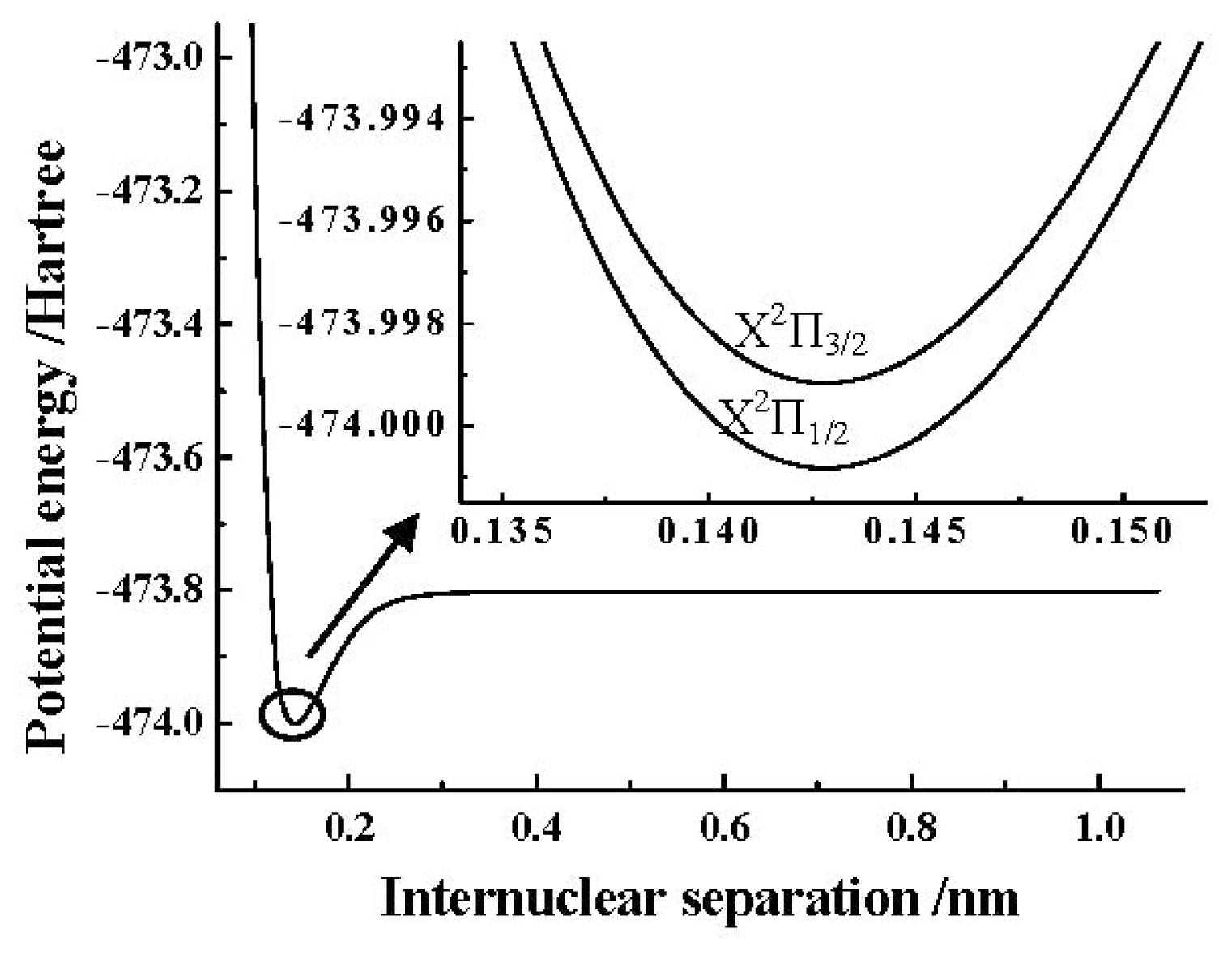
+(X
2Π) cation is depicted in
Figure 1. In addition, the detailed PECs of the SO
+(X
2Π
3/2, 1/2) components near the equilibrium position obtained by using the ACVTZ basis set for the spin-orbit coupling corrections are also shown in the same
Figure 1.
As seen in
Table 6, at the MRCI+Q/AV5Z+CV+DK+SO level, the
A0 of the SO
+(X
2Π
1/2, 3/2) obtained by using the ACVTZ basis set for the spin-orbit coupling calculations is 362.13 cm
−1, which agrees well with the recent measurements, 365.36 cm
−1 [
22]. The result is obviously superior to the one obtained by using the AVTZ basis set for the spin-orbit coupling correction. As demonstrated in
Table 7, the
A0 difference between the ACVTZ and AVTZ basis set is 17.77 cm
−1. The conclusion can also be drawn that the ACVTZ basis set makes the
A0 of the SO
+(X
2Π
1/2, 3/2) slightly larger and closer to the measurements [
22] when compared with the one, AVTZ, for the spin-orbit coupling calculations.
From
Tables 6 and
7, at the MRCI+Q/AV5Z+CV+DK+SO level, we can clearly see that the
A0 of the SO
+(X
2Π
1/2, 3/2) obtained by using the ACVTZ basis set for the spin-orbit coupling calculations is the closest to the recent measurements [
22] among all the theoretical results [
9,
10,
13,
22]. Other spectroscopic results such as
Re,
ωe and
ωexe also agree favorably with the experimental ones [
12,
13]. As a conclusion, we think that the spectroscopic parameters collected in
Table 6 are of high quality.
As shown in
Table 2, only Houria
et al. [
9] in 2006 have studied the spectroscopic parameters of the A
2Π electronic state. Obviously, the present results are superior to those obtained by Houria
et al. [
9] when compared with the measurements [
17].
At the equilibrium position, when the AVTZ basis set is used to calculate the spin-orbit coupling splitting, we find that the total energy of A
2Π
1/2 component is higher, but the total energy of A
2Π
3/2 is lower than that of the SO
+(A
2Π) cation. With the correction results added into the present MRCI+Q/AV5Z values, the obtained spectroscopic results are collected in
Table 3. As shown in
Table 3, the
A0 for the SO
+(A
2Π
3/2, 1/2) is 52.67 cm
−1, which is in excellent agreement with the experimental one, 53.88 cm
−1 [
17]. At this time, the effects on the
Re and
ωe by the spin-orbit coupling are still very small, and the separations between the A
2Π
1/2 and A
2Π
3/2 components are only 0.00001 nm for the
Re and 0.65 cm
−1 for the
ωe.
At the equilibrium position, when the ACVTZ basis set is used to calculate the spin-orbit coupling splitting, we also find that the total energy of the A
2Π
1/2 component is higher, and the total energy of A
2Π
3/2 is lower than that of the SO
+(A
2Π) cation. With these correction results added into the present MRCI+Q/AV5Z values, the obtained spectroscopic results are collected in
Table 4. As shown in
Table 4, the
A0 for the SO
+(A
2Π
3/2, 1/2) is 57.94 cm
−1, which deviates more [
22] than the one, 52.67 cm
−1, obtained by using the AVTZ basis set for the spin-orbit coupling calculations. In addition, the effects on the
Re and
ωe by the spin-orbit coupling correction are very small, and the separations between the A
2Π
3/2, 1/2 components are only 0.00003 nm for the
Re and 0.789 cm
−1 for the
ωe, respectively.
Table 5 also tabulates the spectroscopic results obtained by using the AVTZ basis set for the spin- orbit coupling calculations of the A
2Π
1/2 and A
2Π
3/2 components at the MRCI+Q/AV5Z+CV+DK level. As shown in
Table 5, the inclusion of core-valence correlation and scalar relativistic corrections brings about no effect on the
A0 for the SO
+(A
2Π
3/2, 1/2), and still produces a very small effect on the
Re and
ωe.
Table 6 demonstrates the effect on the spectroscopic results of the A
2Π
1/2 and A
2Π
3/2 components by the core-valence correlation and scalar relativistic corrections when the ACVTZ basis set is used to make the spin-orbit coupling correction calculations. One can still find that the effects on the
A0,
Re and
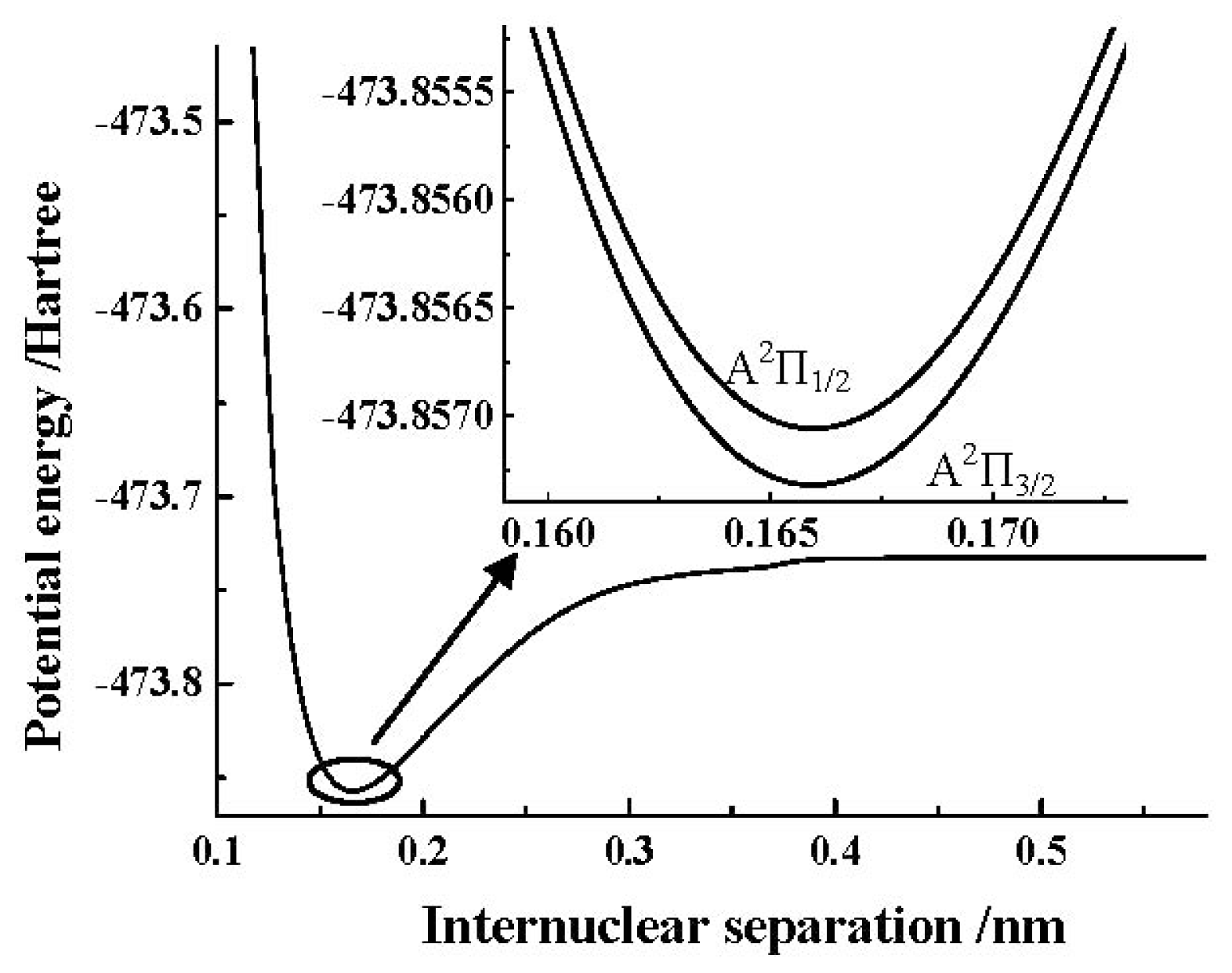
ωe by the spin-orbit coupling correction are very small. In addition, we depict the PEC obtained by the MRCI+Q/AV5Z+CV+DK calculations of the SO
+(A
2Π) cation in
Figure 2. Similar to the X
2Π Λ-S state, to clearly show the details of the spin-orbit coupling splitting, we also depict the PECs obtained by the MRCI+Q/AV5Z+CV+DK+SO calculations of SO
+(A
2Π
3/2, 1/2) components using the ACVTZ basis set for the spin-orbit coupling correction in the same
Figure 2.
As a conclusion, we think that (1) for the MRCI+Q/AV5Z+CV+DK+SO calculations, the
A0 of the SO
+(X
2Π
1/2, 3/2) obtained by the ACVTZ basis set is closest to the measurements [
22]. The
A0 of the SO
+(A
2Π
1/2, 3/2) obtained by the ACVTZ basis set also agree well with the measurements [
17], and the difference between such
A0 result and the experimental one is only several cm
−1; (2) the core-valence correlations make the
A0 become large for the two electronic states but are not sure to increase the accuracy of the spin-orbit coupling constant
A0; (3) the spectroscopic results determined by the MRCI+Q/AV5Z+CV+DK calculations for the X
2Π and A
2Π electronic states have achieved a high quality.
3.3. Vibrational Manifolds
Here, we only use the PECs obtained by the MRCI+Q/AV5Z+DK+CV calculations to determine the vibrational manifolds of X
2Π and A
2Π electronic states. The reason is that no spin-orbit coupling experimental
G(
υ),
Bυ and
Dυ values exist in the literature, whereas the corresponding results can be found for the X
2Π and A
2Π electronic states. The vibrational level
G(
υ), inertial rotation constant
Bυ and centrifugal distortion constant
Dυ are predicted for each vibrational state of each electronic state by solving the ro-vibrational Schrödinger equation of nuclear motion using Numerov’s method [
43]. Due to length limitation, here we only tabulate the
G(
υ),
Bυ and
Dυ results of the first 30 vibrational states of SO
+(X
2Π) and SO
+(A
2Π) cation for the
J = 0 case in
Tables 8 and
9, respectively.
For the
G(
υ) of X
2Π electronic state, only one group of RKR data can be found in the literature [
49]. We collect the only group of RKR data in
Table 8 for comparison. As seen in
Table 8, excellent agreement exists between them. For example, the deviations of the present
G(
υ) results from the RKR data [
49] is only 0.29, 3.67, 6.45 and 8.97 cm
−1 for
υ = 0, 6, 10 and 16, respectively.
At least four groups of
Bυ experimental data exist in the literature [
15–
17,
21] for the SO
+(X
2Π) cation. In order to avoid congestion in
Table 8, here we only tabulate the
Bυ given by Hardwick
et al. [
15], Milkman
et al. [
16] and Dyke
et al. [
21] for comparison. As demonstrated in
Table 8, the present
Bυ are in excellent agreement with all the measurements [
15,
16,
21] collected in
Table 1. For example, the largest deviation of the present
Bυ results from the measurements [
15] is 0.34% (which corresponds to
υ = 4). The largest deviation of the present
Bυ results from the measurements [
16] is 0.373% (which corresponds to
υ = 4). And the largest deviation of the present
Bυ results from the measurements [
21] is 0.34%. When we compare the present
Bυ with those [
17] not collected in
Table 8, good accord also exists between them. Therefore, we think, with reason, that the newly calculated
Bυ results are of a very high quality.
Similar to the
Bυ, there are also four groups of measurements [
15–
17,
21] and one group of RKR data [
17] concerning the
Dυ of the SO
+(X
2Π) cation. To avoid congestion in
Table 8, we only tabulate three groups of measurements [
15,
16,
21] and one group of RKR data in the table. It is not difficult to find that excellent agreement exists between the present results and the measurements [
15,
16] as well as RKR data [
17]. For example, the present results are smaller than the measurements [
15] only by 0.79% and 3.85% for
υ = 4 and 5, and the present results are smaller than the experimental data [
21] also only by 0.76% and 1.74% for
υ = 0 and 1, respectively. Because the
Dυ is a very small quantity, such deviation is acceptable. In addition, when we compare the experimental
Dυ results [
17] not collected in
Table 8, excellent agreement can also be found between them.
Table 9 collects the present
G(
υ),
Bυ and
Dυ results of the
32S
16O
+(A
2Π) cation until
υ = 29 together with three groups of measurements [
15–
17]. From
Table 9, we can see that the difference between the G(0) and G(1) is equal to 792.2 cm
−1, whereas the corresponding experimental difference obtained by Coxon and Foster [
14] is 792.7 cm
−1. Excellent agreement exists between the present result and the experimental one. As seen in
Table 9, the present
Bυ results agree favorably with the measurements [
15–
17]. For example, the differences between the present
Bυ results and the measurements [
15] are only 0.17% and 0.19% for
υ = 0 and 1, and the differences between the present
Bυ and the measurements [
16] are 0.12%, 0.30%, 0.04% and 0.49% for
υ = 0, 4, 7 and 11, respectively. At the same time, the largest deviation of the present
Bυ results from the measurements [
17] is also only by 0.29% (which corresponds to
υ = 5). All the comparisons demonstrate that the present
Bυ results tabulated in
Table 9 are accurate.
As for the
Dυ results of the
32S
16O
+(A
2Π) cation, three groups of experimental results [
15–
17] and one group of RKR data [
17] have been found in the literature to our knowledge. For convenient comparison with the present results and to avoid congestion, only some of these experimental data are collected in
Table 9. As seen in
Table 9, excellent agreement with the measurements [
15,
16] and the RKR data [
17] still exists. For example, the largest deviation of the present
Dυ from the measurements [
15] is only by 0.60%, and the differences between the present
Dυ and the RKR data [
17] are also only 0.31%, 0.23%, 0.74% and 0.56% for
υ = 0, 4, 7 and 11, respectively. As noted above, the
Dυ is a very small quantity. Anyway, such deviation is still very small.
To the best of our knowledge, no
G(
υ) results can be found in the literature for the
32S
16O
+(A
2Π) ion, either theoretically or experimentally. Therefore, we cannot make any direct comparison between them. On the one hand, as seen in
Tables 2 and
6, the present spectroscopic parameters obtained by the MRCI+Q/AV5Z+CV+DK calculations agree well with the measurements for the two electronic states. On the other hand, the vibrational manifolds of the ground state and the
Bυ and
Dυ results of the A
2Π electronic state are also in excellent agreement with the experimental data. Because all the results are calculated by the same approach and fitted by the same procedure, we believe that the
G(
υ) results of the A
2Π electronic state collected in
Table 9 and the vibrational manifolds for higher vibrational levels presented in
Tables 8 and
9 are reliable and accurate. They should be of considerable value for future experimental or theoretical research.
Finally, we will discuss the effect on the vibrational manifolds by the spin-orbit coupling correction [
50–
53]. On the whole, the spin-orbit coupling correction brings about only small change for lower
G(
υ), whereas it can produce the shift of more than ten cm
−1 for higher
G(
υ). For example for the X
2Π electronic state, the
G(3) is 3,218.42 cm
−1 for the X
2Π
1/2 and 4,476.08 cm
−1 for the X
2Π
3/2, respectively, which deviate from the
G(3) only by 1.35 cm
−1. And the
G(29) is 31,682.47 cm
−1 for the X
2Π
1/2 and 31,644.37 cm
−1 for the X
2Π
3/2, respectively, which deviate from the
G(29) by 19.07 cm
−1.


