Predicting Complexation Thermodynamic Parameters of β-Cyclodextrin with Chiral Guests by Using Swarm Intelligence and Support Vector Machines


Abstract
:
1. Introduction
2. Methodology
2.1. Support Vector Machines Based QSPR Model
2.2. Particle Swarm Optimization
- Initialize a population of I particles with random positions and velocities in D dimensions.
- Evaluate the desired optimization function in D variables for each particle.
- Compare the evaluation with the particle’s previous best value, pbest[i]. If the current value is better than pbest[i], then pbest[i] = current value and the pbest location, pbestx[i][d], is set to the current location in d-dimensional space.
- Compare the evaluation with the swarm’s previous best value, (pbest[gbest]). If the current value is better than pbest[gbest]), then gbest = current particle’s array index.
- Change the velocity and position of the particle according to the following equations, respectively:
- Loop to step 2 until a stopping criterion, a sufficiently good evaluation function value, or a maximum number of iterations, is met.
2.3. Chiral Guest Dataset and Descriptor Generation
2.4. QSPR Models
3. Results and Discussion
4. Conclusions
Acknowledgments
References
- Szejtli, J. Introduction and general overview of cyclodextrin chemistry. Chem. Rev 1998, 98, 1743–1754. [Google Scholar]
- Lipkowitz, KB. Applications of computational chemistry to the study of cyclodextrins. Chem. Rev 1998, 98, 1829–1874. [Google Scholar]
- Estrada, E; Perdomo-Lopez, I; Torres-Labandeira, JJ. Combination of 2D-, 3D-connectivity and quantum chemical descriptors in QSPR. Complexation of α- and β-cyclodextrin with benzene derivatives. J. Chem. Inf. Comput. Sci 2001, 41, 1561–1568. [Google Scholar]
- Klein, CT; Polheim, D; Viernstein, H; Wolschann, P. Predicting the free energies of complexation between cyclodextrins and guest molecules: linear versus nonlinear models. Pharm. Res 2000, 17, 358–365. [Google Scholar]
- Klein, CT; Polheim, D; Viernstein, H; Wolschann, P. A method for predicting the free energies of complexation between β-cyclodextrin and guest molecules. J. Incl. Phenom. Macroc. Chem 2000, 36, 409–423. [Google Scholar]
- Katritzky, AR; Fara, DC; Yang, H; Karelson, M; Suzuki, T; Solovev, VP; Varnek, A. Quantitative structure-property relationship modeling of β-cyclodextrin complexation free energies. J. Chem. Inf. Comput. Sci 2004, 44, 529–541. [Google Scholar]
- Suzuki, T. A nonlinear group contribution method for predicting the free energies of inclusion complexation of organic molecules with α- and β-cyclodextrins. J Chem Inf Comput Sci 2001, 41, 1266–1273. [Google Scholar]
- Suzuki, T; Ishida, M; Fabian, WMF. Classical QSAR and comparative molecular field analyses of the host-guest interaction of organic molecules with cyclodextrins. J. Comput. -Aided Mol. Des 2000, 14, 669–678. [Google Scholar]
- Jimenez, V; Alderete, JB. The role of charge transfer interactions in the inclusion complexation of anionic guests with α-cyclodextrins. Tetrahedron 2005, 61, 5449–5456. [Google Scholar]
- Lei, L; Wen-Guang, L; Qing-Xiang, G. Association constant prediction for the inclusion of α-cyclodextrin with benzene derivatives by an artificial neural network. J. Incl. Phenom. Macroc. Chem 1999, 34, 291–298. [Google Scholar]
- Loukas, YL. Quantitative structure-binding relationships QSBR, and artificial neural networks, improved predictions in drug, cyclodextrin inclusion complexes. J. Pharm. Sci 2001, 226, 207–211. [Google Scholar]
- Bodor, N; Buchwald, P. Theoretical Insights into the formation; structure; and energetics of some cyclodextrin complexes. J. Incl. Phenom. Macroc. Chem 2002, 44, 9–14. [Google Scholar]
- Buchwald, P. Complexation Thermodynamic of cyclodextrins in the framework of a molecular size-based model for nonassociative organic liquids that includes a modified hydration-shell hydrogen-bond model for water. J. Phys. Chem. B 2002, 106, 6864–6870. [Google Scholar]
- Faucci, MT; Melani, F; Mura, P. Computer-aided molecular modeling techniques for predicting the stability of drug-cyclodextrin inclusion complexes in aqueous solution. Chem. Phys. Lett 2002, 358, 383–390. [Google Scholar]
- Hyunmyung, K; Karpjoo, J; Hyungwoo, P; Seunho, J. Preference prediction for the stable inclusion complexes between cyclodextrins and monocyclic insoluble chemicals based on Monte Carlo docking simulations. J. Incl. Phenom. Macroc. Chem 2006, 54, 165–170. [Google Scholar]
- Youngjin, C; Kum, WC; Karpjoo, J; Seung, RP; Seunho, J. Computational prediction for the slopes of AL-type phase solubility curves of organic compounds complexed with α-; β-; or γ-cyclodextrins based on Monte Carlo docking simulations. J Incl Phenom Macroc Chem 2006, 55, 103–108. [Google Scholar]
- Zhao, L; Orton, E; Vemuri, NM. Predicting solubility in multiple nonpolar drugs-cyclodextrin system. J. Pharm. Sci 2002, 91, 2301–2306. [Google Scholar]
- Chari, R; Qureshi, F; Moschera, J; Tarantino, R; Kalonia, D. Development of improved empirical models for estimating the binding constant of a β-cyclodextrin inclusion complex. Pharm. Res 2009, 26, 161–171. [Google Scholar]
- Kennedy, J; Eberhart, R. Particle swarm optimization. In Proceedings of IEEE International Conference on Neural Networks; Perth, Australia, 1995; Institute of Electrical and Electronics Engineers: Piscataway, NJ, USA, 1995; Volume 4, pp. 1942–1948.
- Vapnik, V. The Nature of Statistical Learning Theory; Springer: New York, NY, USA, 1995. [Google Scholar]
- Lawtrakul, L; Prakasvudhisarn, C. Correlation studies of HEPT derivatives using swarm intelligence and support vector machines. Monatsh. Chem 2005, 136, 1681–1691. [Google Scholar]
- Joachims, T. Making large-scale support vector machine learning practical. In Advances in Kernel Methods: Support Vector Learning; Schölkopf, B, Burges, CJC, Smola, AJ, Eds.; MIT Press: Cambridge, Massachusetts, USA, 1999; pp. 169–184. [Google Scholar]
- Platt, J. Fast training of support vector machines using sequential minimal optimization. In Advances in Kernel Methods: Support Vector Learning; Schölkopf, B, Burges, CJC, Smola, AJ, Eds.; MIT Press: Cambridge, Massachusetts, USA, 1999; pp. 185–208. [Google Scholar]
- Sutter, JM; Dixon, SL; Jurs, PC. Automated descriptor selection for quantitative structure-activity relationships using generalized simulated annealing. J. Chem. Inf. Comput. Sci 1995, 35, 77–84. [Google Scholar]
- So, SS; Karplus, M. Evolutionary optimization in quantitative structure – activity relationship: an application of genetic neural networks. J. Med. Chem 1996, 39, 1521–1530. [Google Scholar]
- Yasri, A; Hartsough, D. Toward an optimal procedure for variable selection and QSAR model building. J. Chem. Inf. Comput. Sci 2001, 41, 1218–1227. [Google Scholar]
- Hasegawa, K; Miyashita, Y; Funatsu, K. GA strategy for variable selection in QSAR studies: GA-based PLS analysis of calcium channel antagonists. J. Chem. Inf. Comput. Sci 1997, 37, 306–310. [Google Scholar]
- Agrafiotis, DK; Cedeño, W. Feature selection for structure – activity correlation using particle swarms. J. Med. Chem 2002, 45, 1098–1107. [Google Scholar]
- Eberhart, RC; Shi, Y. Particle swarm optimization: developments, applications and resources. In Proceedings of the 2001 Congress on Evolutionary Computation; Seoul, South Korea, 2001; Institute of Electrical and Electronics Engineers: Piscataway, NJ, USA, 2001; Volume 1, pp. 81–86.
- Rekharsky, MV; Inoue, Y. Chiral recognition thermodynamic of β-cyclodextrin: The thermodynamic origin of enantioselectivity and the enthalpy entropy compensation effect. J. Am. Chem. Soc 2000, 122, 4418–4435. [Google Scholar]
- Frisch, MJ; Trucks, GW; Schlegel, HB; Scuseria, GE; Robb, MA; Cheeseman, JR; Montgomery, JA, Jr; Vreven, T; Kudin, KN; Burant, JC; Millam, JM; Iyengar, SS; Tomasi, J; Barone, V; Mennucci, B; Cossi, M; Scalmani, G; Rega, N; Petersson, GA; Nakatsuji, H; Hada, M; Ehara, M; Toyota, K; Fukuda, R; Hasegawa, J; Ishida, M; Nakajima, T; Honda, Y; Kitao, O; Nakai, H; Klene, M; Li, X; Knox, JE; Hratchian, HP; Cross, JB; Bakken, V; Adamo, C; Jaramillo, J; Gomperts, R; Stratmann, RE; Yazyev, O; Austin, AJ; Cammi, R; Pomelli, C; Ochterski, JW; Ayala, PY; Morokuma, K; Voth, GA; Salvador, P; Dannenberg, JJ; Zakrzewski, VG; Dapprich, S; Daniels, AD; Strain, MC; Farkas, O; Malick, DK; Rabuck, AD; Raghavachari, K; Foresman, JB; Ortiz, JV; Cui, Q; Baboul, AG; Clifford, S; Cioslowski, J; Stefanov, BB; Liu, G; Liashenko, A; Piskorz, P; Komaromi, I; Martin, RL; Fox, DJ; Keith, T; Al-Laham, MA; Peng, CY; Nanayakkara, A; Challacombe, M; Gill, PMW; Johnson, B; Chen, W; Wong, MW; Gonzalez, C; Pople, JA. Gaussian 03. Gaussian, Inc: Wallingford, CT, USA, 2004. [Google Scholar]
- Molecular Operating Environment (MOE). Chemical Computing Group, Inc.: Montreal, Quebec, Canada, 2005; Available online: http://www.chemcomp.com (accessed Jul. 31, 2008).
- Lawtrakul, L; Wolschann, P; Prakasvudhisarn, C. Predicting complexation thermodynamic of β-cyclodextrin with enantiomeric pairs of chiral guests by using swarm intelligence and support vector machines. In Proceedings of the 14th International Cyclodextrins Symposium; Kyoto, Japan, 2008; The Society of Cyclodextrins, Japan: Tokyo, Japan, 2008; pp. 421–424.

| cmp | guest | Experimental | Calculation b | ||||||
|---|---|---|---|---|---|---|---|---|---|
| ln K | ΔG° | ΔH° | TΔS° | ln K | ΔG° | ΔH° | TΔS° | ||
| 1 | N-acetyl-D-phenylalanine | 4.11 | −10.18 | −8.14 | 2.04 | 4.43 | −11.61 | −8.82 | 0.78 |
| 2 | N-acetyl-L-phenylalanine | 4.21 | −10.44 | −8.17 | 2.27 | 4.43 | −11.61 | −8.82 | 0.78 |
| 3 | N-acetyl-D-tryptophan | 2.54 | −6.30 | −25.50 | −19.20 | 2.54 | −6.94 | −24.09 | −17.72 |
| 4a | N-acetyl-L-tryptophan | 2.84 | −7.04 | −23.80 | −16.80 | 2.54 | −6.94 | −24.09 | −17.72 |
| 5 | N-acetyl-D-tyrosine | 4.83 | −11.97 | −16.70 | −4.70 | 4.65 | −11.48 | −15.77 | −3.92 |
| 6 | N-acetyl-L-tyrosine | 4.87 | −12.07 | −17.10 | −5.00 | 4.65 | −11.48 | −15.77 | −3.92 |
| 7 | (1R,2S)-2-amino-1,2-diphenylethanol | 4.01 | −9.90 | −10.00 | −0.10 | 3.84 | −9.35 | −10.11 | 0.65 |
| 8a | (1S,2R)-2-amino-1,2-diphenylethanol | 3.83 | −9.50 | −10.00 | −0.50 | 3.84 | −9.35 | −10.11 | 0.65 |
| 9 | (R)-benzyl glycidyl ether | 5.46 | −13.52 | −9.20 | 4.30 | 5.21 | −13.45 | −9.58 | 4.22 |
| 10 | (S)-benzyl glycidyl ether | 5.43 | −13.50 | −9.30 | 4.20 | 5.21 | −13.45 | −9.58 | 4.22 |
| 11 | 2,3-O-benzylidene-D-threitol | 4.76 | −11.81 | −7.56 | 4.25 | 4.70 | −12.05 | −7.98 | 3.30 |
| 12 | 2,3-O-benzylidene-L-threitol | 4.74 | −11.76 | −7.49 | 4.27 | 4.70 | −12.05 | −7.98 | 3.30 |
| 13a | (2R,3R)-3-benzyloxy-1,2,4-butanetriol | 4.42 | −10.95 | −8.07 | 2.90 | 4.79 | −10.23 | −7.23 | 2.90 |
| 14 | (2S,3S)-3-benzyloxy-1,2,4-butanetriol | 4.44 | −11.01 | −7.79 | 3.20 | 4.79 | −10.23 | −7.23 | 2.90 |
| 15 | O-benzyl-D-serine | 4.26 | −10.57 | −8.90 | 1.70 | 4.25 | −9.67 | −9.46 | 2.74 |
| 16a | O-benzyl-L-serine | 4.23 | −10.50 | −9.20 | 1.30 | 4.25 | −9.67 | −9.46 | 2.74 |
| 17 | N-t-Boc-D-alanine | 5.97 | −14.80 | −9.70 | 5.10 | 6.11 | −14.00 | −9.94 | 5.16 |
| 18 | N-t-Boc-L-alanine | 5.91 | −14.64 | −9.80 | 4.80 | 6.11 | −14.00 | −9.94 | 5.16 |
| 19 | N-t-Boc-D-alanine methyl ester | 6.49 | −16.09 | −13.82 | 2.30 | 6.40 | −14.95 | −12.37 | 2.43 |
| 20 | N-t-Boc-L-alanine methyl ester | 6.36 | −15.77 | −12.80 | 3.00 | 6.40 | −14.95 | −12.37 | 2.43 |
| 21a | N-t-Boc-D-serine | 5.72 | −14.19 | −11.00 | 3.20 | 5.33 | −13.67 | −11.20 | 2.95 |
| 22 | N-t-Boc-L-serine | 5.65 | −14.01 | −10.60 | 3.40 | 5.33 | −13.67 | −11.20 | 2.95 |
| 23 | (R)-3-bromo-8-camphorsulfonic acid | 8.23 | −20.41 | −30.10 | −9.70 | 8.03 | −19.49 | −29.63 | −9.67 |
| 24a | (S)-3-bromo-8-camphorsulfonic acid | 8.20 | −20.32 | −29.60 | −9.30 | 8.03 | −19.49 | −29.63 | −9.67 |
| 25 | (R)-3-bromo-2-methyl-1 propanol | 4.96 | −12.29 | −9.30 | 3.00 | 4.97 | −12.47 | −10.07 | 2.65 |
| 26 | (S)-3-bromo-2-methyl-1 propanol | 4.94 | −12.25 | −10.10 | 2.20 | 4.97 | −12.47 | −10.07 | 2.65 |
| 27 | (R)-3-bromo-2-methylpropionic acid methyl ester | 5.58 | −13.80 | −12.05 | 1.80 | 5.50 | −13.90 | −12.45 | 2.40 |
| 28 | (S)-3-bromo-2-methylpropionic acid methyl ester | 5.60 | −13.90 | −12.40 | 1.50 | 5.50 | −13.90 | −12.45 | 2.40 |
| 29a | (R)-camphanic acid | 5.18 | −12.85 | −17.80 | −5.00 | 5.23 | −15.01 | −19.07 | −6.17 |
| 30 | (S)-camphanic acid | 5.33 | −13.22 | −17.70 | −4.50 | 5.23 | −15.01 | −19.07 | −6.17 |
| 31 | (1R,3S)-camphoric acid | 2.94 | −7.30 | −15.50 | −8.20 | 3.02 | −8.52 | −13.02 | −6.63 |
| 32a | (1S,3R)-camphoric acid | 3.18 | −7.90 | −8.30 | −0.40 | 3.02 | −8.52 | −13.02 | −6.63 |
| 33 | (R)-camphorquinone-3-oxime | 7.87 | −19.50 | −27.10 | −7.60 | 7.62 | −19.33 | −27.04 | −6.91 |
| 34 | (S)-camphorquinone-3-oxime | 7.80 | −19.34 | −27.20 | −7.90 | 7.62 | −19.33 | −27.04 | −6.91 |
| 35 | (R)-10-camphorsulfonic acid | 6.34 | −15.70 | −20.70 | −5.00 | 6.46 | −15.44 | −20.53 | −5.74 |
| 36 | (S)-10-camphorsulfonic acid | 6.19 | −15.35 | −19.50 | −4.20 | 6.46 | −15.44 | −20.53 | −5.74 |
| 37a | N-Cbz-D-alanine | 5.00 | −12.40 | −8.90 | 3.50 | 4.81 | −12.64 | −8.69 | 2.17 |
| 38 | N-Cbz-L-alanine | 4.99 | −12.37 | −10.00 | 2.40 | 4.81 | −12.64 | −8.69 | 2.17 |
| 39 | (1R,2R)-trans-1,2-cyclohexanediol | 4.44 | −11.01 | −3.98 | 7.03 | 4.66 | −12.04 | −4.54 | 7.43 |
| 40a | (1S,2S)-trans-1,2-cyclohexanediol | 4.45 | −11.04 | −4.21 | 6.83 | 4.66 | −12.04 | −4.54 | 7.43 |
| 41 | (R)-1-cyclohexylethylamine | 5.80 | −14.37 | −7.85 | 6.50 | 5.59 | −14.24 | −7.94 | 6.15 |
| 42 | (S)-1-cyclohexylethylamine | 5.79 | −14.36 | −7.87 | 6.50 | 5.59 | −14.24 | −7.94 | 6.15 |
| 43 | O,O'-dibenzoyl-D-tartaric acid | 3.47 | −8.60 | −7.00 | 1.60 | 3.39 | −7.95 | −6.32 | 2.02 |
| 44 | O,O'-dibenzoyl-L-tartaric acid | 3.00 | −7.40 | −4.90 | 2.50 | 3.39 | −7.95 | −6.32 | 2.02 |
| 45a | Gly-D-Phe | 3.85 | −9.54 | −7.93 | 1.60 | 3.96 | −10.44 | −11.79 | 1.74 |
| 46 | Gly-L-Phe | 3.99 | −9.89 | −8.59 | 1.30 | 3.96 | −10.44 | −11.79 | 1.74 |
| 47 | (R)-hexahydromandelic acid | 6.47 | −16.05 | −5.61 | 10.44 | 6.11 | −14.54 | −5.92 | 9.37 |
| 48a | (S)-hexahydromandelic acid | 6.40 | −15.87 | −5.36 | 10.51 | 6.11 | −14.54 | −5.92 | 9.37 |
| 49 | (1R,2R,5R)-2-hydroxy-3-pipanone | 7.77 | −19.30 | −19.50 | −0.20 | 8.05 | −19.47 | −19.79 | −1.12 |
| 50 | (1S,2S,5S)-2-hydroxy-3-pipanone | 7.75 | −19.20 | −20.00 | −0.80 | 8.05 | −19.47 | −19.79 | −1.12 |
| 51 | (R)-mandelic acid | 2.40 | −5.90 | −4.90 | 1.00 | 2.20 | −5.63 | −5.17 | 1.11 |
| 52 | (S)-mandelic acid | 2.20 | −5.40 | −4.60 | 0.80 | 2.20 | −5.63 | −5.17 | 1.11 |
| 53a | (R)-mandelic acid methyl ester | 4.20 | −10.42 | −7.80 | 2.60 | 4.13 | −10.17 | −6.94 | −0.86 |
| 54 | (S)-mandelic acid methyl ester | 4.28 | −10.60 | −8.20 | −2.40 | 4.13 | −10.17 | −6.94 | −0.86 |
| 55 | (R)-α-methoxyphenylacetic acid | 2.40 | −5.90 | −4.40 | 1.50 | 2.79 | −7.68 | −6.63 | 1.75 |
| 56a | (S)-α-methoxyphenylacetic acid | 2.30 | −5.70 | −5.10 | 0.60 | 2.79 | −7.68 | −6.63 | 1.75 |
| 57 | (R)-α-methoxy-α-trifluoromethylphenylacetic acid | 5.16 | −12.80 | −17.48 | −4.70 | 5.45 | −13.14 | −16.92 | −4.19 |
| 58 | (S)-α-methoxy-α-trifluoromethylphenylacetic acid | 4.95 | −12.27 | −16.35 | −4.10 | 5.45 | −13.14 | −16.92 | −4.19 |
| 59 | D-phenylalanine amide | 4.62 | −11.44 | −10.00 | 1.40 | 4.66 | −11.71 | −10.01 | 0.87 |
| 60 | L-phenylalanine amide | 4.69 | −11.63 | −10.60 | 1.00 | 4.66 | −11.71 | −10.01 | 0.87 |
| 61a | D-phenylalanine methyl ester | 2.40 | −5.90 | −5.60 | 0.30 | 3.16 | −7.07 | −3.56 | 0.58 |
| 62 | L-phenylalanine methyl ester | 2.48 | −6.20 | −5.00 | 1.20 | 3.16 | −7.07 | −3.56 | 0.58 |
| 63 | (R)-2-phenylbutyric acid | 4.54 | −11.26 | −9.79 | 1.50 | 4.77 | −12.20 | −9.15 | 1.81 |
| 64a | (S)-2-phenylbutyric acid | 4.55 | −11.29 | −9.91 | 1.40 | 4.77 | −12.20 | −9.15 | 1.81 |
| 65 | (R)-3-phenylbutyric acid | 6.00 | −14.86 | −8.62 | 6.24 | 5.22 | −14.41 | −8.72 | 5.34 |
| 66 | (S)-3-phenylbutyric acid | 6.06 | −15.03 | −8.68 | 6.35 | 5.22 | −14.41 | −8.72 | 5.34 |
| 67 | (R)-1-phenyl-1,2-ethanediol | 4.13 | −10.23 | −7.54 | 2.69 | 3.85 | −9.42 | −6.96 | 2.24 |
| 68 | (S)-1-phenyl-1,2-ethanediol | 4.14 | −10.26 | −7.30 | 2.96 | 3.85 | −9.42 | −6.96 | 2.24 |
| 69a | (R)-phenyllactic acid | 4.48 | −11.10 | −9.34 | 1.80 | 5.06 | −10.83 | −8.09 | 2.99 |
| 70 | (S)-phenyllactic acid | 4.42 | −10.95 | −8.65 | 2.30 | 5.06 | −10.83 | −8.09 | 2.99 |
| 71 | (R)-2-phenylpropionic acid | 3.53 | −8.74 | −8.81 | −0.10 | 4.06 | −8.72 | −8.84 | 1.18 |
| 72a | (S)-2-phenylpropionic acid | 3.58 | −8.88 | −8.69 | 0.20 | 4.06 | −8.72 | −8.84 | 1.18 |
| 73 | (1R,2R,3S,5R)-pinanediol | 8.77 | −21.74 | −20.40 | 1.30 | 8.67 | −21.18 | −20.19 | 2.03 |
| 74 | (1S,2S,3R,5S)-pinanediol | 8.76 | −21.71 | −20.30 | 1.40 | 8.67 | −21.18 | −20.19 | 2.03 |
| SVMs | ln K | ΔG° | ΔH° | TΔS° | ||||
|---|---|---|---|---|---|---|---|---|
| R2Training | R2Testing | R2Training | R2Testing | R2Training | R2Testing | R2Training | R2Testing | |
| Linear | 0.8201 | 0.6666 | 0.8239 | 0.6349 | 0.9048 | 0.8455 | 0.8220 | 0.8257 |
| Polynomial | 0.9993 | 0.7358 | 0.9994 | 0.8213 | 0.9992 | 0.8432 | 0.9991 | 0.8251 |
| Gaussian RBF | 0.9983 | 0.9762 | 0.9987 | 0.9713 | 0.9983 | 0.9350 | 0.9986 | 0.8853 |
| Number of descriptors | ln K | ΔG° | ΔH° | TΔS° | ||||
|---|---|---|---|---|---|---|---|---|
| R2Training | R2Testing | R2Training | R2Testing | R2Training | R2Testing | R2Training | R2Testing | |
| 8 | 0.9983 | 0.9762 | 0.9987 | 0.9713 | 0.9983 | 0.9350 | 0.9986 | 0.8853 |
| 7 | 0.9977 | 0.9534 | 0.9981 | 0.9778 | 0.9978 | 0.9325 | 0.9981 | 0.8936 |
| 6 | 0.9963 | 0.9629 | 0.9967 | 0.9039 | 0.9966 | 0.9271 | 0.9967 | 0.8868 |
| 5 | 0.9869 | 0.9292 | 0.9872 | 0.9507 | 0.9932 | 0.9142 | 0.9919 | 0.8812 |
| 4 | 0.9534 | 0.9020 | 0.9496 | 0.8498 | 0.9820 | 0.8563 | 0.9572 | 0.8707 |
| Number of descriptors | R2Training | R2Testing | Descriptors in the model | ||||||||
|---|---|---|---|---|---|---|---|---|---|---|---|
| I | II | III | IV | V | VI | VII | VIII | ||||
| ln K | 8 | 0.9982 | 0.9903 | 2 | 20 | 31 | 76 | 80 | 143 | 164 | 185 |
| 7 | 0.9982 | 0.9922 | 2 | 12 | 90 | 94 | 122 | 144 | 164 | ||
| 6 | 0.9968 | 0.9879 | 3 | 20 | 30 | 94 | 140 | 167 | |||
| 5 | 0.9929 | 0.9829 | 3 | 20 | 27 | 59 | 134 | ||||
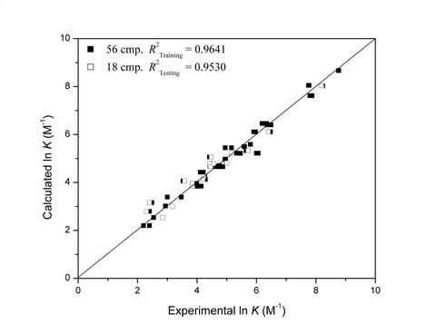
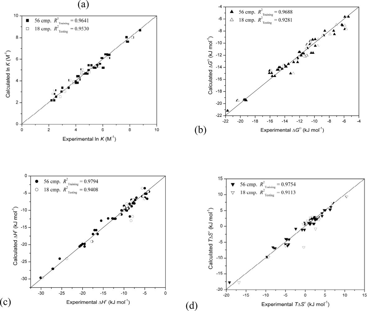
| 4 | 0.9641 | 0.9530 | 12 | 79 | 114 | 134 | |||||
| ΔG° | 8 | 0.9985 | 0.9924 | 3 | 11 | 28 | 79 | 94 | 112 | 136 | 144 |
| 7 | 0.9978 | 0.9928 | 2 | 9 | 111 | 123 | 129 | 133 | 140 | ||
| 6 | 0.9969 | 0.9894 | 3 | 12 | 94 | 124 | 133 | 140 | |||
| 5 | 0.9935 | 0.9849 | 3 | 20 | 27 | 59 | 134 | ||||
| 4 | 0.9688 | 0.9281 | 20 | 72 | 94 | 122 | |||||
| ΔH° | 8 | 0.9987 | 0.9510 | 28 | 54 | 76 | 83 | 124 | 173 | 181 | 186 |
| 7 | 0.9977 | 0.9385 | 20 | 79 | 91 | 140 | 143 | 153 | 187 | ||
| 6 | 0.9965 | 0.9417 | 2 | 21 | 27 | 112 | 154 | 176 | |||
| 5 | 0.9943 | 0.9374 | 16 | 36 | 79 | 91 | 122 | ||||
| 4 | 0.9794 | 0.9408 | 20 | 21 | 30 | 36 | |||||
| TΔS° | 8 | 0.9986 | 0.8949 | 3 | 23 | 36 | 44 | 94 | 112 | 114 | 159 |
| 7 | 0.9982 | 0.9371 | 9 | 20 | 33 | 100 | 122 | 158 | 199 | ||
| 6 | 0.9952 | 0.8991 | 9 | 12 | 93 | 94 | 154 | 164 | |||
| 5 | 0.9868 | 0.9079 | 6 | 30 | 39 | 76 | 90 | ||||
| 4 | 0.9754 | 0.9113 | 8 | 76 | 114 | 129 | |||||
| No. | Class | Description |
|---|---|---|
| 8 | 2D | Weiner polarity number |
| 12 | 2D | PEOE Charge BCUT (3/3) |
| 20 | 2D | Molar Refractivity BCUT (3/3) |
| 21 | 2D | PEOE Charge GCUT (0/3) |
| 30 | 2D | Molar Refractivity GCUT (1/3) |
| 36 | 2D | Atom information content (mean) |
| 50 | 2D | Number of chiral centers |
| 72 | 2D | Total positive partial charge |
| 76 | 2D | Total positive 0 van der Waals surface area |
| 79 | 2D | Total positive 3 van der Waals surface area |
| 94 | 2D | Fractional positive van der Waals surface area |
| 114 | 2D | Third alpha modified shape index |
| 122 | 2D | Number of H-bond donor atoms |
| 129 | 2D | van der Waals polar surface area |
| 134 | 2D | Bin 3 SlogP_(0.00, 0.10] |
© 2009 by the authors; licensee Molecular Diversity Preservation International, Basel, Switzerland. This article is an open-access article distributed under the terms and conditions of the Creative Commons Attribution license (http://creativecommons.org/licenses/by/3.0/).
Share and Cite
Prakasvudhisarn, C.; Wolschann, P.; Lawtrakul, L. Predicting Complexation Thermodynamic Parameters of β-Cyclodextrin with Chiral Guests by Using Swarm Intelligence and Support Vector Machines. Int. J. Mol. Sci. 2009, 10, 2107-2121. https://doi.org/10.3390/ijms10052107
Prakasvudhisarn C, Wolschann P, Lawtrakul L. Predicting Complexation Thermodynamic Parameters of β-Cyclodextrin with Chiral Guests by Using Swarm Intelligence and Support Vector Machines. International Journal of Molecular Sciences. 2009; 10(5):2107-2121. https://doi.org/10.3390/ijms10052107
Chicago/Turabian StylePrakasvudhisarn, Chakguy, Peter Wolschann, and Luckhana Lawtrakul. 2009. "Predicting Complexation Thermodynamic Parameters of β-Cyclodextrin with Chiral Guests by Using Swarm Intelligence and Support Vector Machines" International Journal of Molecular Sciences 10, no. 5: 2107-2121. https://doi.org/10.3390/ijms10052107