Density Functional Studies of Molecular Polarizabilities. 10. Fulvenes and Fulvalenes

Abstract

We report accurate Ab Initio Hartree Fock (HF) and Density Functional Theory (DFT) studies of the static dipole polarizabilities and first hyperpolarizabilities of the [n] fulvene and the [n,m] fulvalene series of molecules (with n, m = 3,5,7). Calculations are also reported for the parent cycloalkenes: cyclopropene, cyclopentadiene and cycloheptatriene (1-3 respectively). Geometries were optimized at the HF/6-311G(3d,2p) level of theory. All the fulvenes (4-6) and the smaller fulvalenes (7, 9 and 10) are found to be planar. Pentaheptafulvalene (11) is slightly non-planar whilst heptafulvalene (12) has a folded C_2h structure. Calculated C-C bond lengths are consistently smaller than the experimental values. Dipole polarizabilities and non-zero hyperpolarizabilities were calculated at the HF/6-311++G(3d,2p) and BLYP/6-311++G(3d,2p) levels of theory, using HF/6-311G(3d,2p) geometries. Dipole polarizabilities correlate well with those given on the basis of atom additivity. Molecules (8), (9) and (11) show very large dipole hyperpolarizabilities.

Introduction

The monocyclic (poly)enes cyclopropene (1), cyclopentadiene (2) and cycloheptatriene (3) may be regarded as building blocks from which both the fulvene and fulvalene families of molecules can be constructed [1].

The fulvenes triafulvene (4), pentafulvene (5) and heptafulvene (6) have attracted much interest due to their cross-conjugated structures and questions regarding their aromatic/ antiaromatic character.

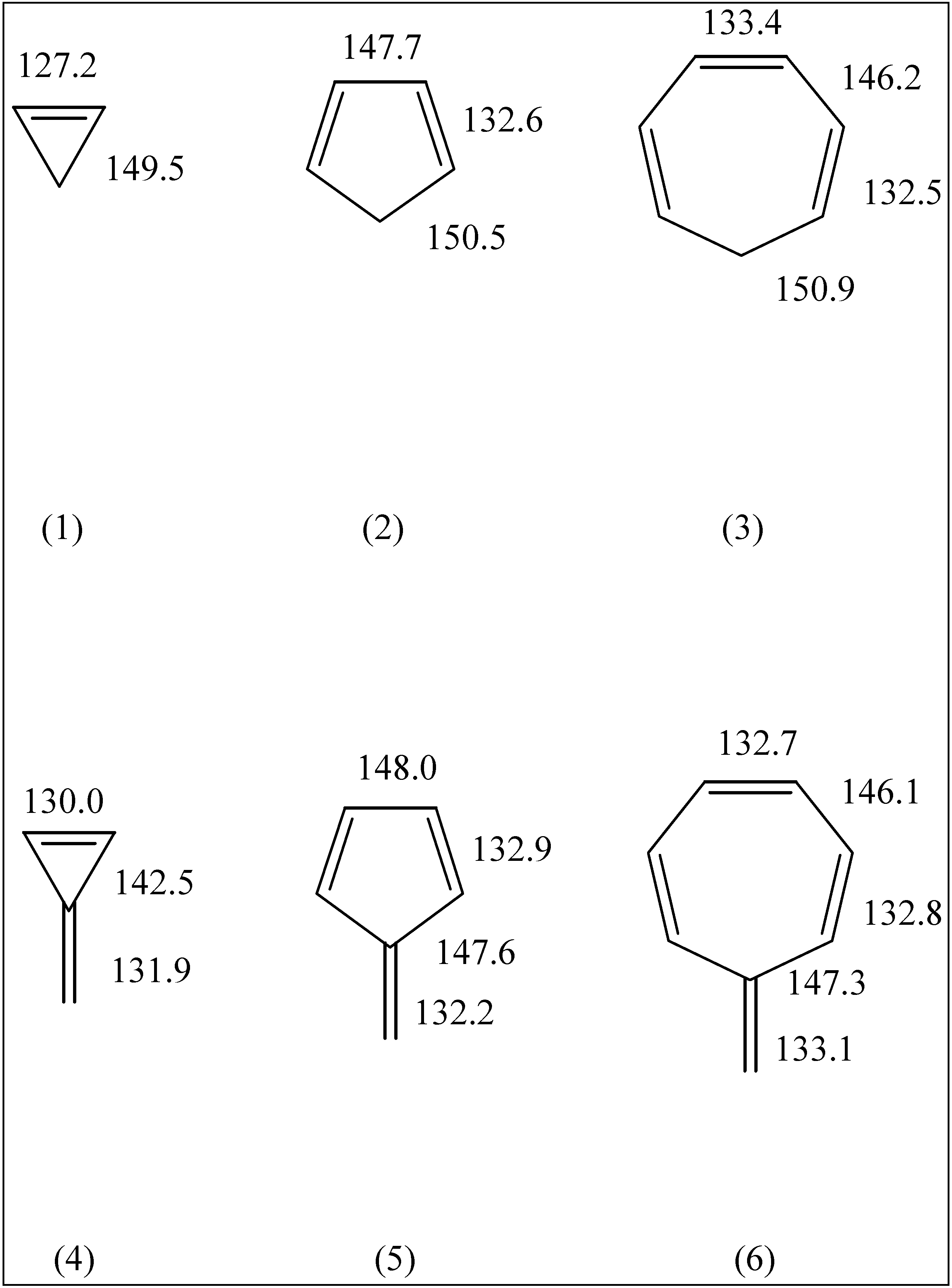
Figure 1. HF geometries of molecules 1 through 6.

Figure 1. HF geometries of molecules 1 through 6.

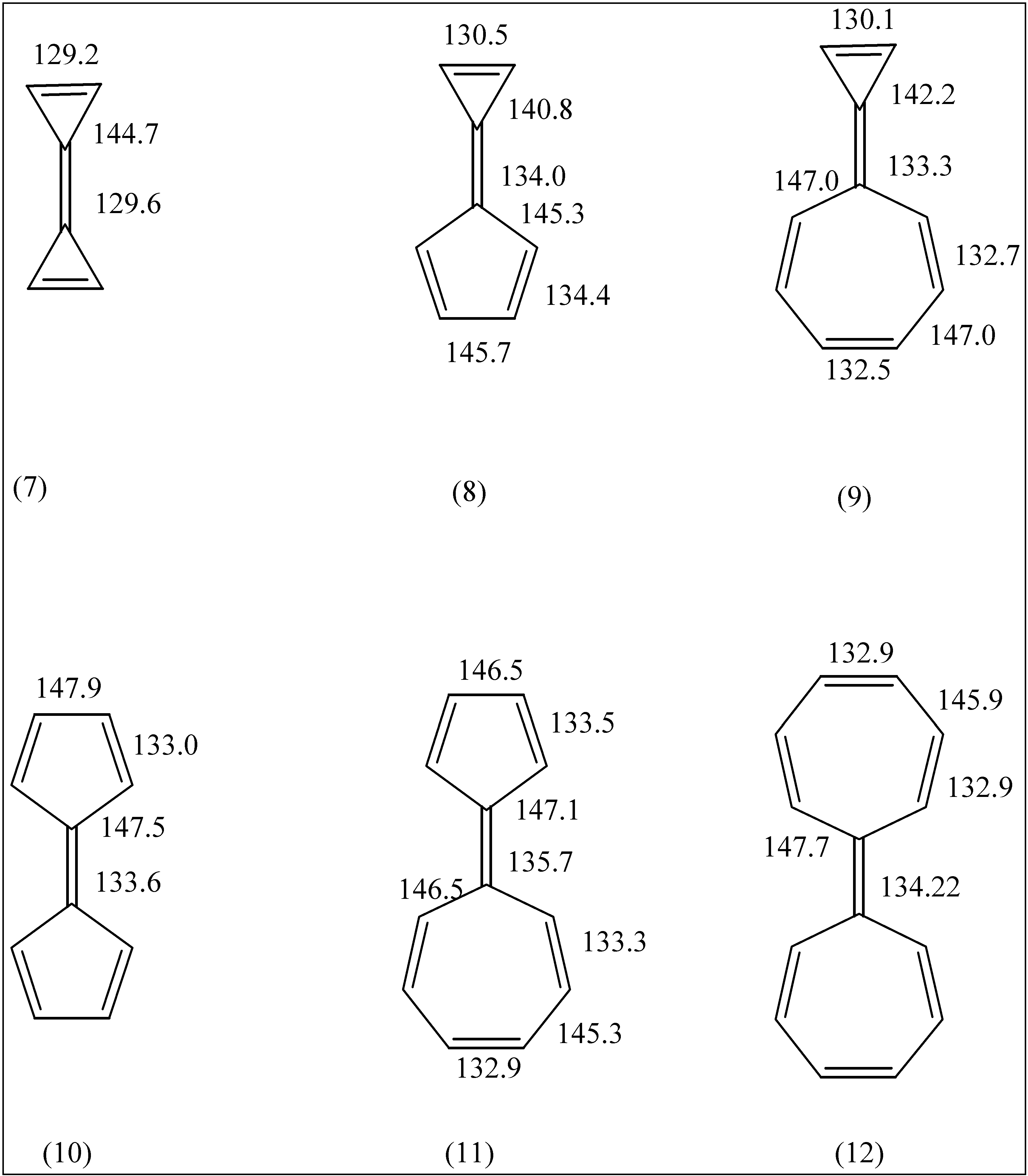
The fulvalenes triafulvalene (7), triapentafulvalene (8), triaheptafulvalene (9) and pentafulvalene (10) have also received a great deal of attention in the literature. The small fulvalenes (7-9) have not been synthesized, but a great deal is known about the chemistry of 12; it is non-planar with a marked alternation of long and short bonds in the seven membered rings and it has a relatively long central C=C bond.

Figure 2. HF geometries of molecules 7 through 12.

Figure 2. HF geometries of molecules 7 through 12.

The electric moments of a molecule are quantities of fundamental importance in structural chemistry. When a molecule with permanent electric dipole moment p_e is subject to an external constant electrostatic field E, the change in the dipole moment can be written in tensor notation as [2]

p_e(E) = p_e(0) + α:E + ½ β:EE+...

(1)

Here p_e(0) is the dipole in the absence of a field and p_e(E) is the dipole moment in the presence of the field. The six independent quantities α_ij ( j ≥ i) define the dipole polarizability tensor, the ten independent quantities β_ijk define the first dipole hyperpolarizability and so on.

Hyperpolarizabilities are important when the applied electric field is large. There has recently been an intense search for molecules with large non-zero hyperpolarizabilities [3], since these substances have potential as the constituents of non-linear optical materials.

The energy U of the molecular charge distribution also changes when an electrostatic field is applied. This change can be written as

U (E) = U (0) − p_e(0).E − ½ α:EE − 1/6 β:EEE−....

(2)

Equations (1) and (2) are the key equations for the calculation of molecular polarizabilities and hyperpolarizabilities by gradient techniques [3]. The dipole polarizability is obtained as the first derivative of the induced dipole with respect to the applied field or the second derivative of the energy. The dipole hyperpolarizability is obtained as the second derivative of the induced dipole with respect to the applied field, and so on. Analytical gradient expressions are available at many levels of theory, otherwise they have to be found by numerical techniques.

The experimental determination of a molecular polarizability is far from straightforward, especially if the molecule has little or no symmetry. For a molecule with symmetry, the principal axes of the polarizability tensor correspond to the symmetry axes. Otherwise the principal axes have to be determined by diagonalization of the polarizability matrix. The principal axes are usually referred to as ‘a’, ‘b’ and ‘c’. We will adopt the convention

α_aa < α_bb < α_cc

(3)

where the α_ii are the eigenvalues of the polarizability matrix.

The mean value

< α >=1/3(α_aa + α_bb + α_cc)

(4)

can be determined from the refractive index n of a gas according to the equation

$$n=1+\frac{<\alpha >p}{2{\in }_0{k}_{B}T}$$

(5)

where p is the pressure, kB the Boltzmann constant, T the thermodynamic temperature and ꇊ₀ the permittivity of free space. A key assumption in the derivation of equation (5) is that the individual molecules are sufficiently far apart on average that they do not interact with each other.

In a condensed phase, the problem is more complicated because the separation between molecules is of the order of molecular dimensions and their interactions can no longer be ignored. As a result both the external field and the field due to the surrounding molecules polarize each molecule.

The Lorenz-Lorentz equation

$$\frac{n^2-1}{n^2+2}=\frac{N<\alpha >}{3{\in }_{0}V}$$

(6)

applies to non-polar molecules in condensed phases and it can be derived from a detailed consideration of these ideas [1]. Here, N is the number of molecules in volume V. Rewriting equation (6) in terms of molar quantities defines the molar refractivity

$$R_M=\frac{M}{\rho }\frac{n^2-1}{n^2+2}=\frac{N_A<\alpha >}{3{\in }_{0}V}$$

(7)

Here M is the molar mass, N_A the Avogadro constant and ρ the density. It appears to be an experimental fact that molar refractivities are additive properties at the molecular level, and a view has long prevailed that the molar refractivity of a molecule is a sum of the molar refractivities of the constituent parts (atoms/ groups) [5]. Extensive tables of additive atom and group molar refractivities are available [5,6]. These tables have been extended to molecular polarizabilities with the compilations of Denbigh [6] and others.

In the case of molecules with a permanent dipole moment, it is necessary to take account of the orientation polarization. The Debye equation

$$\frac{M}{\rho }\frac{{\in }_r-1}{{\in }_r+2}=\frac{N_A}{3{\in }_0}\left(<\alpha >+\frac{p_e^2}{3k_{B}T}\right)$$

(8)

permits polarizabilities and dipole moments to be determined from measurements of the relative permittivity ∈_r and the density ρ as a function of temperature. Reliable results can only be obtained from dilute solutions [1].

There is a large literature concerning semi-empirical calculations of dipole polarizabilities and hyperpolarizabilities of organic molecules. It is usually found that the in-plane components of α are well represented at (for example) the AM1 level of theory, but that the perpendicular component is very much smaller than the experimental value.

A few authors have used Ab Initio techniques to study molecular polarizabilities. It is common knowledge that polarizabilities can only be calculated accurately by employing extended basis sets. In particular, these basis sets have to include diffuse functions that can accurately describe the response of a molecular charge distribution to an external electric field. Such diffuse (s and p) functions are needed in addition to the normal polarization functions; they are denoted by + and ++ in packages such as GAUSSIAN98 [7].

Once near the Hartree Fock limit, it is necessary to concern oneself with the correlation contribution to such properties. In recent years, density functional techniques have received a great deal of attention in the literature. In Density functional theory (DFT) we write the electronic energy expression [4,8] as

ε_el = Tr(h₁P) + ½ Tr(PJ) + ε_X + ε_C

(9)

where ε_X is the exchange functional and ε_C the correlation functional. In order to calculate ε_X and ε_C it is necessary to give some functional form to the two potentials and then calculate the contribution to the electronic energy as an integral over the electron density (and occasionally the gradient of the electron density). These calculations are performed numerically. There are many variants on the form of the exchange and the correlation functional, most of which are based on the free-electron gas model [4,8].

In two earlier notes in this Series [9,10], we reported polarizability studies for pentafulvene (5) and pentafulvalene (10). The aim of this paper is to collect results for the full series of molecules 1-12.

Calculations

A. Geometries and dipole moments

All Ab Initio calculations were made using Gaussian98 [7]. Geometries were optimized at the HF/6-311G(3d,2p) level of theory.

For the record, the Ab Initio total energies and electric dipole moments are given in Table 1.

Table 1. Total energies ε and dipole moments pe for molecules 1-12.

Molecule	Key	- ε / Eh*	pe / D*
cyclopropene	1	115.858663	0.5267
cyclopentadiene	2	192.847328	0.3399
cycloheptatriene	3	269.757718	0.3343
triafulvene	4	153.715377	2.3963
pentafulvene	5	230.709509	0.4060
heptafulvene	6	307.621691	0.4039
triafulvalene	7	229.345393	0
triapentafulvalene	8	306.374585	4.9764
triaheptafulvalene	9	383.274605	3.7578
pentafulvalene	10	383.359632	0
Pentaheptafulvalene	11	460.270703	2.2248
heptafulvalene	12	537.177307	0

*Conversion factors to SI are as follows; 1 hartree, E_h ≅ 4.3598 × 10^-18 J 1 debye, D ≅ 3.336 × 10^-30 C m.

Table 1. Total energies ε and dipole moments pe for molecules 1-12.

Molecule	Key	- ε / Eh*	pe / D*
cyclopropene	1	115.858663	0.5267
cyclopentadiene	2	192.847328	0.3399
cycloheptatriene	3	269.757718	0.3343
triafulvene	4	153.715377	2.3963
pentafulvene	5	230.709509	0.4060
heptafulvene	6	307.621691	0.4039
triafulvalene	7	229.345393	0
triapentafulvalene	8	306.374585	4.9764
triaheptafulvalene	9	383.274605	3.7578
pentafulvalene	10	383.359632	0
Pentaheptafulvalene	11	460.270703	2.2248
heptafulvalene	12	537.177307	0

*Conversion factors to SI are as follows; 1 hartree, E_h ≅ 4.3598 × 10^-18 J 1 debye, D ≅ 3.336 × 10^-30 C m.

A full study of the geometries and electric dipole moments of these molecules at the HF/6-31G* and MP2/6-31G* levels of theory has been given by Scott et. al. [1]. Since our HF results are very similar to theirs, we simply note the salient C-C bond lengths in Figure 1 and Figure 2. All the fulvenes (4-6) and the smaller fulvalenes (7, 9 and 10) are found to be planar. Pentaheptafulvalene (11) is slightly non-planar whilst heptafulvalene (12) has a folded C_2h structure. The calculated C-C bond lengths are consistently smaller than the experimental values. Such behaviour is common for HF calculations on molecules with multiple bonds.

B. Polarizabilities

Polarizabilities were calculated at the HF/6-311G(3d,2p) // HF/6-311++G(3d,2p) and HF/6311G(3d,2p) // BLYP/6-311++G(3d,2p) levels of theory. That is, the geometries discussed above were used unchanged, but two sets of extra diffuse s and p functions were added to the basis sets for the purpose of polarizability calculations.

Dipole polarizabilities calculated at the HF level of theory are shown in Table 2.

Table 2. Principal dipole polarizability tensor components (HF).

Molecule	αaa / au*	αbb	αcc	<α>
1	26.863	35.555	36.031	32.816
2	41.076	58.844	64.517	54.812
3	57.287	86.666	92.616	78.856
4	32.943	41.913	65.566	46.807
5	45.628	65.052	104.717	71.799
6	57.889	95.501	146.247	99.879
7	42.299	62.725	104.999	70.008
8	56.058	85.029	151.931	97.673
9	67.858	113.537	193.133	124.843
10	67.812	101.817	213.058	127.562
11	80.122	132.732	285.781	166.212
12	101.169	159.462	287.267	182.633

* Atomic unit of polarizability e² a₀² E_h^-1 ≈ 1.649 × 10^-41C² m² J^-1, equivalent to 1.4818 × 10^-25 cm³.

Table 2. Principal dipole polarizability tensor components (HF).

Molecule	αaa / au*	αbb	αcc	<α>
1	26.863	35.555	36.031	32.816
2	41.076	58.844	64.517	54.812
3	57.287	86.666	92.616	78.856
4	32.943	41.913	65.566	46.807
5	45.628	65.052	104.717	71.799
6	57.889	95.501	146.247	99.879
7	42.299	62.725	104.999	70.008
8	56.058	85.029	151.931	97.673
9	67.858	113.537	193.133	124.843
10	67.812	101.817	213.058	127.562
11	80.122	132.732	285.781	166.212
12	101.169	159.462	287.267	182.633

* Atomic unit of polarizability e² a₀² E_h^-1 ≈ 1.649 × 10^-41C² m² J^-1, equivalent to 1.4818 × 10^-25 cm³.

The corresponding results at BLYP level are shown in Table 3.

Table 3. Principal dipole polarizability tensor components (BLYP).

Molecule	αaa / au	αbb	αcc	<α>
1	28.153	36.908	38.820	34.627
2	42.523	64.667	67.458	58.216
3	60.273	94.617	98.119	84.336
4	33.809	44.115	67.630	48.518
5	46.266	71.108	103.363	73.579
6	58.484	103.872	149.783	104.046
7	43.342	65.394	110.142	72.959
8	56.904	91.458	154.105	100.822
9	68.827	122.486	202.319	131.211
10	68.581	111.201	211.555	130.446
11	80.706	144.867	291.086	172.22
12	104.681	174.461	311.392	196.845

Table 3. Principal dipole polarizability tensor components (BLYP).

Molecule	αaa / au	αbb	αcc	<α>
1	28.153	36.908	38.820	34.627
2	42.523	64.667	67.458	58.216
3	60.273	94.617	98.119	84.336
4	33.809	44.115	67.630	48.518
5	46.266	71.108	103.363	73.579
6	58.484	103.872	149.783	104.046
7	43.342	65.394	110.142	72.959
8	56.904	91.458	154.105	100.822
9	68.827	122.486	202.319	131.211
10	68.581	111.201	211.555	130.446
11	80.706	144.867	291.086	172.22
12	104.681	174.461	311.392	196.845

The BLYP polarizabilities are generally a few percent higher than the corresponding values calculated at HF level.

We discussed above the possibility that molecular polarizabilities could be decomposed into contributions from the constituent atoms and/ or groups. In an earlier paper [11], we suggested the following atom contributions (Table 4) based on our analysis of a number of conjugated hydrocarbons.

Table 4. Atom Contributions to <α>.

Level of theory	αC / au.	αH/ au
HF/6-311++G(3d,2p)	8.3020	2.3606
BLYP/6-311++G(3d,2p)	7.9110	3.3772

Table 4. Atom Contributions to <α>.

Level of theory	αC / au.	αH/ au
HF/6-311++G(3d,2p)	8.3020	2.3606
BLYP/6-311++G(3d,2p)	7.9110	3.3772

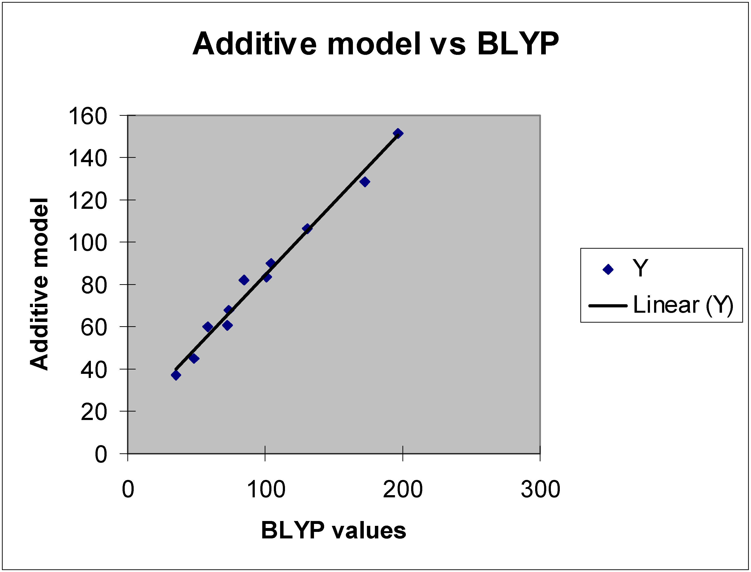
These values can be used to calculate the mean polarizabilities for molecules 1 through 12. Analysis shows a good straight-line relationship, but poor overall absolute agreement between the BLYP values and those predicted on the basis of simple additivity. Re-analysis of the atom polarizability values needed to give good absolute agreement with experiment along the lines discussed in [11] suggests that the BLYP values in Table 4 should be adjusted to 15.68 and –2.75 au.

Figure 3. Regression analysis.

Figure 3. Regression analysis.

The “additive group” model has been criticised on the grounds that it does not allow for the interaction between atoms and groups in a molecule [12]. Nevertheless, it can sometimes give useful chemical insight. Thus the BLYP results for ethane, ethene and cyclopropane are given in Table 5, for comparison against cyclopropene (1).

Table 5. BLYP mean polarizabilities.

Molecule	<α> / au
Ethane	29.007
Ethene	27.454
Cyclopropane	36.900
Cyclopropene (1)	34.627

Table 5. BLYP mean polarizabilities.

Molecule	<α> / au
Ethane	29.007
Ethene	27.454
Cyclopropane	36.900
Cyclopropene (1)	34.627

Cyclopropene has a smaller <α> than cyclopropane. If we regard cyclopropene as ethene plus a carbon atom, then the additive model gives an <α> of 35.365, in modest agreement with the full BLYP calculation. Likewise, ethane plus a carbon atom gives a predicted <α> = 36.918 au for cyclopropane, again in modest agreement with the calculated value.

Cyclopentane has <α> = 63.592 au, which is to be compared with a value for cyclopentadiene (2) plus two hydrogen atoms of 64.970 au.

The Ab Initio dipole polarizabilities for 9 and 10 are almost identical.

There is no experimental data in the literature.

C. Hyperpolarizabilities

Hyperpolarizability data is also hard to come by, both experimentally and theoretically. There is no experimental data in the literature for any of the molecules 1 through 12. The tensor components for molecules 1 through 6 are shown in Table 6, and those for the remaining molecules in Table 7.

Table 6. Hyperpolarizability tensor components (HF/6-311++G(3d,2p)) for (1) through (6)*.

Component	1	2	3	4	5	6
aaa	0	0	-13.99	.02	0	.02
aab	.01	0	0	0	0	0
aac	-10.02	10.73	-4.78	61.38	-4.85	25.70
abb	0	-.02	17.99	.01	0	0
abc	0	0	0	0	0	0
acc	0	.01	-8.92	.04	0	-.04
bbb	.12	0	0	0	0	0
bbc	-57.80	-16.63	6.56	-59.05	-26.26	-3.66
bcc	-.10	0	0	0	0	0
ccc	19.87	35.05	0.91	-10.24	-2.76	210.14

The atomic unit of β is E_h^-2a₀²e², approximately 3.206 × 10^-53 C³ m³ J^-2.

Table 6. Hyperpolarizability tensor components (HF/6-311++G(3d,2p)) for (1) through (6)*.

Component	1	2	3	4	5	6
aaa	0	0	-13.99	.02	0	.02
aab	.01	0	0	0	0	0
aac	-10.02	10.73	-4.78	61.38	-4.85	25.70
abb	0	-.02	17.99	.01	0	0
abc	0	0	0	0	0	0
acc	0	.01	-8.92	.04	0	-.04
bbb	.12	0	0	0	0	0
bbc	-57.80	-16.63	6.56	-59.05	-26.26	-3.66
bcc	-.10	0	0	0	0	0
ccc	19.87	35.05	0.91	-10.24	-2.76	210.14

The atomic unit of β is E_h^-2a₀²e², approximately 3.206 × 10^-53 C³ m³ J^-2.

Table 7. Hyperpolarizability tensor components (HF/6-311++G(3d,2p)) for (7) through (12).

Component	7	8	9	10	11	12
aaa	0	0	-.016	0	-.026	0
aab	0	0	-.730	0	.339	0
aac	0	63.617	24.409	0	45.080	0
abb	0	.168	-.013	0	.146	0
abc	0	.003	0	0	.015	0
acc	0	-.189	.015	0	-.157	0
bbb	0	-.002	0	0	.220	0
bbc	0	6.606	30.038	0	140.918	0
bcc	0	.002	.008	0	-.187	0
ccc	0	-329.424	676.918	0	732.070	0

Table 7. Hyperpolarizability tensor components (HF/6-311++G(3d,2p)) for (7) through (12).

Component	7	8	9	10	11	12
aaa	0	0	-.016	0	-.026	0
aab	0	0	-.730	0	.339	0
aac	0	63.617	24.409	0	45.080	0
abb	0	.168	-.013	0	.146	0
abc	0	.003	0	0	.015	0
acc	0	-.189	.015	0	-.157	0
bbb	0	-.002	0	0	.220	0
bbc	0	6.606	30.038	0	140.918	0
bcc	0	.002	.008	0	-.187	0
ccc	0	-329.424	676.918	0	732.070	0

Molecules (7), (10) and (12) have zero dipole hyperpolarizabilities, on account of their geometries. The dipole hyperpolarizabilities of a conjugated molecule can be greatly enhanced by the presence of a donor and acceptor group located at either end of the conjugation path. Strong donors and acceptors exert the largest effect [13], and the nature of the conjugation path between the donor and acceptor group is also of great importance. It is interesting to note the large dipole hyperpolarizabilities of molecules 8, 9 and 11, which is consistent with this charge transfer mechanism.

All our calculations refer to static fields. The interaction of molecules with oscillating electric fields leads to different non-linear optical processes typified by the electro-optic Pockels effect (EOPE), second harmonic generation (SHG), optical rectification (OR), DC-electric field induced (EFI)SHG, third harmonic generation (THG), Optical Kerr Effect (OKE), DC-electric field induced (FEI)OR etc. These optical processes have to be handled theoretically using so-called time dependent techniques.