
All-Atom Molecular Dynamics of Pure Water–Methane Gas Hydrate Systems under Pre-Nucleation Conditions: A Direct Comparison between Experiments and Simulations of Transport Properties for the Tip4p/Ice Water Model


Abstract
:1. Introduction
2. Material and Methods
2.1. Software Packages
2.2. Simulation Design
2.2.1. Force Field
2.2.2. LAMMPS Input
2.2.3. Methane Systems
2.3. Equilibration Procedure
2.4. Replicate Production Runs
2.5. Transport Property Calculations
3. Results and Discussion
3.1. Molecular Simulation Design Considerations
3.1.1. Consecutive Equilibration Steps
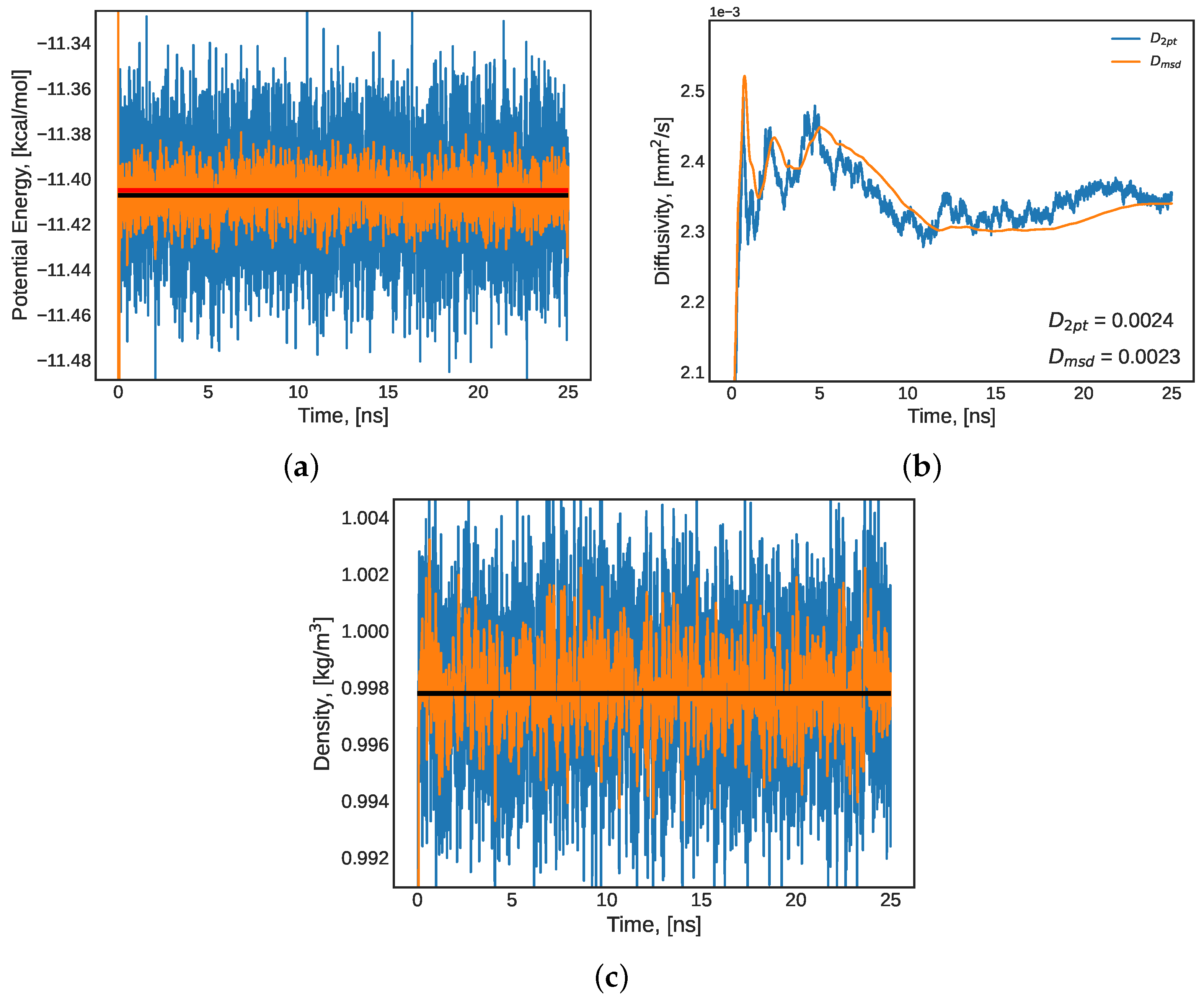
3.1.2. Long-Term Equilibrium Indicators
3.1.3. Hydrogen Bonding Effects
3.2. Water Models
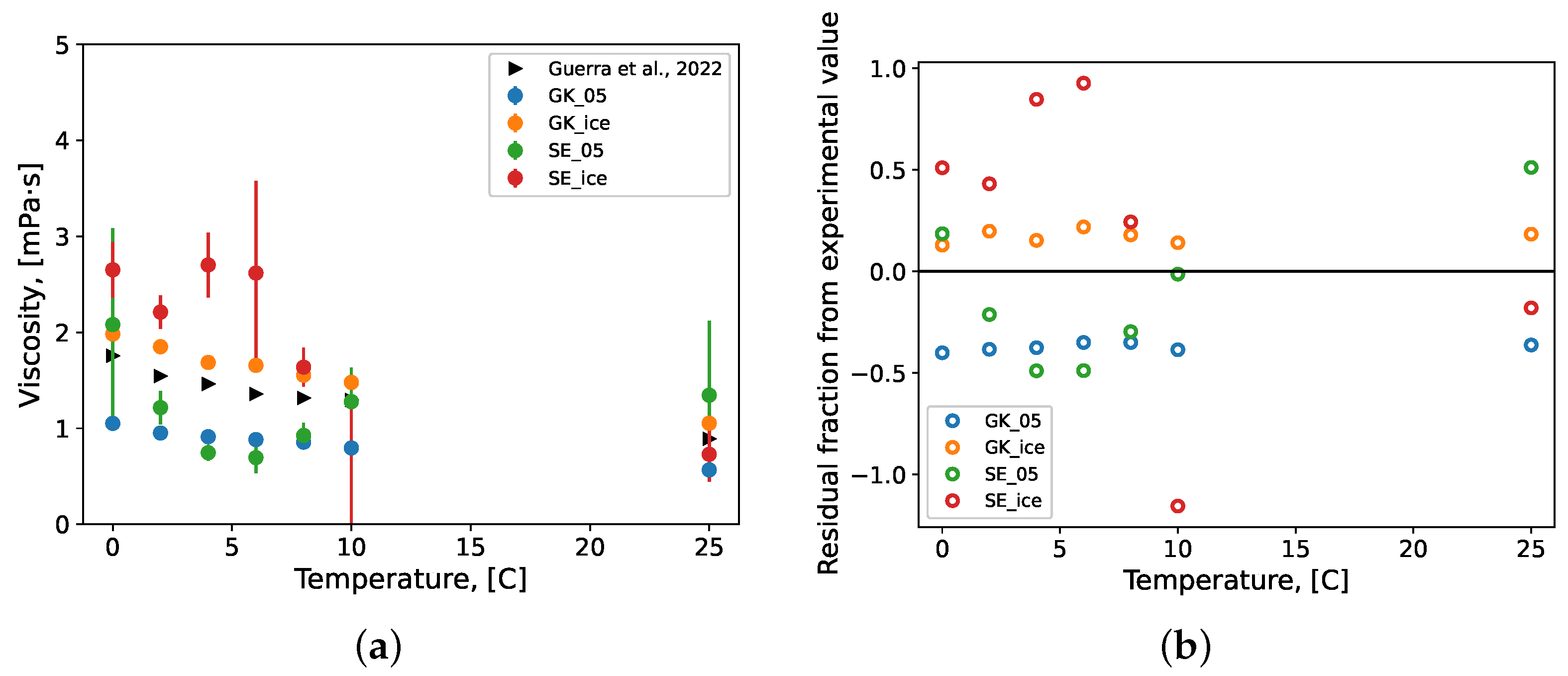
3.2.1. Viscosity
3.2.2. Diffusivity and Thermal Conductivity
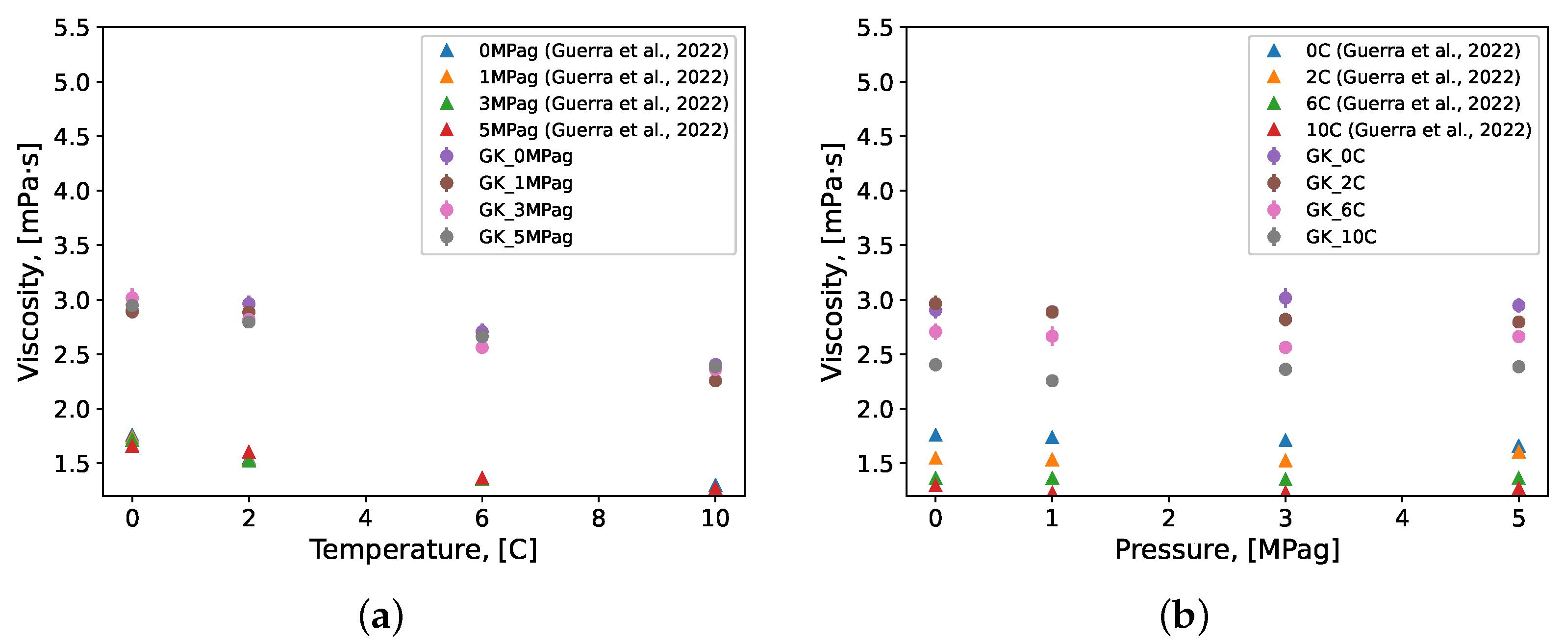
3.3. Methane Gas Hydrate Systems
3.4. Hydrogen Bond Analyses
4. Conclusions and Future Work
Author Contributions
Funding
Institutional Review Board Statement
Informed Consent Statement
Data Availability Statement
Acknowledgments
Conflicts of Interest
Sample Availability
Abbreviations
| AA | All-atom |
| DFT | Density functional theory |
| Eins | Einstein |
| EOS | Equation of state |
| GK | Green–Kubo |
| H-bond | Hydrogen bond |
| LAMMPS | Large-scale Atomic/Molecular Massively Parallel Simulator |
| LJ | Lennard-Jones |
| MD | Molecular dynamics |
| MSD | Mean squared displacement |
| NPT | Isothermal-isobaric ensemble |
| NVT | Canonical ensemble |
| OPLS | Optimized potentials for liquid simulations |
| OPLS-AA | Optimized potentials for liquid simulations all-atom |
| OPLS-UA | Optimized potentials for liquid simulations united-atom |
| Probability distribution function | |
| RMSD | Root mean squared displacement |
| SE | Stokes–Einstein |
| TIP4P | Transferable intermolecular potential with 4 points |
| UA | United atom |
| VACF | Velocity autocorrelation function |
References
- Sloan, E.; Koh, C. Clathrate Hydrates of Natural Gases, 3rd ed.; Taylor and Francis: Boca Raton, FL, USA, 2008. [Google Scholar]
- Carroll, J. Natural Gas Hydrates: A Guide for Engineers, 3rd ed.; Gulf Professional Publishing: Calgary, AB, Canada, 2014. [Google Scholar]
- Sloan, E.; Koh, C.; Sum, A.K. Natural Gas Hydrates in Flow Assurance; Gulf Professional Publishing: Houston, TX, USA, 2011. [Google Scholar]
- Hammerschmidt, E. Formation of gas hydrates in natural gas transmission lines. Ind. Eng. Chem. 1934, 26, 851–855. [Google Scholar] [CrossRef]
- Posteraro, D.; Verrett, J.; Maric, M.; Servio, P. New insights into the effect of polyvinylpyrrolidone (PVP) concentration on methane hydrate growth. 1. Growth rate. Chem. Eng. Sci. 2015, 126, 99–105. [Google Scholar] [CrossRef]
- Posteraro, D.; Ivall, J.; Maric, M.; Servio, P. New insights into the effect of polyvinylpyrrolidone (PVP) concentration on methane hydrate growth. 2. Liquid phase methane mole fraction. Chem. Eng. Sci. 2015, 126, 91–98. [Google Scholar] [CrossRef]
- Heidaryan, E.; Salarabadi, A.; Moghadasi, J.; Dourbash, A. A new high performance gas hydrate inhibitor. J. Nat. Gas Chem. 2010, 19, 323–326. [Google Scholar] [CrossRef]
- Daraboina, N.; Pachitsas, S.; Von Solms, N. Natural gas hydrate formation and inhibition in gas/crude oil/aqueous systems. Fuel 2015, 148, 186–190. [Google Scholar] [CrossRef]
- Zhukov, A.Y.; Stolov, M.A.; Varfolomeev, M.A. Use of Kinetic Inhibitors of Gas Hydrate Formation in Oil and Gas Production Processes: Current State and Prospects of Development. Chem. Technol. Fuels Oils 2017, 53, 377–381. [Google Scholar] [CrossRef]
- Rajput, F.; Colantuoni, A.; Bayahya, S.; Dhane, R.; Servio, P.; Maric, M. Poly(styrene/pentafluorostyrene)-block-poly(vinyl alcohol/vinylpyrrolidone) amphiphilic block copolymers for kinetic gas hydrate inhibitors: Synthesis, micellization behavior, and methane hydrate kinetic inhibition. J. Polym. Sci. Part Polym. Chem. 2018, 56, 2445–2457. [Google Scholar] [CrossRef]
- Rajput, F.; Maric, M.; Servio, P. Amphiphilic Block Copolymers with Vinyl Caprolactam as Kinetic Gas Hydrate Inhibitors. Energies 2021, 14, 341. [Google Scholar] [CrossRef]
- Webb, E.B.; Rensing, P.J.; Koh, C.A.; Sloan, E.D.; Sum, A.K.; Liberatore, M.W. High-Pressure Rheology of Hydrate Slurries Formed from Water-in-Oil Emulsions. Energy Fuels 2012, 26, 3504–3509. [Google Scholar] [CrossRef]
- Webb, E.B.; Koh, C.A.; Liberatore, M.W. Rheological Properties of Methane Hydrate Slurries Formed From AOT + Water + Oil Microemulsions. Langmuir 2013, 29, 10997–11004. [Google Scholar] [CrossRef]
- Webb, B.E.; Koh, A.C.; Liberatore, W.M. High Pressure Rheology of Hydrate Slurries Formed from Water-in-Mineral Oil Emulsions. Ind. Eng. Chem. Res. 2014, 53, 6998–7007. [Google Scholar] [CrossRef]
- Sun, B.; Fu, W.; Wang, Z.; Xu, J.; Chen, L.; Wang, J.; Zhang, J. Characterizing the Rheology of Methane Hydrate Slurry in a Horizontal Water-Continuous System. SPE J. 2020, 25, 1026–1041. [Google Scholar] [CrossRef]
- Pandey, G.; Linga, P.; Sangwai, J.S. High pressure rheology of gas hydrate formed from multiphase systems using modified Couette rheometer. Rev. Sci. Instrum. 2017, 88, 25102. [Google Scholar] [CrossRef]
- Pandey, G.; Sangwai, J.S. High pressure rheological studies of methane hydrate slurries formed from water-hexane, water-heptane, and water-decane multiphase systems. J. Nat. Gas Sci. Eng. 2020, 81, 103365. [Google Scholar] [CrossRef]
- Majid, A.A.A.; Wu, D.T.; Koh, C.A. A Perspective on Rheological Studies of Gas Hydrate Slurry Properties. Engineering 2018, 4, 321–329. [Google Scholar] [CrossRef]
- Eslamimanesh, A.; Mohammadi, A.H.; Richon, D.; Naidoo, P.; Ramjugernath, D. Application of gas hydrate formation in separation processes: A review of experimental studies. J. Chem. Thermodyn. 2012, 46, 62–71. [Google Scholar] [CrossRef]
- Fan, S.; Li, S.; Wang, J.; Lang, X.; Wang, Y. Efficient capture of CO2 from simulated flue gas by formation of TBAB or TBAF semiclathrate hydrates. Energy Fuels 2009, 23, 4202–4208. [Google Scholar] [CrossRef]
- Aaron, D.; Tsouris, C. Separation of CO2 from Flue Gas: A Review. Sep. Sci. Technol. 2005, 40, 321–348. [Google Scholar] [CrossRef]
- Linga, P.; Adeyemo, A.; Englezos, P. Medium-Pressure Clathrate Hydrate/Membrane Hybrid Process for Postcombustion Capture of Carbon Dioxide. Environ. Sci. Technol. 2007, 42, 315–320. [Google Scholar] [CrossRef]
- Kang, S.P.; Lee, H. Recovery of CO2 from flue gas using gas hydrate: Thermodynamic verification through phase equilibrium measurements. Environ. Sci. Technol. 2000, 34, 4397–4400. [Google Scholar] [CrossRef]
- Gudmundsson, J.; Parlaktuna, M.; Khokhar, A. Storage of natural gas as frozen hydrate. SPE Prod. Facil. 1994, 9, 69–73. [Google Scholar] [CrossRef]
- Mimachi, H.; Takahashi, M.; Takeya, S.; Gotoh, Y.; Yoneyama, A.; Hyodo, K.; Takeda, T.; Murayama, T. Effect of Long-Term Storage and Thermal History on the Gas Content of Natural Gas Hydrate Pellets under Ambient Pressure. Energy Fuels 2015, 29, 4827–4834. [Google Scholar] [CrossRef]
- Park, K.N.; Hong, S.Y.; Lee, J.W.; Kang, K.C.; Lee, Y.C.; Ha, M.G.; Lee, J.D. A new apparatus for seawater desalination by gas hydrate process and removal characteristics of dissolved minerals (Na+, Mg2+, Ca2+, K+, B3+). Desalination 2011, 274, 91–96. [Google Scholar] [CrossRef]
- McElligott, A.; Uddin, H.; Meunier, J.L.; Servio, P. Effects of Hydrophobic and Hydrophilic Graphene Nanoflakes on Methane Hydrate Kinetics. Energy Fuels 2019, 33, 11705–11711. [Google Scholar] [CrossRef]
- McElligott, A.; Whalen, A.; Du, C.Y.; Näveke, L.; Meunier, J.L.; Servio, P. The behaviour of plasma-functionalized graphene nanoflake nanofluids during phase change from liquid water to solid ice. Nanotechnology 2020, 31, 455703. [Google Scholar] [CrossRef]
- McElligott, A.; Meunier, J.L.; Servio, P. Effects of Hydrophobic and Hydrophilic Graphene Nanoflakes on Methane Dissolution Rates in Water under Vapor–Liquid–Hydrate Equilibrium Conditions. Ind. Eng. Chem. Res. 2021, 60, 2677–2685. [Google Scholar] [CrossRef]
- Guerra, A.; McElligott, A.; Du, Y.C.; Marić, M.; Rey, A.D.; Servio, P. Dynamic viscosity of methane and carbon dioxide hydrate systems from pure water at high-pressure driving forces. Chem. Eng. Sci. 2022, 252, 117282. [Google Scholar] [CrossRef]
- McElligott, A.; Guerra, A.; Du, C.Y.; Rey, A.D.; Meunier, J.L.; Servio, P. Dynamic viscosity of methane hydrate systems from non-Einsteinian, plasma-functionalized carbon nanotube nanofluids. Nanoscale 2022, 28, 702. [Google Scholar] [CrossRef] [PubMed]
- Zhu, X.; Rey, A.D.; Servio, P. Piezo-elasticity and stability limits of monocrystal methane gas hydrates: Atomistic-continuum characterization. Can. J. Chem. Eng. 2022. [Google Scholar] [CrossRef]
- Zhu, X.; Rey, A.D.; Servio, P. Multiscale Piezoelasticity of Methane Gas Hydrates: From Bonds to Cages to Lattices. Energy Fuels 2022. [Google Scholar] [CrossRef]
- Vlasic, T.M.; Servio, P.D.; Rey, A.D. Infrared Spectra of Gas Hydrates from First-Principles. J. Phys. Chem. 2019, 123, 936–947. [Google Scholar] [CrossRef]
- Daghash, S.M.; Servio, P.; Rey, A.D. From Infrared Spectra to Macroscopic Mechanical Properties of sH Gas Hydrates through Atomistic Calculations. Molecules 2020, 25, 5568. [Google Scholar] [CrossRef]
- Mathews, S.L.; Servio, P.D.; Rey, A.D. Heat Capacity, Thermal Expansion Coefficient, and Grüneisen Parameter of CH4, CO2, and C2H6 Hydrates and Ice Ih via Density Functional Theory and Phonon Calculations. Cryst. Growth Des. 2020, 20, 5947–5955. [Google Scholar] [CrossRef]
- Mirzaeifard, S.; Servio, P.; Rey, A.D. Molecular Dynamics Characterization of Temperature and Pressure Effects on the Water-Methane Interface. Colloids Interface Sci. Commun. 2018, 24, 75–81. [Google Scholar] [CrossRef]
- Liu, Y.; Chen, C.; Hu, W.; Li, W.; Dong, B.; Qin, Y. Molecular Dynamics Simulation Studies of Gas Hydrate Growth with Impingement. Chem. Eng. J. 2021, 426, 130705. [Google Scholar] [CrossRef]
- González, M.A.; Abascal, J.L.F. The shear viscosity of rigid water models. J. Chem. Phys. 2010, 132, 96101. [Google Scholar] [CrossRef]
- Montero de Hijes, P.; Sanz, E.; Joly, L.; Valeriani, C.; Caupin, F. Viscosity and self-diffusion of supercooled and stretched water from molecular dynamics simulations. J. Chem. Phys. 2018, 149, 094503. [Google Scholar] [CrossRef]
- Aimoli, C.G.; Maginn, E.J.; Abreu, C.R. Transport properties of carbon dioxide and methane from molecular dynamics simulations. J. Chem. Phys. 2014, 141, 6538. [Google Scholar] [CrossRef]
- Maginn, E.J.; Messerly, R.A.; Carlson, D.J.; Roe, D.R.; Elliot, J.R. Best Practices for Computing Transport Properties 1. Self-Diffusivity and Viscosity from Equilibrium Molecular Dynamics. Living J. Comput. Mol. Sci. 2018, 1, 6324. [Google Scholar] [CrossRef] [Green Version]
- Rapaport, D.C. The Art of Molecular Dynamics Simulation; Cambridge University Press: Cambridge, UK, 2004. [Google Scholar]
- Jiménez-Ángeles, F.; Firoozabadi, A. Nucleation of Methane Hydrates at Moderate Subcooling by Molecular Dynamics Simulations. J. Phys. Chem. C 2014, 118, 11310–11318. [Google Scholar] [CrossRef]
- Liang, S.; Kusalik, P.G. Crystal Growth Simulations of H2S Hydrate. J. Phys. Chem. B 2010, 114, 9563–9571. [Google Scholar] [CrossRef] [PubMed]
- Hawtin, R.W.; Quigley, D.; Rodger, P.M. Gas hydrate nucleation and cage formation at a water/methane interface. Phys. Chem. Chem. Phys. 2008, 10, 4853–4864. [Google Scholar] [CrossRef] [PubMed]
- Moon, C.; Taylor, C.P.; Mark Rodger, P. Molecular Dynamics Study of Gas Hydrate Formation. J. Am. Chem. Soc. 2003, 125, 4706–4707. [Google Scholar] [CrossRef] [PubMed]
- Zhang, J.; Hawtin, W.R.; Yang, Y.; Nakagava, E.; Rivero, M.; Choi, K.S.; Rodger, M.P. Molecular Dynamics Study of Methane Hydrate Formation at a Water/Methane Interface. J. Phys. Chem. B 2008, 112, 10608–10618. [Google Scholar] [CrossRef]
- Walsh, M.R.; Koh, C.A.; Sloan, E.D.; Sum, A.K.; Wu, D.T. Microsecond Simulations of Spontaneous Methane Hydrate Nucleation and Growth. Science 2009, 326, 1095–1098. [Google Scholar] [CrossRef]
- Zhang, Z.; Walsh, M.R.; Guo, G.J. Microcanonical molecular simulations of methane hydrate nucleation and growth: Evidence that direct nucleation to sI hydrate is among the multiple nucleation pathways. Phys. Chem. Chem. Phys. 2015, 17, 8870–8876. [Google Scholar] [CrossRef]
- Guo, G.J.; Mark Rodger, P. Solubility of Aqueous Methane under Metastable Conditions: Implications for Gas Hydrate Nucleation. J. Phys. Chem. B 2013, 117, 6498–6504. [Google Scholar] [CrossRef]
- Yan, L.; Chen, G.; Pang, W.; Liu, J. Experimental and Modeling Study on Hydrate Formation in Wet Activated Carbon. J. Phys. Chem. B 2005, 109, 6025–6030. [Google Scholar] [CrossRef]
- English, N.J.; Johnson, J.K.; Taylor, C.E. Molecular-dynamics simulations of methane hydrate dissociation. J. Chem. Phys. 2005, 123, 244503. [Google Scholar] [CrossRef]
- Baez, L.A.; Clancy, P. Computer Simulation of the Crystal Growth and Dissolution of Natural Gas Hydratesa. Ann. N. Y. Acad. Sci. 1994, 715, 177–186. [Google Scholar] [CrossRef]
- English, N.J.; Clarke, E.T. Molecular dynamics study of CO2 hydrate dissociation: Fluctuation-dissipation and non-equilibrium analysis. J. Chem. Phys. 2013, 139, 94701. [Google Scholar] [CrossRef]
- Ding, L.Y.; Geng, C.Y.; Zhao, Y.H.; Wen, H. Molecular dynamics simulation on the dissociation process of methane hydrates. Mol. Simul. 2007, 33, 1005–1016. [Google Scholar] [CrossRef]
- Myshakin, M.E.; Jiang, H.; Warzinski, P.R.; Jordan, D.K. Molecular Dynamics Simulations of Methane Hydrate Decomposition. J. Phys. Chem. A 2009, 113, 1913–1921. [Google Scholar] [CrossRef]
- Iwai, Y.; Nakamura, H.; Arai, Y.; Shimoyama, Y. Analysis of dissociation process for gas hydrates by molecular dynamics simulation. Mol. Simul. 2010, 36, 246–253. [Google Scholar] [CrossRef]
- Smirnov, G.S.; Stegailov, V.V. Melting and superheating of sI methane hydrate: Molecular dynamics study. J. Chem. Phys. 2012, 136, 44523. [Google Scholar] [CrossRef]
- Geng, C.Y.; Wen, H.; Zhou, H. Molecular Simulation of the Potential of Methane Reoccupation during the Replacement of Methane Hydrate by CO2. J. Phys. Chem. A 2009, 113, 5463–5469. [Google Scholar] [CrossRef]
- Tung, Y.T.; Chen, L.J.; Chen, Y.P.; Lin, S.T. In Situ Methane Recovery and Carbon Dioxide Sequestration in Methane Hydrates: A Molecular Dynamics Simulation Study. J. Phys. Chem. B 2011, 115, 15295–15302. [Google Scholar] [CrossRef]
- Qi, Y.; Ota, M.; Zhang, H. Molecular dynamics simulation of replacement of CH4 in hydrate with CO2. Energy Convers. Manag. 2011, 52, 2682–2687. [Google Scholar] [CrossRef]
- Bai, D.; Zhang, X.; Chen, G.; Wang, W. Replacement mechanism of methane hydrate with carbon dioxide from microsecond molecular dynamics simulations. Energy Environ. Sci. 2012, 5, 7033–7041. [Google Scholar] [CrossRef]
- Alireza Bagherzadeh, S.; Englezos, P.; Alavi, S.; Ripmeester, A.J. Influence of Hydrated Silica Surfaces on Interfacial Water in the Presence of Clathrate Hydrate Forming Gases. J. Phys. Chem. C 2012, 116, 24907–24915. [Google Scholar] [CrossRef]
- Liang, S.; Rozmanov, D.; Kusalik, P.G. Crystal growth simulations of methane hydrates in the presence of silica surfaces. Phys. Chem. Chem. Phys. 2011, 13, 19856–19864. [Google Scholar] [CrossRef]
- Bai, D.; Chen, G.; Zhang, X.; Wang, W. Microsecond Molecular Dynamics Simulations of the Kinetic Pathways of Gas Hydrate Formation from Solid Surfaces. Langmuir 2011, 27, 5961–5967. [Google Scholar] [CrossRef]
- Bai, D.; Chen, G.; Zhang, X.; Wang, W. Nucleation of the CO2 Hydrate from Three-Phase Contact Lines. Langmuir 2012, 28, 7730–7736. [Google Scholar] [CrossRef]
- Bai, D.; Chen, G.; Zhang, X.; Sum, A.K.; Wang, W. How Properties of Solid Surfaces Modulate the Nucleation of Gas Hydrate. Sci. Rep. 2015, 5, 12747. [Google Scholar] [CrossRef] [Green Version]
- Li, Z.; Jiang, F.; Qin, H.; Liu, B.; Sun, C.; Chen, G. Molecular dynamics method to simulate the process of hydrate growth in the presence/absence of KHIs. Chem. Eng. Sci. 2017, 164, 307–312. [Google Scholar] [CrossRef]
- Kuznetsova, T.; Kvamme, B.; Parmar, A. Molecular dynamics simulations of methane hydrate pre-nucleation phenomena and the effect of PVCap kinetic inhibitor. AIP Conf. Proc. 2012, 1504, 776–779. [Google Scholar] [CrossRef]
- Maddah, M.; Maddah, M.; Peyvandi, K. Molecular dynamics simulation of methane hydrate formation in presence and absence of amino acid inhibitors. J. Mol. Liq. 2018, 269, 721–732. [Google Scholar] [CrossRef]
- Xu, P.; Lang, X.; Fan, S.; Wang, Y.; Chen, J. Molecular Dynamics Simulation of Methane Hydrate Growth in the Presence of the Natural Product Pectin. J. Phys. Chem. C 2016, 120, 5392–5397. [Google Scholar] [CrossRef]
- Qi, R.; Qin, X.; Bian, H.; Lu, C.; Yu, L.; Ma, C. Overview of Molecular Dynamics Simulation of Natural Gas Hydrate at Nanoscale. Geofluids 2021, 2021, 6689254. [Google Scholar] [CrossRef]
- Thompson, A.P.; Aktulga, H.M.; Berger, R.; Bolintineanu, D.S.; Brown, W.M.; Crozier, P.S.; in ’t Veld, P.J.; Kohlmeyer, A.; Moore, S.G.; Nguyen, T.D.; et al. LAMMPS-a flexible simulation tool for particle-based materials modeling at the atomic, meso, and continuum scales. Comput. Phys. Commun. 2022, 271, 108171. [Google Scholar] [CrossRef]
- Martínez, L.; Andrade, R.; Birgin, E.G.; Martínez, J.M. PACKMOL: A package for building initial configurations for molecular dynamics simulations. J. Comput. Chem. 2009, 30, 2157–2164. [Google Scholar] [CrossRef]
- Jewett, A.I.; Stelter, D.; Lambert, J.; Saladi, S.M.; Roscioni, O.M.; Ricci, M.; Autin, L.; Maritan, M.; Bashusqeh, S.M.; Keyes, T.; et al. Moltemplate: A Tool for Coarse-Grained Modeling of Complex Biological Matter and Soft Condensed Matter Physics. J. Mol. Biol. 2021, 433, 166841. [Google Scholar] [CrossRef]
- Jorgensen, W.L.; Chandrasekhar, J.; Madura, J.D.; Impey, R.W.; Klein, M.L. Comparison of simple potential functions for simulating liquid water. J. Chem. Phys. 1983, 79, 926–935. [Google Scholar] [CrossRef]
- Jorgensen, W.L.; Tirado-Rives, J. The OPLS [optimized potentials for liquid simulations] potential functions for proteins, energy minimizations for crystals of cyclic peptides and crambin. J. Am. Chem. Soc. 1988, 110, 1657–1666. [Google Scholar] [CrossRef]
- Jorgensen, W.L.; Maxwell, D.S.; Tirado-Rives, J. Development and Testing of the OPLS All-Atom Force Field on Conformational Energetics and Properties of Organic Liquids. J. Am. Chem. Soc. 1996, 118, 11225–11236. [Google Scholar] [CrossRef]
- Abascal, J.L.F.; Vega, C. A general purpose model for the condensed phases of water: TIP4P/2005. J. Chem. Phys. 2005, 123, 1687. [Google Scholar] [CrossRef]
- Abascal, J.L.; Sanz, E.; Fernández, R.G.; Vega, C. A potential model for the study of ices and amorphous water: TIP4P/Ice. J. Chem. Phys. 2005, 122, 1662. [Google Scholar] [CrossRef] [Green Version]
- Trebble, M.A.; Bishnoi, P.R. Development of a new four-parameter cubic equation of state. Fluid Phase Equil. 1987, 35, 1–18. [Google Scholar] [CrossRef]
- Krichevsky, I.R.; Kasarnovsky, J.S. Thermodynamical Calculations of Solubilities of Nitrogen and Hydrogen in Water at High Pressures. J. Am. Chem. Soc. 1935, 57, 2168–2171. [Google Scholar] [CrossRef]
- Lekvam, K.; Raj Bishnoi, P. Dissolution of methane in water at low temperatures and intermediate pressures. Fluid Phase Equil. 1997, 131, 297–309. [Google Scholar] [CrossRef]
- Orsi, M. Comparative assessment of the ELBA coarse-grained model for water. Mol. Phys. 2014, 112, 1566–1576. [Google Scholar] [CrossRef]
- Fanourgakis, G.S.; Medina, J.S.; Prosmiti, R. Determining the Bulk Viscosity of Rigid Water Models. J. Phys. Chem. A 2012, 116, 2564–2570. [Google Scholar] [CrossRef] [PubMed]
- Nosé, S. A unified formulation of the constant temperature molecular dynamics methods. J. Chem. Phys. 1984, 81, 511–519. [Google Scholar] [CrossRef] [Green Version]
- Payal, R.S.; Balasubramanian, S.; Rudra, I.; Tandon, K.; Mahlke, I.; Doyle, D.; Cracknell, R. Shear viscosity of linear alkanes through molecular simulations: Quantitative tests for n-decane and n-hexadecane. Mol. Simul. 2012, 38, 1234–1241. [Google Scholar] [CrossRef]
- Zhang, Y.; Otani, A.; Maginn, E.J. Reliable Viscosity Calculation from Equilibrium Molecular Dynamics Simulations: A Time Decomposition Method. J. Chem. Theory Comput. 2015, 11, 3537–3546. [Google Scholar] [CrossRef]
- Ma, J.; Zhang, Z.; Xiang, Y.; Cao, F.; Sun, H. On the prediction of transport properties of ionic liquid using 1-n-butylmethylpyridinium tetrafluoroborate as an example. Mol. Simul. 2017, 43, 1502–1512. [Google Scholar] [CrossRef]
- Green, M.S. Markoff random processes and the statistical mechanics of time-dependent phenomena. II. Irreversible processes in fluids. J. Chem. Phys. 1954, 22, 398–413. [Google Scholar] [CrossRef]
- Kubo, R. Statistical-Mechanical Theory of Irreversible Processes. I. General Theory and Simple Applications to Magnetic and Conduction Problems. J. Phys. Soc. Jpn. 1957, 12, 570–586. [Google Scholar] [CrossRef]
- Grossfield, A.; Patrone, P.N.; Roe, D.R.; Schultz, A.J.; Siderius, D.; Zuckerman, D.M. Best Practices for Quantification of Uncertainty and Sampling Quality in Molecular Simulations [Article v1.0]. Living J. Comput. Mol. Sci. 2018, 1, 5067. [Google Scholar] [CrossRef]
- Lowry, B.A.; Rice, S.A.; Gray, P. On the Kinetic Theory of Dense Fluids. XVII. The Shear Viscosity. J. Chem. Phys. 1964, 40, 3673–3683. [Google Scholar] [CrossRef]
- Lin, K.; Hu, N.; Zhou, X.; Liu, S.; Luo, Y. Quantum Effects on Global Structure of Liquid Water. Chin. J. Chem. Phys. 2013, 26, 127–132. [Google Scholar] [CrossRef]
- Wernet, P.; Nordlund, D.; Bergmann, U.; Cavalleri, M.; Odelius, M.; Ogasawara, H.; Näslund, L.Å.; Hirsch, T.K.; Ojamäe, L.; Glatzel, P.; et al. The Structure of the First Coordination Shell in Liquid Water. Science 2004, 304, 995–999. [Google Scholar] [CrossRef] [Green Version]
- Tokmachev, A.M.; Tchougréeff, A.L.; Dronskowski, R. Hydrogen-Bond Networks in Water Clusters (H2O)20: An Exhaustive Quantum-Chemical Analysis. ChemPhysChem 2010, 11, 384–388. [Google Scholar] [CrossRef]
- Ni, K.; Fang, H.; Yu, Z.; Fan, Z. The velocity dependence of viscosity of flowing water. J. Mol. Liq. 2019, 278, 234–238. [Google Scholar] [CrossRef]
- Tofts, P.S.; Lloyd, D.; Clark, C.A.; Barker, G.J.; Parker, G.J.M.; McConville, P.; Baldock, C.; Pope, J.M. Test liquids for quantitative MRI measurements of self-diffusion coefficient in vivo. Magn. Reson. Med. 2000, 43, 368–374. [Google Scholar] [CrossRef] [Green Version]
- Mills, R. Self-diffusion in normal and heavy water in the range 1–45 deg. J. Phys. Chem. 1973, 77, 685–688. [Google Scholar] [CrossRef]
- Easteal, A.J.; Price, W.E.; Woolf, L.A. Diaphragm cell for high-temperature diffusion measurements. Tracer Diffusion coefficients for water to 363 K. J. Chem. Soc. Faraday Trans. 1 1989, 85, 1091–1097. [Google Scholar] [CrossRef]
- Harris, K.R.; Woolf, L.A. Pressure and temperature dependence of the self diffusion coefficient of water and oxygen-18 water. J. Chem. Soc. Faraday Trans. 1 1980, 76, 377–385. [Google Scholar] [CrossRef] [Green Version]
- Gillen, K.T.; Douglass, D.C.; Hoch, M.J.R. Self-Diffusion in Liquid Water to −31 °C. J. Chem. Phys. 1972, 57, 5117–5119. [Google Scholar] [CrossRef]
- Benchikh, O.; Fournier, D.; Boccara, A.C.; Teixeira, J. Photothermal measurement of the thermal conductivity of supercooled water. J. Phys. Fr. 1985, 46, 727–731. [Google Scholar] [CrossRef]
- Taschin, A.; Bartolini, P.; Eramo, R.; Torre, R. Supercooled water relaxation dynamics probed with heterodyne transient grating experiments. Phys. Rev. E 2006, 74, 31502. [Google Scholar] [CrossRef] [Green Version]
- Luzar, A. Resolving the hydrogen bond dynamics conundrum. J. Chem. Phys. 2000, 113, 10663–10675. [Google Scholar] [CrossRef] [Green Version]
- Gowers, R.J.; Carbone, P. A multiscale approach to model hydrogen bonding: The case of polyamide. J. Chem. Phys. 2015, 142, 224907. [Google Scholar] [CrossRef]


| Attribute, Units | TIP4P [77] | TIP4P/2005 [80] | TIP4P/Ice [81] |
|---|---|---|---|
| O mass, g/mol | 15.9994 | 15.9994 | 15.9994 |
| H mass, g/mol | 1.008 | 1.008 | 1.008 |
| O charge, e | −1.04 | −1.1128 | −1.1794 |
| H charge, e | 0.52 | 0.5564 | 0.5897 |
| OH bond , Å | 0.9572 | 0.9572 | 0.9572 |
| HOH angle | 104.52° | 104.52° | 104.52° |
| OM distance, Å | 0.15 | 0.1546 | 0.1577 |
| O-O LJ , kcal/mol | 0.155 | 0.1852 | 0.21084 |
| O-O LJ , Å | 3.1536 | 3.1589 | 3.1668 |
| O-H LJ , kcal/mol | 0 | 0 | 0 |
| O-H LJ , Å | 0 | 0 | 0 |
| H-H LJ , kcal/mol | 0 | 0 | 0 |
| H-H LJ , Å | 0 | 0 | 0 |
| , Å | 8.5 | 8.5 | 8.5 |
| Attribute, Units | OPLS-AA [79] |
|---|---|
| C mass, g/mol | 12.011 |
| H mass, g/mol | 1.008 |
| C charge, e | −0.24 |
| H charge, e | 0.06 |
| CH bond , Å | 1.09 |
| CH angle | 107.8° |
| C-C LJ , kcal/mol | 0.066 |
| C-C LJ , Å | 3.5 |
| H-H LJ , kcal/mol | 0.03 |
| H-H LJ , Å | 2.5 |
| C-H LJ , kcal/mol | 0 |
| C-H LJ , Å | 0 |
| , Å | 8.5 |
| Property, Units | TIP4P/2005 Literature [80] | NPT (25 ns) | NVT (100 ns) |
|---|---|---|---|
| Density, kg/m3 | 0.998 | 0.997 | 0.992 |
| Potential Energy, kcal/mol | −11.405 | −11.407 | −11.398 |
| Diffusivity, mm2/s | 2.28 × 10 | 2.23 × 10 | 2.24 × 10 |
| T | Hydrogen Bond | Hydrogen Bond | ||||
|---|---|---|---|---|---|---|
| °C | Length, Å | Angle, Deg | ||||
| 2005 | Ice | Diff, % | 2005 | Ice | Diff, % | |
| ±0.005 | ±0.005 | ±0.005 | ±0.005 | ±0.005 | ±0.005 | |
| 0 | 2.77 | 2.77 | 0.00 | 165.35 | 166.86 | 0.91 |
| 2 | 2.76 | 2.78 | 0.72 | 166.75 | 166.65 | −0.06 |
| 4 | 2.77 | 2.78 | 0.36 | 166.45 | 167.16 | 0.43 |
| 6 | 2.77 | 2.79 | 0.72 | 166.45 | 166.95 | 0.30 |
| 8 | 2.76 | 2.78 | 0.72 | 165.65 | 166.45 | −0.12 |
| 10 | 2.76 | 2.78 | 0.72 | 165.85 | 167.36 | 0.91 |
| 25 | 2.76 | 2.78 | 0.72 | 165.95 | 166.25 | 0.18 |
| T | HB | Avg. Number of | HB Lifetime Time | ||||||
|---|---|---|---|---|---|---|---|---|---|
| °C | per Molecule | HB over Time | Constant (), ps | ||||||
| 2005 | Ice | Diff, % | 2005 | Ice | Diff, % | 2005 | Ice | Diff, % | |
| ±0.005 | ±0.005 | ±0.005 | ±0.5 | ±0.5 | ±0.005 | ±0.005 | ±0.005 | ±0.005 | |
| 0 | 2.59 | 2.75 | 6.18 | 3292 | 3507 | 6.53 | 5.27 | 6.03 | 14.52 |
| 2 | 2.57 | 2.76 | 7.39 | 3131 | 3356 | 7.19 | 5.26 | 6.02 | 14.50 |
| 4 | 2.57 | 2.77 | 7.78 | 2825 | 3038 | 7.54 | 5.20 | 6.03 | 16.09 |
| 6 | 2.57 | 2.75 | 7.00 | 2483 | 2656 | 6.97 | 5.26 | 6.04 | 14.80 |
| 8 | 2.58 | 2.73 | 5.81 | 2174 | 2301 | 5.84 | 5.27 | 6.00 | 13.85 |
| 10 | 2.58 | 2.75 | 6.59 | 1899 | 2022 | 6.47 | 5.25 | 5.59 | 14.16 |
| 25 | 2.57 | 2.74 | 6.61 | 1887 | 2017 | 6.89 | 5.23 | 6.00 | 14.60 |
| T | P | Length | Angle | HB | HB | HB | |
|---|---|---|---|---|---|---|---|
| °C | MPag | Å | Degree | N/H2O | N/CH4 | N | ps |
| ±0.005 | ±0.005 | ±0.005 | ±0.005 | ±0.5 | ±0.005 | ||
| 0 | 0 | 2.77 | 166.85 | 2.97 | 2.65 | 3779 | 7.18 |
| 2 | 0 | 2.77 | 167.66 | 2.96 | 2.95 | 3603 | 7.17 |
| 6 | 0 | 2.77 | 167.85 | 2.95 | 3.16 | 2847 | 7.09 |
| 10 | 0 | 2.77 | 166.95 | 2.93 | 2.85 | 2157 | 7.00 |
| 0 | 1 | 2.77 | 167.56 | 2.99 | 2.95 | 3806 | 7.30 |
| 2 | 1 | 2.77 | 167.46 | 2.96 | 2.92 | 3601 | 7.17 |
| 6 | 1 | 2.77 | 166.85 | 2.95 | 3.16 | 2850 | 711 |
| 10 | 1 | 2.76 | 166.95 | 2.94 | 2.57 | 2164 | 6.99 |
| 0 | 3 | 2.77 | 167.25 | 2.97 | 2.89 | 3788 | 7.18 |
| 2 | 3 | 2.77 | 167.36 | 2.98 | 2.95 | 3596 | 7.16 |
| 6 | 3 | 2.76 | 167.76 | 2.96 | 3.04 | 2862 | 7.18 |
| 10 | 3 | 2.76 | 167.06 | 2.94 | 2.68 | 2161 | 6.99 |
| 0 | 5 | 2.77 | 167.96 | 2.98 | 3.05 | 3800 | 7.23 |
| 2 | 5 | 2.77 | 168.16 | 2.95 | 2.90 | 3590 | 7.09 |
| 6 | 5 | 2.77 | 167.56 | 2.95 | 2.85 | 2853 | 7.09 |
| 10 | 5 | 2.77 | 166.95 | 2.95 | 3.16 | 2174 | 7.10 |
Publisher’s Note: MDPI stays neutral with regard to jurisdictional claims in published maps and institutional affiliations. |
© 2022 by the authors. Licensee MDPI, Basel, Switzerland. This article is an open access article distributed under the terms and conditions of the Creative Commons Attribution (CC BY) license (https://creativecommons.org/licenses/by/4.0/).
Share and Cite
Guerra, A.; Mathews, S.; Marić, M.; Servio, P.; Rey, A.D. All-Atom Molecular Dynamics of Pure Water–Methane Gas Hydrate Systems under Pre-Nucleation Conditions: A Direct Comparison between Experiments and Simulations of Transport Properties for the Tip4p/Ice Water Model. Molecules 2022, 27, 5019. https://doi.org/10.3390/molecules27155019
Guerra A, Mathews S, Marić M, Servio P, Rey AD. All-Atom Molecular Dynamics of Pure Water–Methane Gas Hydrate Systems under Pre-Nucleation Conditions: A Direct Comparison between Experiments and Simulations of Transport Properties for the Tip4p/Ice Water Model. Molecules. 2022; 27(15):5019. https://doi.org/10.3390/molecules27155019
Chicago/Turabian StyleGuerra, André, Samuel Mathews, Milan Marić, Phillip Servio, and Alejandro D. Rey. 2022. "All-Atom Molecular Dynamics of Pure Water–Methane Gas Hydrate Systems under Pre-Nucleation Conditions: A Direct Comparison between Experiments and Simulations of Transport Properties for the Tip4p/Ice Water Model" Molecules 27, no. 15: 5019. https://doi.org/10.3390/molecules27155019