Determining Optimum Conditions for Lipase-Catalyzed Synthesis of Triethanolamine (TEA)-Based Esterquat Cationic Surfactant by a Taguchi Robust Design Method

Abstract
:1. Introduction
2. Results and Discussion
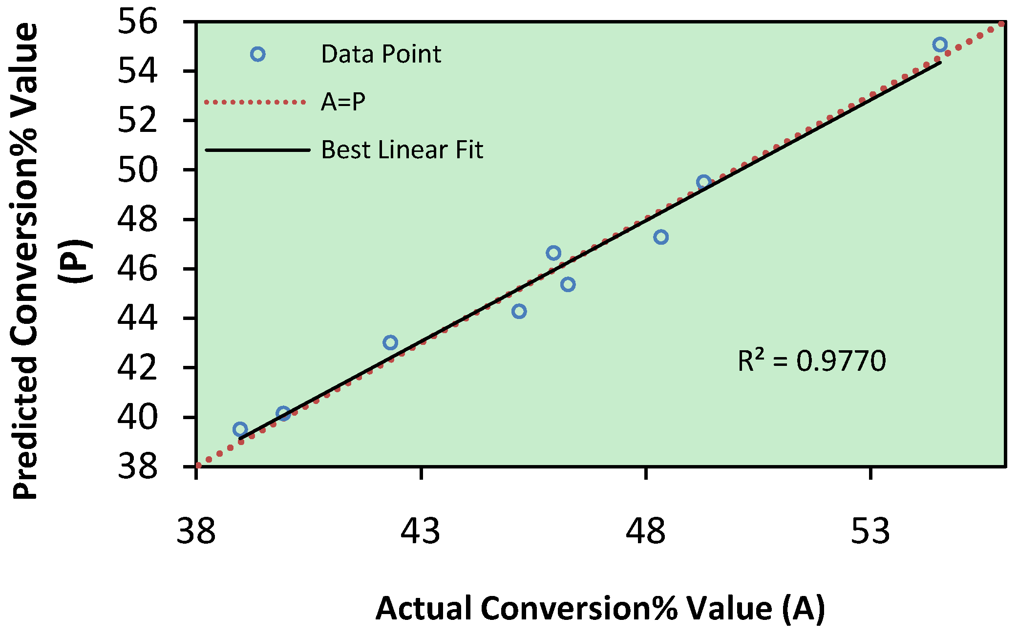
2.1. Analysis of Experimental Data and Prediction of Performance

| Run No. | Enzyme Amount (w/w %) | Reaction Time (hour) | Reaction Temperature (°C) | Molar Ratio of Substrates (mole) | Conversion % | |
|---|---|---|---|---|---|---|
| Actual | Predicted | |||||
| 1 | 0 | −1 | 0 | 0 | 48.34 | 47.29 |
| 2 | 1 | 0 | 0 | −1 | 46.27 | 45.37 |
| 3 | −1 | 1 | 0 | 1 | 45.18 | 44.28 |
| 4 | 1 | 1 | −1 | 0 | 42.32 | 43.01 |
| 5 | −1 | −1 | −1 | −1 | 38.98 | 39.51 |
| 6 | 1 | −1 | 1 | 1 | 54.54 | 55.07 |
| 7 | −1 | 0 | 1 | 0 | 45.95 | 46.64 |
| 8 | 0 | 0 | −1 | 1 | 49.29 | 49.50 |
| 9 | 0 | 1 | 1 | −1 | 39.94 | 40.15 |

2.2. Analysis of Variance (ANOVA)
| Source | Sum of Squares | Degree of Freedom | Mean Square | F Value | P Value | Remarks |
|---|---|---|---|---|---|---|
| Mean | 18751.65 | 1 | 18751.65 | - | - | - |
| Linear | 173.61 | 4 | 43.40 | 11.74 | 0.0175 | Suggested |
| 2FI | 12.22 | 3 | 4.07 | 1.59 | 0.5141 | Aliased |
| Residual | 2.56 | 0 | - | - | - | - |
| Total | 18940.05 | 9 | 2104.45 | - | - | - |
| Source | Sum of Squares | Degree of Freedom | Mean Square | F Value | P Value |
|---|---|---|---|---|---|
| Model | 184.07 | 5 | 36.81 | 25.54 | 0.0116 |
| Residual | 4.32 | 3 | 1.44 | - | - |
| Corrected Total | 188.39 | 8 | - | - | - |
| R-Squared | 0.9770 | Standard Deviation | 1.20 | ||
| Adjusted R2 | 0.9388 | Coefficient of variation % | 2.63 | ||
| Adequate Precision | 15.872 | Predicted Residual Error of Sum of Squares (PRESS) | 46.41 | ||
| Source | Coefficient Estimate | Sum of Squares | Degree of Freedom | Mean Square | F Value | P Value |
|---|---|---|---|---|---|---|
| Intercept | 47.17 | - | - | - | - | - |
| X1 | −2.40 | 34.66 | 1 | 34.66 | 24.04 | 0.0162 |
| X2 | 1.64 | 16.14 | 1 | 16.14 | 11.19 | 0.0442 |
| X3 | 2.17 | 28.25 | 1 | 28.25 | 19.60 | 0.0214 |
| X4 | 3.97 | 94.57 | 1 | 94.57 | 65.60 | 0.0039 |
| X22 | −2.29 | 10.46 | 1 | 10.46 | 7.25 | 0.0742 |

2.3. Optimization of Reaction and Model Validation
| Exp. | Optimal Conditions | Conversion % | |||||
|---|---|---|---|---|---|---|---|
| X1 | X2 | X3 | X4 | Actual | Predicted | Relative Deviation | |
| 1 | 5.50 | 14.06 | 61.00 | 2.00 | 47.34 | 48.49 | 2.37 |
| 2 | 5.50 | 14.00 | 60.83 | 2.00 | 46.27 | 48.44 | 4.48 |
| 3 | 5.50 | 14.44 | 61.00 | 2.00 | 49.94 | 48.42 | 3.14 |
3. Experimental
3.1. Materials
3.2. Method
| Variable | Units | Coded Level of Variable | |||
|---|---|---|---|---|---|
| −1 | 0 | 1 | |||
| X1 | Enzyme Amount | %w/w | 3 | 5 | 7 |
| X2 | Reaction Time | Hour | 8 | 16 | 24 |
| X3 | Reaction Temperature | °C | 55 | 60 | 65 |
| X4 | Molar ratio of substrates | OA:TEA (mole:mole) | 1:1 | 2:1 | 3:1 |
4. Conclusions
Acknowledgements
References
- Miao, Z.; Yang, J.; Wang, L.; Liu, Y.; Zhang, L.; Li, X.; Peng, L. Synthesis of biodegradable lauric acid ester quaternary ammonium salt cationic surfactant and its utilization as calico softener. Mater. Lett. 2008, 62, 3450–3452. [Google Scholar]
- Guo, X.F.; Jia, L.H. Synthesis and Application of Cationic Surfactants; Chemical Industry Press: Beijing, China, 2002. [Google Scholar]
- Waters, J.; Kleiser, H.H.; How, M.J.; Barratt, M.D.; Birch, R.R.; Fletcher, R.J.; Haigh, S.D.; Hales, S.G.; Marshall, S.J.; Pestell, T.C. A new rinse conditioner active with improved environmental properties. Tenside Surfact. Det. 1991, 28, 460–468. [Google Scholar]
- Puchta, R.; Krings, P.; Sandkuehler, P. A New Generation of Softeners. Tenside Surfact. Det. 1993, 30, 186–191. [Google Scholar]
- Levinson, M. Rinse-added fabric softener technology at the close of the twentieth century. J. Surfact. Deterg. 1999, 2, 223–235. [Google Scholar] [CrossRef]
- Ebrahimiasl, S.; Yunus, W.M.Z.W.; Kassim, A.; Zainal, Z. Prediction of grain size, thickness and absorbance of nanocrystalline tin oxide thin film by Taguchi robust design. Solid State Sci. 2010, 12, 1323–1327. [Google Scholar] [CrossRef]
- Tsai, H.H.; Wu, D.H.; Chiang, T.L.; Chen, H.H. Robust Design of SAW Gas Sensors by Taguchi Dynamic Method. Sensors 2009, 9, 1394–1408. [Google Scholar] [CrossRef]
- Joo, Y.K.; Zhang, S.H.; Yoon, J.H.; Cho, T.Y. Optimization of the Adhesion Strength of Arc Ion Plating TiAlN Films by the Taguchi Method. Materials 2009, 2, 699–709. [Google Scholar] [CrossRef]
- Bolboac, S.D.; Jäntschi, L. Design of experiments: Useful orthogonal arrays for number of experiments from 4 to 16. Entropy 2007, 9, 198–232. [Google Scholar] [CrossRef]
- Aggarwal, A.; Singh, H.; Kumar, P.; Singh, M. Optimizing power consumption for CNC turned parts using response surface methodology and Taguchi's technique--A comparative analysis. J. Mater. Process. Tech. 2008, 200, 373–384. [Google Scholar] [CrossRef]
- Benyounis, K.; Olabi, A. Optimization of different welding processes using statistical and numerical approaches-A reference guide. Adv. Eng. Softw. 2008, 39, 483–496. [Google Scholar] [CrossRef]
- Phadke, S.M. Quality Engineering Using Robust Design; Prentice Hall: Englewood Cliffs, NJ, USA, 1989. [Google Scholar]
- Kackar, R.N. Off-Line Quality Control, Parameter Design, and the Taguchi Method. J. Qual. Technol. 1985, 17, 176–188. [Google Scholar]
- Taguchi, G. Introduction to Quality Engineering; Asian Productivity Organization: Dearborn, MI, USA, 1986; Distributed by American Supplier Institute Inc. [Google Scholar]
- Bendell, A. Introduction to Taguchi Methodology. In Taguchi Methods: Proceedings of the 1988 European Conference; Elsevier Applied Science: London, England, 1988. [Google Scholar]
- ASI, Taguchi Methods: Implementation Manual; American Supplier Institute Inc (ASI): Dearborn, MI, USA, 1989.
- Taguchi, G.; Konishi, S. Orthogonal Arrays and Linear Graphs; American Supplier Institute Inc.: Dearborn, MI, USA, 1987. [Google Scholar]
- Muralidhar, R.V.; Chirumamila, R.R.; Marchant, R. A response surface approach for the comparison of lipase production by Candida Cylindracea using two different carbon sources. Biochem. Eng. J. 2001, 9, 17–23. [Google Scholar] [CrossRef]
- Anderson, M.J.; Whitcomb, P.J. RSM Simplified: Optimizing Processes Using Response Surface Methods for Design of Experiments; Productivity Press: New York, NY, USA, 2005. [Google Scholar]
- Myers, R.H.; Montgomery, D.C. Response Surface Methodology: Process and Product Optimization Using Designed Experiments; John Wiley & Sons,Inc: New York, NY, USA, 1995. [Google Scholar]
- Yadav, R.; Srivastava, D. Studies on the process variables of the condensation reaction of cardanol and formaldehyde by response surface methodology. Eur. Polym. J. 2009, 45, 946–952. [Google Scholar] [CrossRef]
- Hamzaoui, A.H.; Jamoussi, B.; M’nif, A. Lithium recovery from highly concentrated solutions: Response surface Methodology (RSM) process parameters optimization. Hydrometallurgy 2008, 90, 1–7. [Google Scholar] [CrossRef]
- Li, Y.; Lu, J. Characterization of the enzymatic degradation of arabinoxylans in grist containing wheat malt using response surface methodology. J. Am. Soc. Brew. Chem. 2005, 63, 171–176. [Google Scholar]
- Beg, Q.; Sahai, V.; Gupta, R. Statistical media optimization and alkaline protease production from Bacillus mojavensis in bioreactor. Process Biochem. 2003, 39, 203–209. [Google Scholar] [CrossRef]
- Yuan, X.; Liu, J.; Zeng, G.; Shi, J.; Tong, J.; Huang, G. Optimization of conversion of waste rapeseed oil with high FFA to biodiesel using response surface methodology. Renew. Energy 2008, 33, 1678–1684. [Google Scholar] [CrossRef]
- Liu, J.Z.; Weng, L.P.; Zhang, Q.L. Optimization of glucose oxidase production by Aspergillus Niger in a benchtop bioreactor using response surface methodology. World J. Micro. Biotech. 2003, 19, 317–323. [Google Scholar] [CrossRef]
- Krishna, S.H.; Sattur, A.P.; Karanth, N.G. Lipase-catalysed synthesis of isoamly isobutyrate-optimisation using a central composite rotatable design. Process Biochem. 2001, 37, 9–16. [Google Scholar] [CrossRef]
© 2011 by the authors; licensee MDPI, Basel, Switzerland. This article is an open access article distributed under the terms and conditions of the Creative Commons Attribution license ( http://creativecommons.org/licenses/by/3.0/).
Share and Cite
Masoumi, H.R.F.; Kassim, A.; Basri, M.; Abdullah, D.K. Determining Optimum Conditions for Lipase-Catalyzed Synthesis of Triethanolamine (TEA)-Based Esterquat Cationic Surfactant by a Taguchi Robust Design Method. Molecules 2011, 16, 4672-4680. https://doi.org/10.3390/molecules16064672
Masoumi HRF, Kassim A, Basri M, Abdullah DK. Determining Optimum Conditions for Lipase-Catalyzed Synthesis of Triethanolamine (TEA)-Based Esterquat Cationic Surfactant by a Taguchi Robust Design Method. Molecules. 2011; 16(6):4672-4680. https://doi.org/10.3390/molecules16064672
Chicago/Turabian StyleMasoumi, Hamid Reza Fard, Anuar Kassim, Mahiran Basri, and Dzulkifly Kuang Abdullah. 2011. "Determining Optimum Conditions for Lipase-Catalyzed Synthesis of Triethanolamine (TEA)-Based Esterquat Cationic Surfactant by a Taguchi Robust Design Method" Molecules 16, no. 6: 4672-4680. https://doi.org/10.3390/molecules16064672
APA StyleMasoumi, H. R. F., Kassim, A., Basri, M., & Abdullah, D. K. (2011). Determining Optimum Conditions for Lipase-Catalyzed Synthesis of Triethanolamine (TEA)-Based Esterquat Cationic Surfactant by a Taguchi Robust Design Method. Molecules, 16(6), 4672-4680. https://doi.org/10.3390/molecules16064672