Numerical Prediction of Entropy Generation in Separated Flows

Department of Mechanical Engineering, Hashemite University, Zarqa, 13115, Jordan
Entropy 2005, 7(4), 234-252; https://doi.org/10.3390/e7040234
Submission received: 17 July 2005
/
Accepted: 5 September 2005
/
Published: 6 October 2005
Abstract
:The present research investigates second law analysis of laminar flow over a backward facing step (BFS). Entropy generation due to separation, reattachment, recirculation and heat transfer is studied numerically. Local entropy generation distributions were obtained by solving momentum, energy, and entropy generation equations. The effect of dimensionless temperature difference number (τ) and Brinkman number (Br) on the total entropy generation number (Ns) was investigated. Moreover, the effect of Reynolds number (Re) on the value of Ns was reported. It was found that as Re increased the value of Ns increased. Also, as Br increased the value of Ns increased. However, it was found that as τ increased the value of Ns decreased. For the bottom wall of the channel, the maximum value of Ns occurs inside the recirculation zone and reduces to a minimum value at the point of reattachment point. Also, for Re ≥ 500, a second peak of entropy generation appears after the reattachment point. For the top wall of the channel, the value of Ns has a maximum value directly above the step and its value reduced downstream the step. The contribution of the top wall to Ns downstream the point of reattachment was relatively small.
Introduction
Heat Transfer and fluid flow processes are inherently irreversible, which leads to an increase in entropy generation and thus destruction of useful energy. The optimal second law design criteria depend on the minimization of entropy generation encountered in fluid and heat transfer processes.
In the last three decades several studies have focused on second law analysis of heat and fluid flow. Bejan [1, 2] showed that entropy generation in convective fluid flow is due to heat transfer and viscous shear stresses. Arpaci and Selamet [3] studied entropy generation in boundary layers. They showed that the entropy generation in boundary layers is due to temperature gradient and viscosity effects. San and Lavan [4] investigated the entropy generation for combined heat and mass transfer in a two dimensional channel. Also, numerical studies on the entropy generation in convective heat transfer problems were carried out by different researchers. Drost and White [5] developed a numerical solution procedure for predicting local entropy generation due to fluid impinging on a heated wall. Abu-Hijleh et al. [6, 7, and 8], studied entropy generation due to natural convection around a horizontal cylinder. Haddad et al. [9] considered the local entropy generation of steady two-dimensional symmetric flow past a parabolic cylinder in a uniform flow stream. However, very little work found in literature dealing with entropy generation in separated flows.
Separated flows, accompanied with heat transfer, are frequently encountered in various engineering applications, such as heat exchangers and ducts used in industrial applications. These separated flows are intrinsically irreversible because of viscous dissipation, separation, reattachment and recirculation that generate entropy. The flow over a backward facing step (BFS) was studied extensively to understand the physics of such separated flows. The BFS has the most features of separated flows, such as separation, reattachment, recirculation, and development of shear layers. However, most of the published work on BFS has been extensively investigated, from a fluid mechanics perspective or from a heat transfer perspective. For example, Armaly et al. [10] studied laminar, transition, and turbulent isothermal flow over a BFS experimentally. Also, numerical studies in the laminar regime for isothermal flow were conducted by Armaly et al. [10] and by Durst and Periera [11]. Additional numerical work for a two-dimensional isothermal flow over a BFS was conducted by Gartling [12], Kim and Moin [13], and Sohn [14]. Flow over a BFS with heat transfer was conducted by Vradis et al. [15], Pepper et al. [16], and Lin et al. [17]. Also, studies on three-dimensional effects on flow characteristics, over a BFS, were also carried out [18, 19, 20, and 21].
Review of existing literature reveals no work analyzing flow over BFS with heat transfer from a second law point of view. This problem needs to be analyzed from a second law perspective to evaluate the performance of flows experiencing separation, reattachment, and vortices in conserving useful energy. Thus, the present work was carried out to gain deeper understanding of the destruction of the useful energy encountered in a separated flow accompanied with heat transfer. The present research investigates, numerically, entropy generation due to heat transfer fluid flow over a BFS.
Governing Equations
The dimensionless continuity, momentum, energy, and entropy generation equations in Cartesian coordinates are given as [22, 23]:
![Entropy 07 00234 i001]()
![Entropy 07 00234 i002]()
![Entropy 07 00234 i003]()
![Entropy 07 00234 i004]()
![Entropy 07 00234 i005]() where x, y are the non dimensional coordinates, with respect to the channel height H, The other dimensionless quantities are defined as:
where x, y are the non dimensional coordinates, with respect to the channel height H, The other dimensionless quantities are defined as:
![Entropy 07 00234 i006]() where U is the average velocity of the incoming flow at the step, Tw is the temperature of the wall directly at step, and Tcl is the temperature of the incoming flow. The non-dimensional numbers are given as: Reynolds number Re = , Prandtl number Pr = , entropy generation number Ns = , Brinkman number Br = ,and the dimensionless temperature parameter τ = .
where U is the average velocity of the incoming flow at the step, Tw is the temperature of the wall directly at step, and Tcl is the temperature of the incoming flow. The non-dimensional numbers are given as: Reynolds number Re = , Prandtl number Pr = , entropy generation number Ns = , Brinkman number Br = ,and the dimensionless temperature parameter τ = .


Equation 4 was derived by assuming that the temperature difference (Tcl-Tw) is not relatively high such that constant fluid physical properties assumption applies.
Problem Description and Boundary Conditions
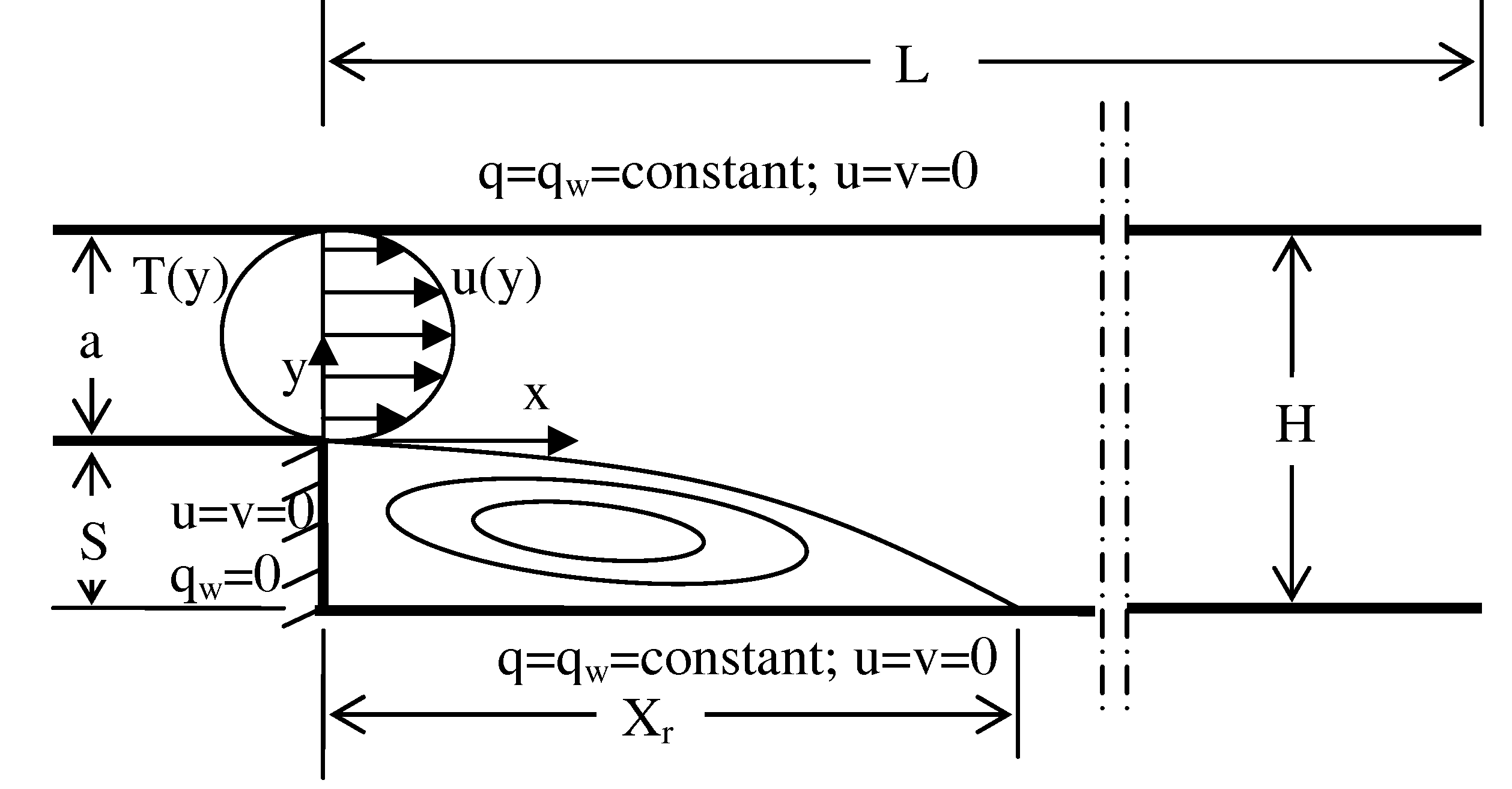
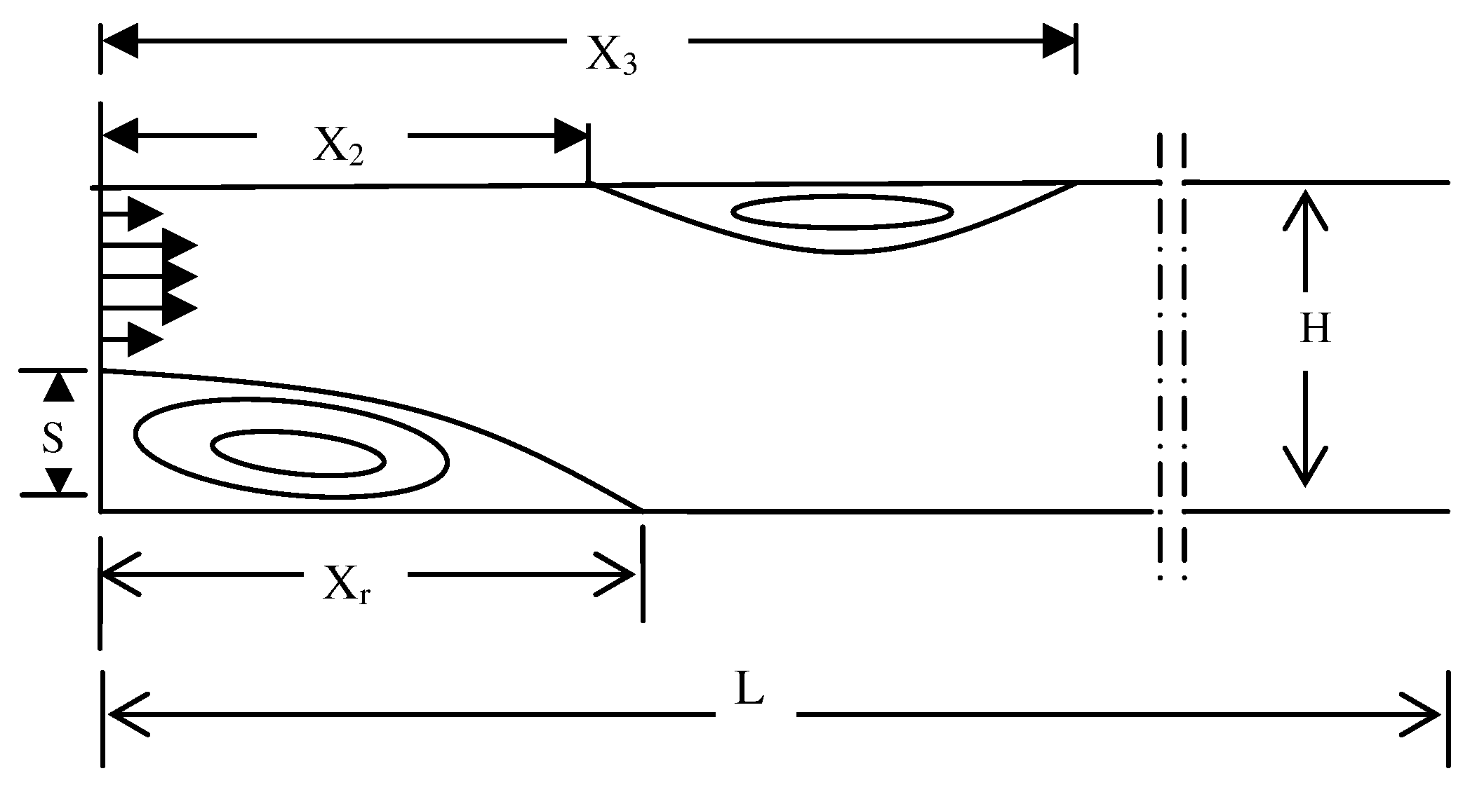
The basic flow configuration, under study, is shown in Fig. 1. The expansion ratio (S/H) is set to 1/2. The channel length (L) is set to 30H. The flow is considered to be two-dimensional, laminar, steady, constant fluid properties, and incompressible.
The flow at the inlet, at x=0, is assumed hydro-dynamically fully developed, where the dimensionless parabolic velocity distribution is given as:
A no-slip velocity boundary condition is applied along the top wall, bottom wall, and the vertical wall of the step, see Fig. 1. A fully developed outlet velocity boundary condition is assumed:
![Entropy 07 00234 i007]()

Also, the temperature profile at the inlet is assumed to be fully developed and is given as:
![Entropy 07 00234 i008]()

An adiabatic boundary condition is imposed on the vertical wall of the step, i.e. x= 0. However, a constant heat flux, , is enforced along the top and the bottom channel walls downstream the step.
The value of the heat flux is set equal to:
![Entropy 07 00234 i009]()

Equation 9 can be expressed in terms of non-dimensional temperature as:
![Entropy 07 00234 i010]()

Numerical Implementation
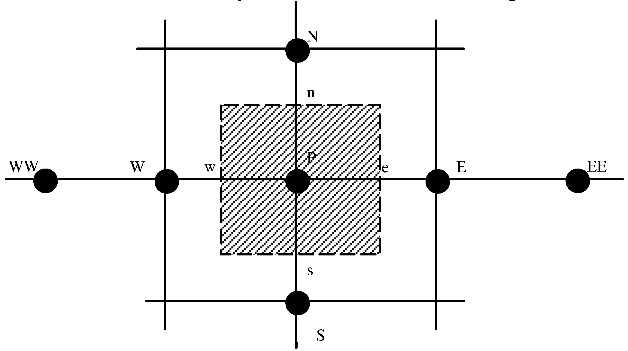
Equations 1, 2, 3, and 4, with the corresponding boundary conditions, are solved using the finite volume approach. The computational flow domain is decomposed into a set of non overlapping control volumes surrounding a grid node, as shown by the dotted lines in Fig. 2.
The governing equations are integrated over each control volume and are discritized in terms of the values at a set of nodes defining the computational mesh (E, W, N, and S in Fig. 2). The SIMPLE algorithm [25] is used as the computational algorithm. For full details of the method see references [25, 26]. The diffusion term, in Eqs. 2, 3, and 4, is approximated by second-order central difference which gives very stable solution. However a hybrid differencing scheme is adopted for the convective terms, which makes the coefficients of the resulting finite volume equations always positive that satisfies the diagonally dominant condition [25, 26]. This scheme utilizes the favorable properties of the upwinding differencing scheme and central differencing scheme [25, 26]. This scheme is highly used in CFD packages and proved to be very useful for predicting physical problems [26].
A fine grid is used in the regions near the point of reattachment to resolve the steep velocity gradients while a coarser grid is used far the downstream. This is done using a grid stretching technique that results in considerable savings in terms of the grid size and thus in computational time. The grid stretching method is done by transforming the uniform spacing grid points, in the x direction, into a non uniform grid, by using the following transformation [24]
![Entropy 07 00234 i011]() where x is the location of non uniform stretched grid points, X is the location of the non-stretched grid points and A is a constant given by [24]:
where x is the location of non uniform stretched grid points, X is the location of the non-stretched grid points and A is a constant given by [24]:
![Entropy 07 00234 i012]()


The parameter β is a stretching constant, D is the locations of grid clustering, and L is the channel length. The grid stretching is used in x direction; however, a uniform grid is used in y direction. In the y direction steep velocity gradients take place next to the top and bottom walls. So, sufficient grid points need to be used nearby. Besides, at the point of separation a fine grid need to be used. Moreover, inside the primary recirculation zone and secondary recirculation zone a fine grid need to be used to resolve the velocity gradients inside these zones. So, it is clearly evident that the flow all over the y direction experience steep velocity gradients. For that reason a uniform grid is used to distribute the grid points evenly in the y direction between these areas that experience steep velocity gradients. The grid independence study gives very accurate solution by using such uniform grid in the y direction, as will be shown in the next section.
The final discretized algebraic finite volume equations are written into the following form:
where P, W, E, N, S denotes cell location, west face of the control volume, east face of the control volume, north face of the control volume and south face of the control volume, respectively. The symbol φ in Eq. 13 holds for u, v, or T. The resulted algebraic equations are solved with tri-diagonal matrix algorithm (Thomas algorithm) with the line-by-line relaxation technique. The convergence criteria were defined by the following expression:
![Entropy 07 00234 i013]() where resid is the residual; M and N are the number of grid points both in both the axial and the vertical directions, in the computational plane, respectively.
where resid is the residual; M and N are the number of grid points both in both the axial and the vertical directions, in the computational plane, respectively.
aEφE − aWφW + aPφP = aNφN + aSφS

After the temperature and velocity fields are obtained, by solving Eq. 13, Eq. 5 is used to solve for the entropy generation number at each grid point in the flow domain. These point entropy generation numbers are used to generate further useful total entropy generations in the flow domain. For example, the total entropy generation number along the top and the bottom wall can be found by using the following two equations respectively:
![Entropy 07 00234 i014]()
![Entropy 07 00234 i015]()


Because of the non-uniformity of the grid in the stream wise direction, the integrations, in Eq. 15 and Eq. 16, were carried out using a cubic spline interpolation technique. Then, the Simpson’s rule of integration was employed.
The rate of entropy generation number at each cross section, Ns (x), is calculated by using the following equation:
![Entropy 07 00234 i016]()

The Simpson’s rule of integration was employed in the y-direction without using cubic splines since the grid is uniform in the y direction.
The total entropy generation over the entire flow domain is calculated using the following equation:
![Entropy 07 00234 i017]()

The magnitude of the Nusselt number can be expressed as:
![Entropy 07 00234 i018]() where h is the convective heat transfer coefficient given by
where h is the convective heat transfer coefficient given by
![Entropy 07 00234 i019]()


Equation 20 can be expressed in terms of non-dimensional temperature as:
![Entropy 07 00234 i020]()

By Equating Eq. 10 and Eq. 21, and noting that (θcl − θw) = 1, then the Nusselt number can be expressed as:
![Entropy 07 00234 i021]()

Grid testing
Extensive mesh testing was performed to guarantee grid independence solution. Eight different meshes were used for the grid independence study as shown in Table 1. According to the experiment of Armaly et al. [10], and previous published numerical work [12, 13, 15, 16], two recirculation flow zones are encountered for Re = 800; See Fig 3. The primary recirculation zone occurs directly downstream the step at the bottom wall of the channel, whereas the other secondary recirculation zone exists along the top wall. However, for lower Reynolds numbers, such as Re=400, only the bottom recirculation zone appears. The Re = 800 was used, in the present work, to perform grid independence because it has been accepted as a benchmark problem by the “Benchmark Solutions to Heat Transfer Problems” organized by the K-12 committee of the ASME [15,16]. The BFS problem under study was tested for calculating reattachment length (Xr), X2, and X3. Moreover, the Nusslet number over the top wall at the outflow of the channel was calculated.
Code Validation
The present numerical solution is validated by comparing present results, for Re = 800, with the experiment of Armaly et al. [10] and with other numerical published work [12, 13, 15, and 16]. As shown in Table 2, the present work predictions are very close to the other numerical published work results. However, all of the numerical published work, including present work, under estimates the reattachment length. According to Armaly et al. [10], the flow at Re=800 has three dimensional features. So, the under estimation of Xr, by all numerical published work are due to two-dimensional flow assumption embedded in the numerical solutions [15]. More specifically, it is due to the side wall induced three dimensional effects [18, 19, and 20]. According to the work of Williams and Baker [19], the interaction of a wall jet at the step near to the side walls with the mainstream flow causes a formation of three-dimensional flow structure in a region of essentially two-dimensional flow near the mid plane of the channel. Thus, the under estimation of the reattachment length at high values of Reynolds number is due to the influence of the side wall three dimensional effects [18,19]. In particular, Barkely et al. [20] have shown that in the absence of sidewalls the transition to three dimensional flow structures appears at a higher value of Reynolds number around 1000.
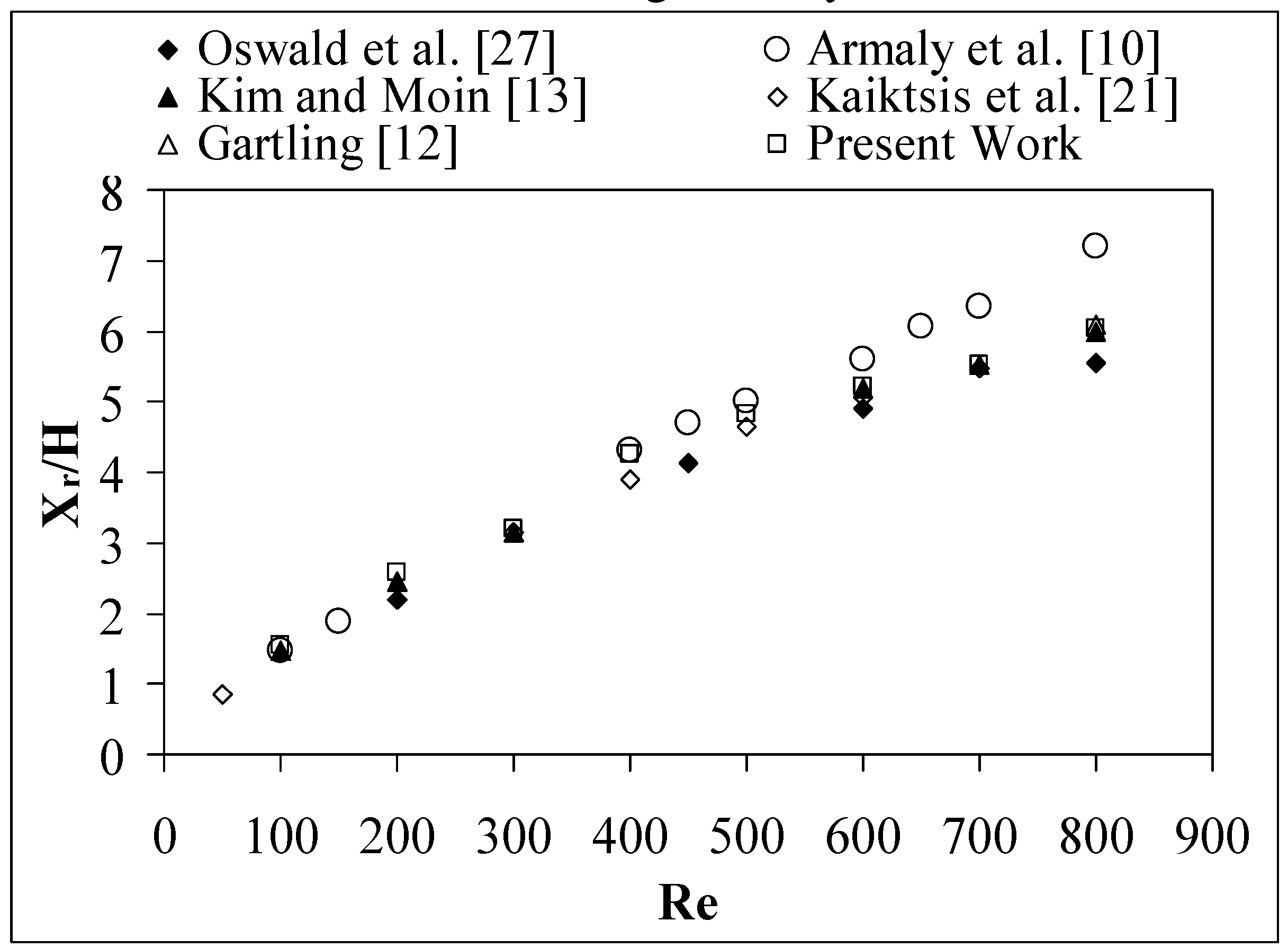
On the other hand, further comparison between present results and previously published work for the whole range of Reynolds number is given in Fig. 4. The figure shows an excellent agreement between our results and the experiment of Armaly et al. [10] for Re ≤600. Also, it shows an excellent agreement with all numerical published work for the entire range of Reynolds number.
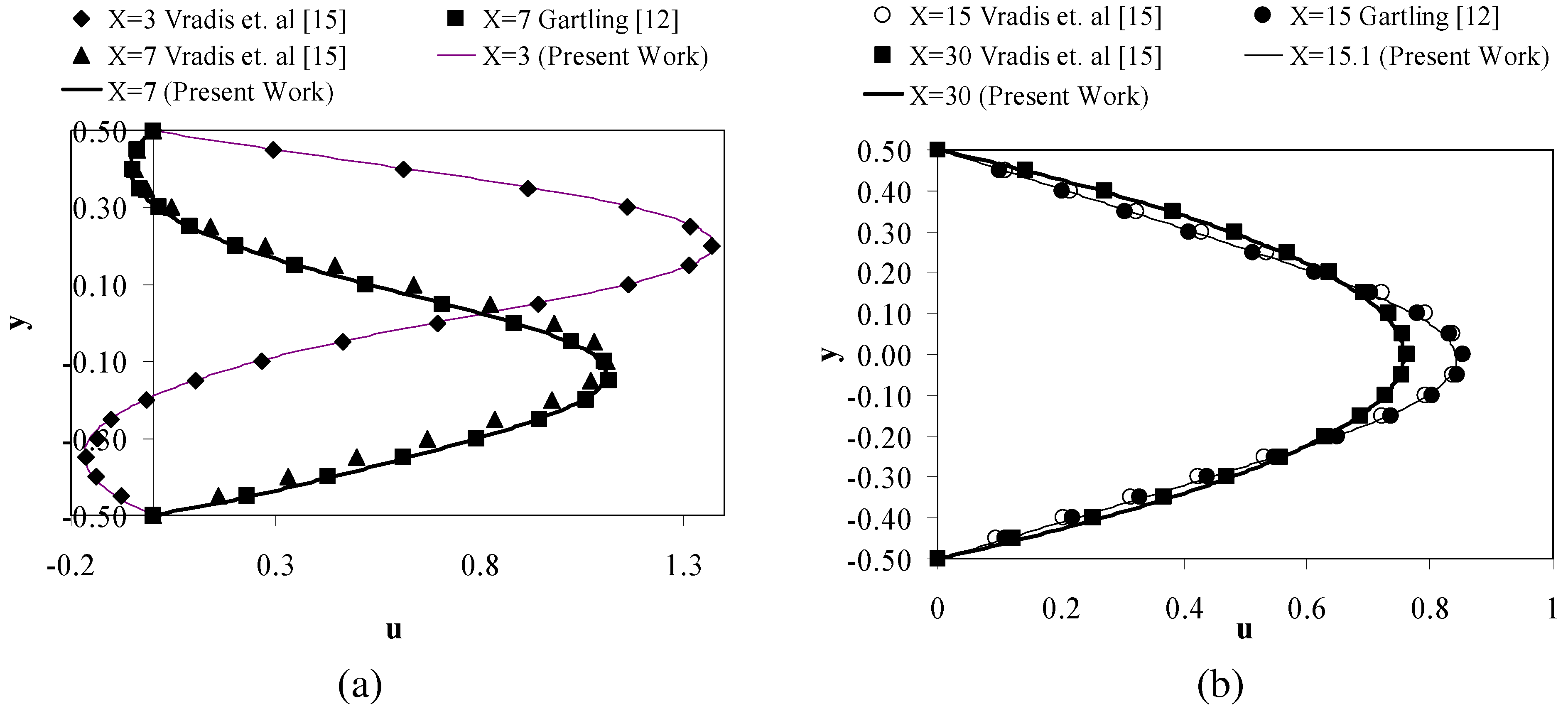
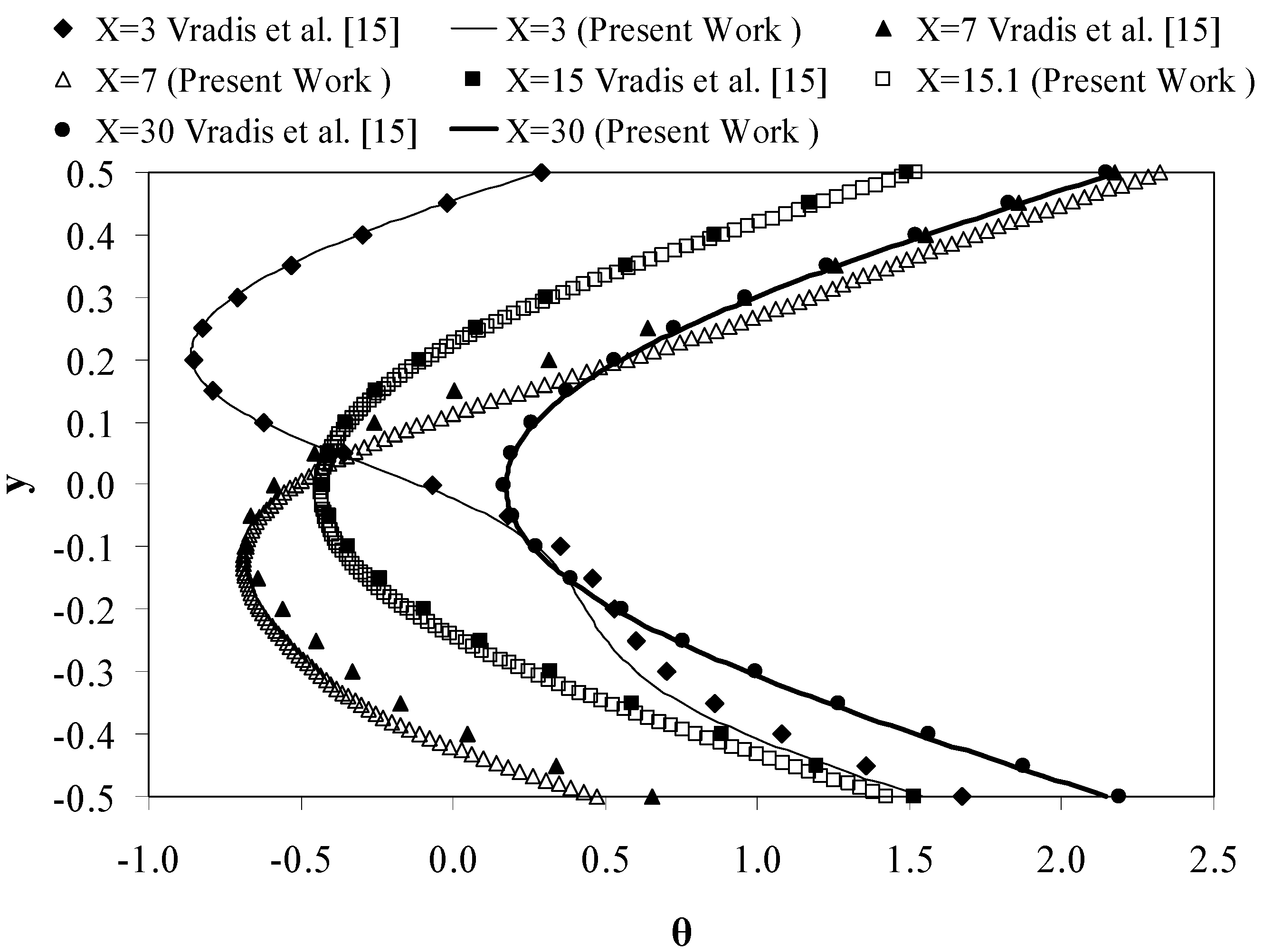
Figure 5 compares x component of velocity with the work of Gartling [12] and Vradis et al. [15]. Also, Fig. 6 compares temperatures profiles with the work of Gartling [12] and Vradis et al. [15]. As shown in Fig. 5 and Fig. 6, there is a good agreement between present work and the previous published work.
Results and Discussion
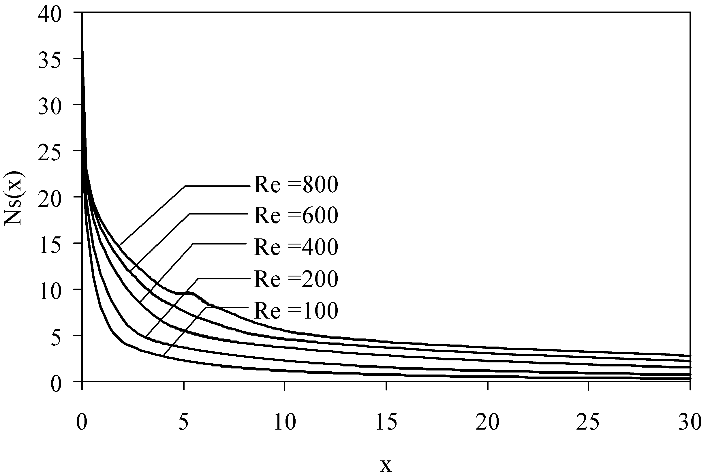
The present research results are presented for a Reynolds number range between 100 and 800. The Prandtl number is kept constant at 0.71 to guarantee constant fluid physical properties for moderate and small values of temperature difference (Tcl -Tw). The variation of cross-sectional entropy generation number, Ns(x) given in Eq. 17, along the channel length is shown in Fig. 7. For all Reynolds numbers, the maximum Ns(x) occurs directly at the step location (x=0) and the value of Ns(x) decreases down stream the step. The reason for having maximum values of Ns(x) at x =0 is due to two factors. First is the separation that occurs at x = 0, which produces large velocity gradients. These velocity gradients increase the viscous contribution to Ns(x). Second is the adiabatic vertical step wall which generates high temperature spots. These spots increase the conduction contribution to Ns(x). The dependence of Ns(x) on Reynolds number is illustrated in the same figure. There is an increase in Ns(x) with Reynolds number due to the increase in velocity gradients. Moreover, the figure shows that above x=10 the value of Ns(x) does not change significantly, because the flow is progressing toward the fully developed condition. By reaching this condition the viscous and conduction contributions become, approximately, constant. Figure 7 presents results for Br = 1 and τ = 2, however, similar behaviors are obtained for different combinations for Br and τ.
Figure 8 shows the axial variation of Ns along the bottom wall of the channel for Re=400 and for various Brinkman numbers. The minimum value of Ns occurs at x = 0, at the bottom left corner, since at this point there is no motion and no heat transfer is taking place. Also, Fig. 8 shows that the maximum value of Ns occurs inside the recirculation zone and then it drops sharply to a very low value at the point of reattachment. This behavior can be explained by noting that the vortices increase dramatically inside the recirculation zone, which tends to maximize the viscous contribution to Ns in this zone. However, at the point of reattachment no shear stresses are taking place, which diminish the viscous contribution and leave only the conduction contribution to Ns.
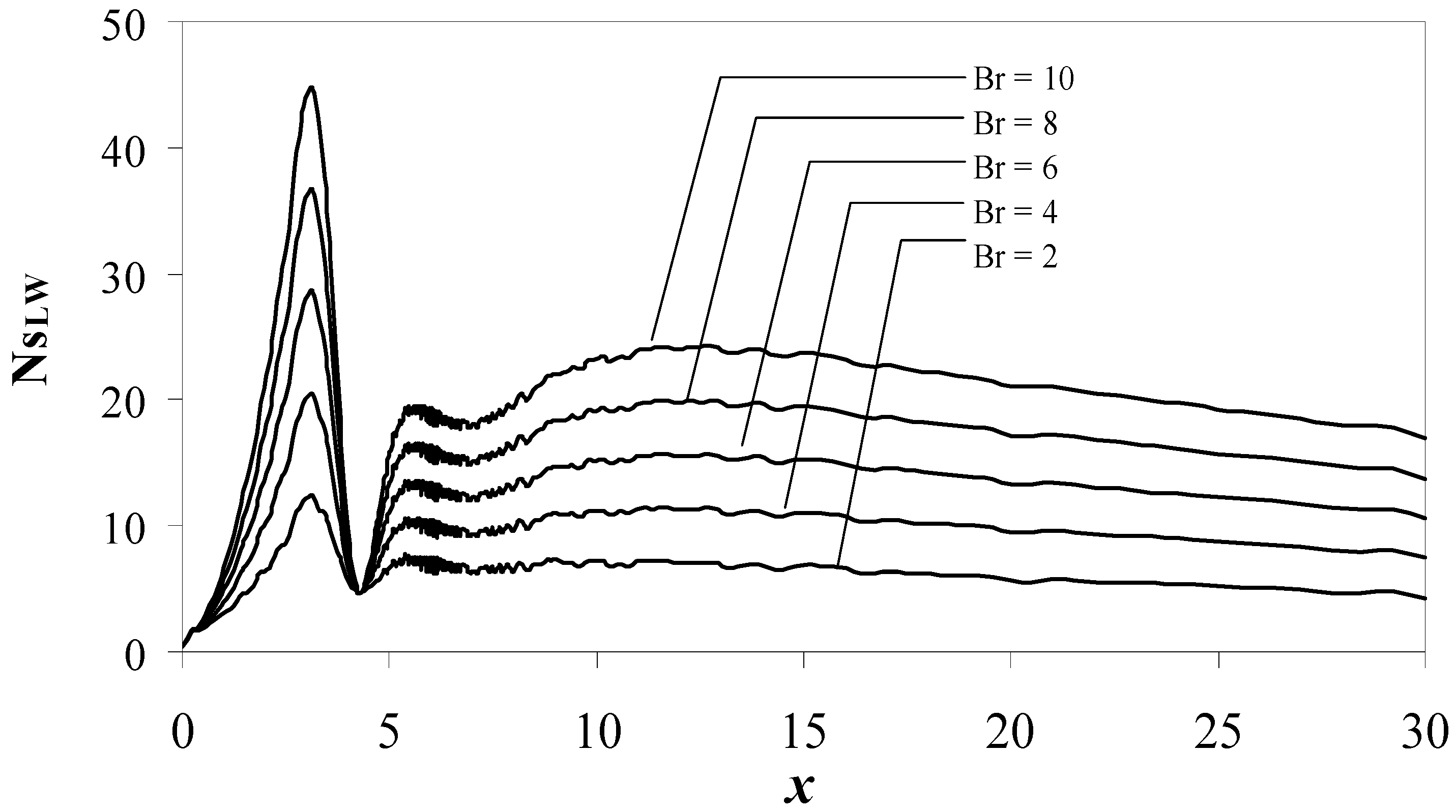
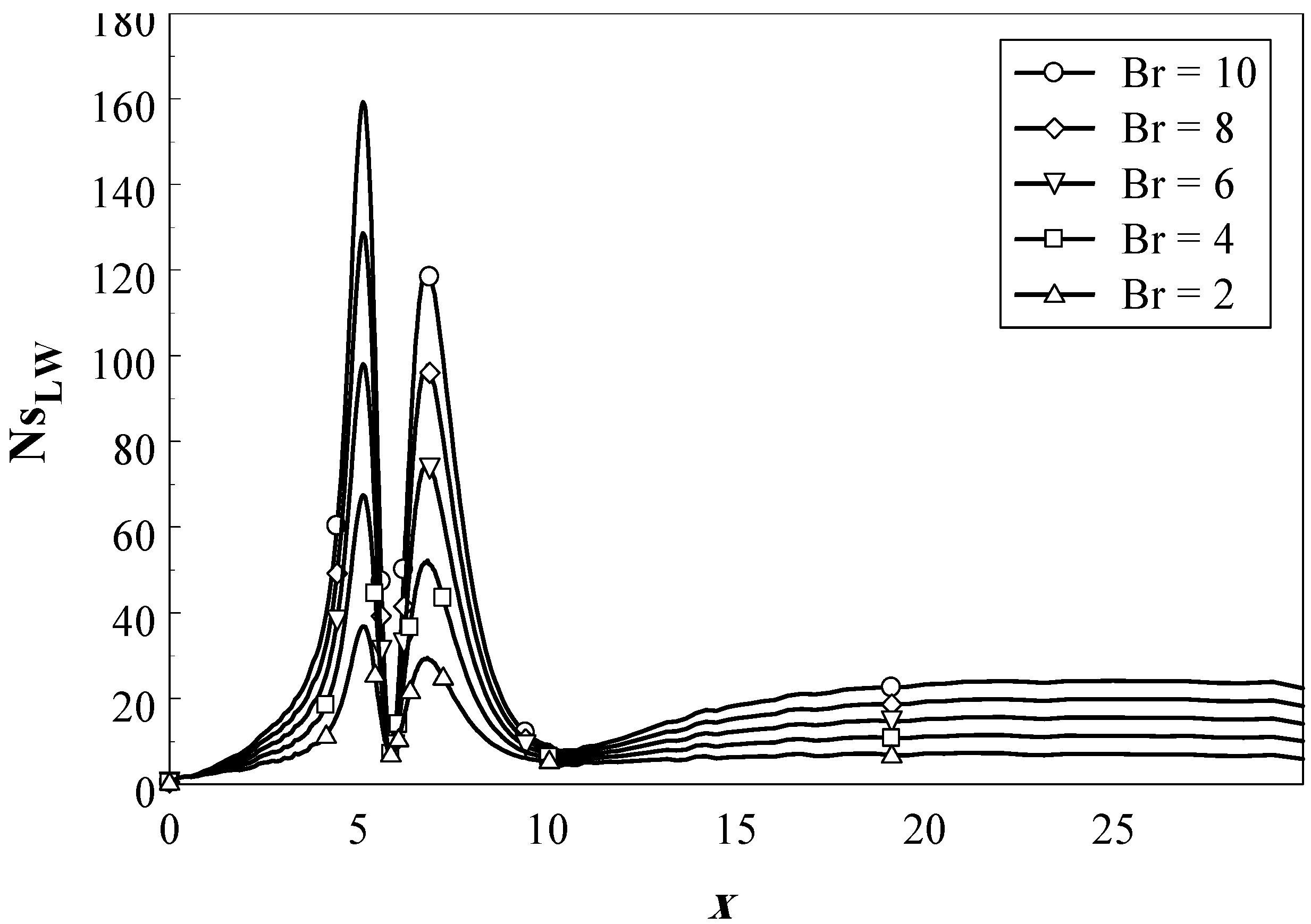
Figure 8 shows that at the point of reattachment the value of Ns is independent of the Brinkman number because there is no viscous contribution. Similar behaviors are also shown in Fig. 9 and Fig. 10 for Re = 600 and 800 respectively. However, Fig. 9 and Fig. 10 reveal new behavior that is not found in Fig. 8. This behavior is the appearance of a second peak zone after the point of reattachment. The beginning of the second peak zone occurs when the secondary recirculation bubble, on the top wall of the channel, appears. Also, the end of the second peak zone occurs when the top recirculation bubble disappears.
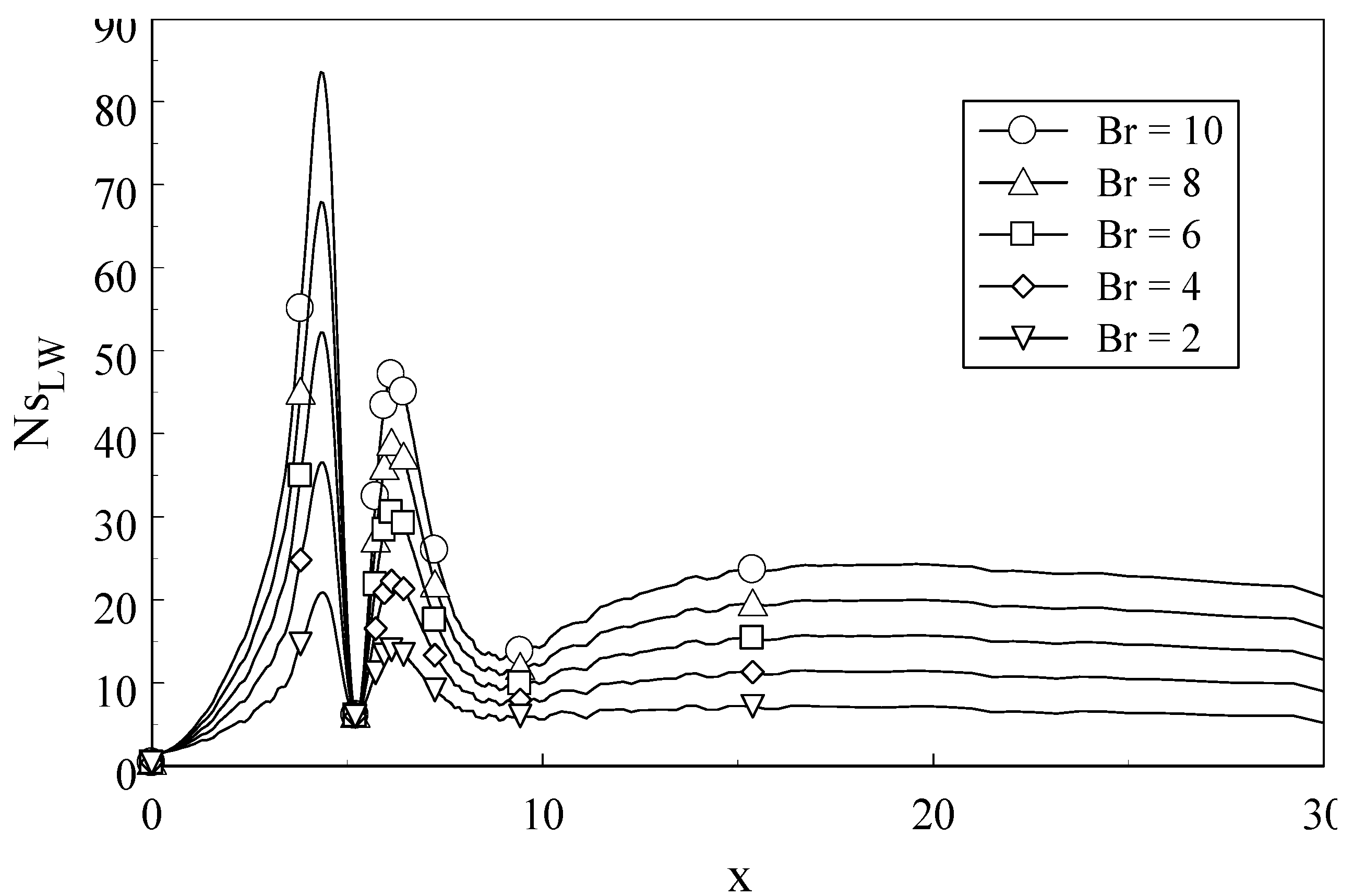
Note that Fig. 10 shows that the end of the second peaks zone is around 10 which is approximately the value of X3, see Table 2. Thus, it is very clearly that this second peak zone is related to secondary recirculation bubble. This recirculation bubble does not influence the value of Ns on the top wall of the channel; See Fig. 11. However, its main effect is on narrowing down the flow passage between the top secondary bubble and the bottom wall of the channel; See Fig 12. This would increase velocity gradients between the top secondary recirculation bubble and the bottom wall especially at the bottom wall due to the additional effect of the no-slip boundary condition. These high values of velocity gradients at the wall are responsible for high rates of entropy generation numbers that cause emerge of the second peak zone. Thus, it can be concluded that the effect of the top recirculation zone is very crucial in increasing local rates of entropy generation on the bottom wall of the channel and accordingly the total rates of entropy generation over the entire flow domain. Thus, any second law analysis improvement of the problem in hand must take into account the secondary recirculation zone. Note that the second peak zone only appears for Re ≥ 500.
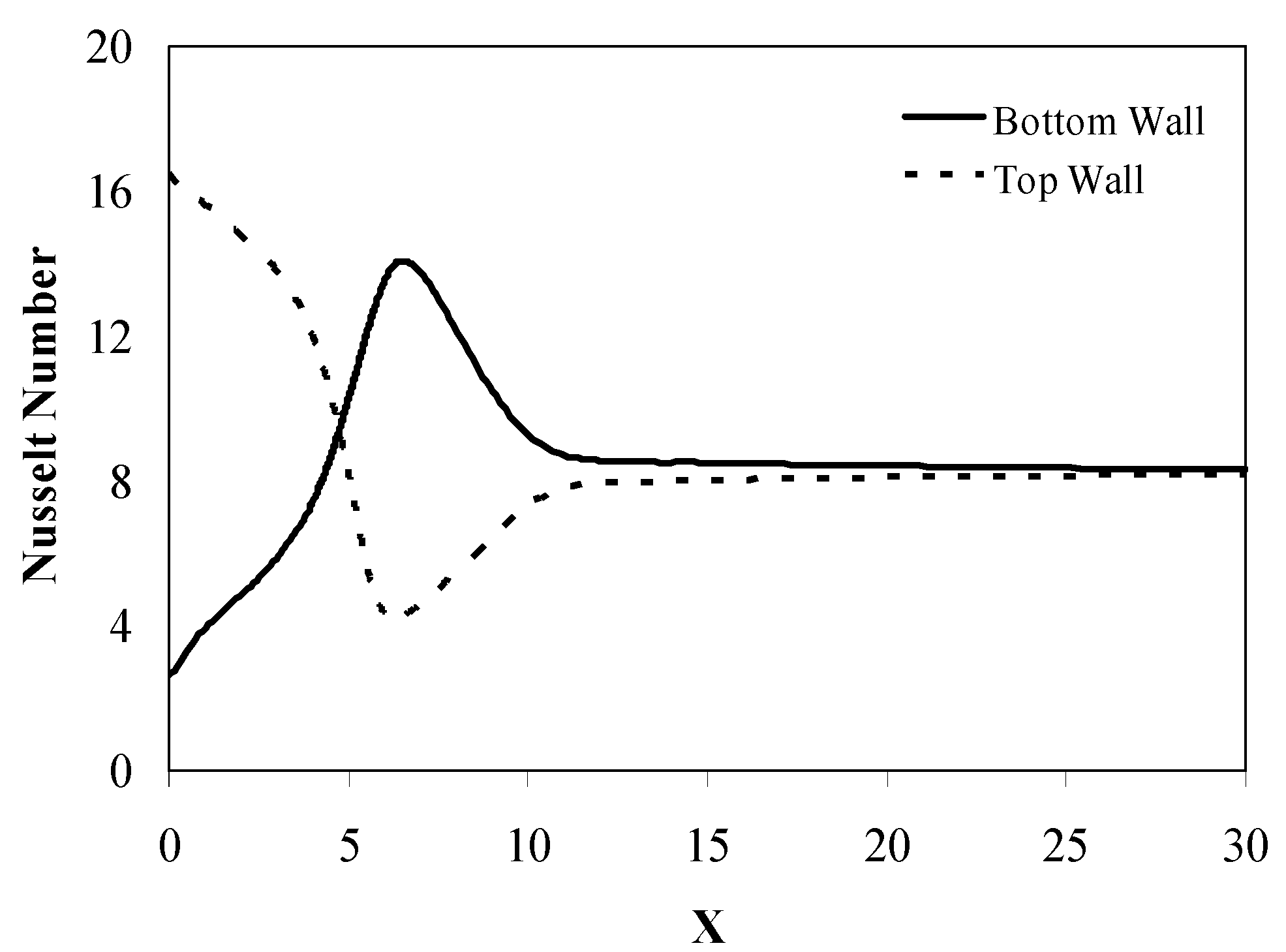
Figure 11 shows the Ns variation along the top wall of the channel, where a maximum value is detected at x = 0. The reason for having maximum values of Ns at the beginning of the top wall is the development of the viscous boundary layer. Also, the high values of heat transfer rate, where the highest local Nusselt number is recorded at the beginning of the top wall, see Fig. 13. Also, the figure shows that after the point of reattachment the value of Ns drops to very low values.
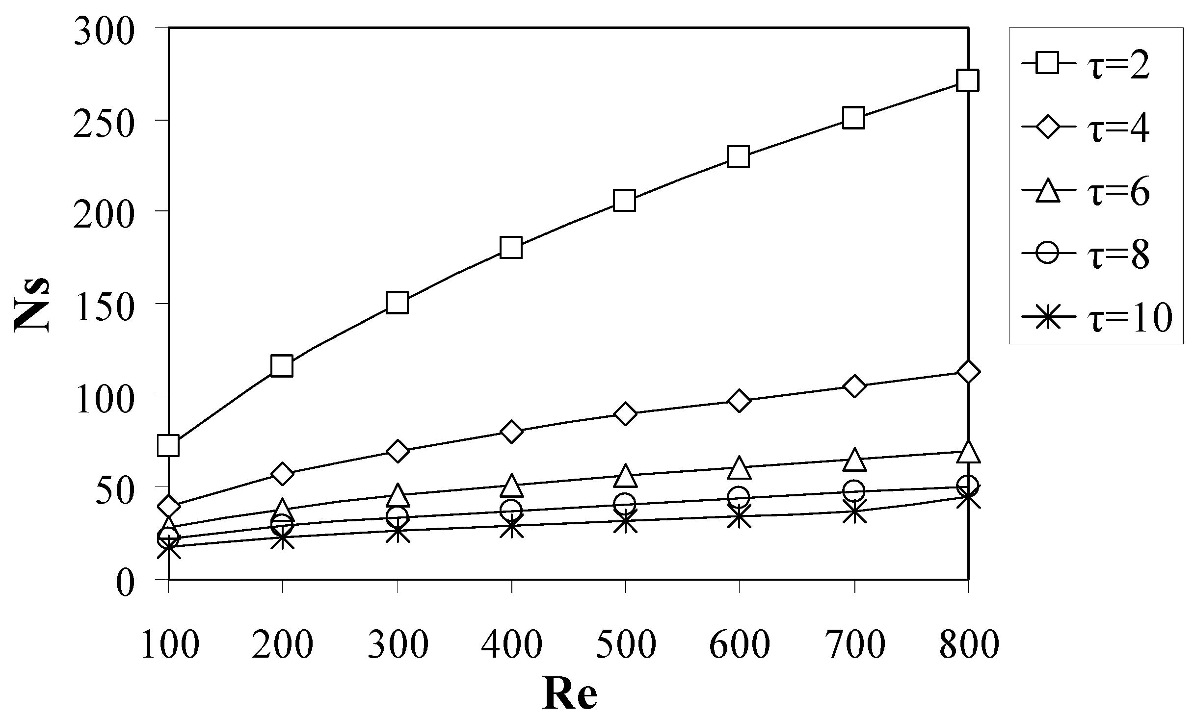
Figure 14 shows the effect of Reynolds number on the total entropy generation number (Ns). The value of Ns increases with Reynolds number for the whole range of Brinkman numbers. The increase in Reynolds number leads to an increase in viscous and conduction contribution to Ns. Also, Fig. 15 shows the variation of Ns with Reynolds number for different values of τ. The value of Ns increases with Reynolds number for the whole range of τ. However, the Ns is decreased as the values of τ are increased, because the temperature difference between the heated wall and the incoming flow stream decreases.
It can be concluded from the present results that the bad regions that have high values of Ns are the insulated step wall, separation point and the recirculation zones. The high production of Ns in these regions needs to be controlled to reduce entropy generation and thus conserving useful energy. Possible control methods are using suction/blowing at the top and at the bottom walls or imposing magnetic fields at the top and at the bottom walls.
Conclusion
Entropy generation in flow over a backward facing step (BFS) was calculated numerically. The results show that as Re increased the value of Ns increased. Also, as Br increased the value of Ns increased. The value of Ns decreased as τ increased. The value of the Ns(x) has a maximum value at the section where the flow separated and its value reduced as we moved downstream the step. It was found that for the lower wall the maximum value of Ns occurs inside the recirculation zone. On the top wall, the value of Ns, has a maximum value at the section, where the flow separated, and its value reduced as we moved downstream the step. The contribution of the top wall to Ns downstream the point of reattachment was relatively small. The results show that the top secondary recirculation zone increase entropy generation on the bottom wall of the channel when the top secondary bubble arises and has a negligible effect on the entropy generation on the top wall of the channel. The results obtained are an important step to devise methods for reduction of entropy generation to have a second law efficient separated flow.
Nomenclature
| A | Constant in the grid stretching equation |
| a | Upstream channel height |
| Br | Brinkman number |
| D | Location of grid clustering |
| H | Downstream channel height |
| h | local convection heat transfer coefficient |
| k | Thermal conductivity |
| L | Length of the channel |
| M | Number of points in horizontal direction |
| N | Number of points in vertical direction |
| Nu | Nusselt number |
| Ns | Total entropy generation number |
| p | Pressure |
| Pr | Prandtl number |
| Re | Reynolds number |
| U | Bulk velocity at inlet |
| u | x component of velocity |
| v | y component of velocity |
Heat flux at the top and bottom wall | |
| S | Step height |
Volume rate of entropy generation | |
| T | Temperature |
| Tw | Wall temperature |
| Tb | Bulk temperature |
| X2 | Beginning of the secondary recirculation bubble |
| X3 | End of the secondary recirculation bubble |
| Xr | Reattachment length |
Greek Letters
| α | Thermal diffusivity |
| β | Clustering parameter |
| θ | Dimensionless temperature |
| µ | Dynamic viscosity |
| ν | Kinematic viscosity |
| ρ | Density |
| τ | Dimensionless temperature parameter |
Subscripts
| b | Bulk value |
| cl | Centre line at inlet section |
| cond | Conduction |
| LW | Bottom wall |
| tot | Total |
| UW | Top wall |
| vis | Viscous |
| w | Wall |
Superscripts
| * | Dimensional quantities |
References
- Bejan, A. A study of entropy generation in fundamental convective heat transfer. J. Heat Transfer 1979, 101, 718–725. [Google Scholar] [CrossRef]
- Bejan, A. The thermodynamic design of heat and mass transfer processes and devices. J. Heat and Fluid Flow 1987, 8(4), 258–275. [Google Scholar] [CrossRef]
- Arpaci, V.S.; Selamet, A. Entropy production in boundary layers. J. Thermophysics and Heat Transfer 1990, 4, 404–407. [Google Scholar]
- San, J.Y.; Lavan, Z. Entropy generation in convective heat transfer and isothermal convective mass transfer. J. Heat Transfer 1987, 109, 647–652. [Google Scholar] [CrossRef]
- Drost, M.K.; White, M.D. Numerical prediction of local entropy generation in an impinging jet. J. Heat Transfer 1991, 113, 823–829. [Google Scholar] [CrossRef]
- Abu-Hijleh, B.; Abu-Qudais, M.; Abu Nada, E. Entropy generation due to laminar natural convection from a horizontal isothermal cylinder. J. Heat Transfer 1998, 120, 1089–1090. [Google Scholar] [CrossRef]
- Abu-Hijleh, B.; Abu-Qudais, M.; Abu Nada, E. Numerical prediction of entropy generation due to natural convection from a horizontal cylinder. Energy 1999, 24, 327–333. [Google Scholar] [CrossRef]
- Abu-Hijleh, B.; Jadallah, I.N.; Abu Nada, E. Entropy generation due to natural convection from a horizontal isothermal cylinder in oil. International Communications in Heat and Mass Transfer 1998, 25(8), 1135–1143. [Google Scholar] [CrossRef]
- Haddad, O.M.; Abu-Qudais, M.; Abu-Hijleh, B.A.; Maqableh, A.M. Entropy generation due to laminar forced convection flow past a parabolic cylinder. International Numerical Methods for Heat and Fluid Flow 2000, 7, 770–779. [Google Scholar] [CrossRef]
- Armaly, B.F.; Durst, F.; Pereira, J.C.F.; Schönung. Experimental and theoretical investigation of backward-facing step flow. J. Fluid Mechanics 1983, 127, 743–496. [Google Scholar] [CrossRef]
- Durst, F.; Pereira, J.C.F. Time-dependent laminar backward-facing step flow in a two-dimensional duct. J. Fluid Engineering 1988, 110, 289–296. [Google Scholar] [CrossRef]
- Gartling, D.K. A test problem for outflow boundary condition-Flow over a backward facing step. Int. J. Num. Methods Fluids 1990, 11, 953–967. [Google Scholar] [CrossRef]
- Kim, J.; Moin, P. Application of a fractional-step method to incompressible Navier-Stokes Equations. J. Computational Physics 1985, 59, 308–323. [Google Scholar] [CrossRef]
- Sohn, J. Evaluation of FIDAP on some classical laminar and turbulent Benchmarks. In J. Num. Methods Fluids 1988, 8, 1469–1490. [Google Scholar] [CrossRef]
- Vradis, G.C.; Outgen, V.; Sanchez, J. Heat transfer over a backward-facing step: Solutions to a benchmark. In Benchmark Problems for Heat Transfer Codes ASME 1992; HTD-Vol. 222, 1992; pp. 27–34. [Google Scholar]
- Pepper, D.W.; Burton, K.L.; Bruenckner, F.P. Numerical Simulation of Laminar Flow with Heat Transfer over a backward facing step. In Benchmark Problems for Heat Transfer Codes ASME 1992; HTD-Vol. 222, 1992. [Google Scholar]
- Lin, J.T.; Armaly, B.F.; Chen, T.S. Mixed convection in buoyancy-assisting vertical backward-facing step flows. Int. J. Heat and Mass Transfer 1990, 33(10), 2121–2132. [Google Scholar] [CrossRef]
- Tylli, N.; Kaiktsis, L.; Ineichen, B. Sidewall effects in flow over a backward-facing step: Experiments and numerical solutions. Physics fluids 2002, 14(11), 3835–3845. [Google Scholar] [CrossRef]
- Williams, P. T.; Baker, A.J. Numerical Simulation of laminar flow over a 3D backward-facing step. Int. J. Num. Methods Fluids 1997, 24, 1–25. [Google Scholar] [CrossRef]
- Barkely, D.; Gabriela, M.; Gomes, M.; Henderson, R. D. Three-dimensional instability in flow over a backward-facing step. Journal of Fluid Mechanics 2002, 473, 167–190. [Google Scholar] [CrossRef]
- Kaiktsis, L.; Karniadakis, G. E.; Orszag, S. A. Onset of Three-Dimensionality, Equilibria, and Early Transition in Flow over a Backward facing Step. Journal of Fluid Mechanics 1991, 231, 501–528. [Google Scholar] [CrossRef] [Green Version]
- Bejan, A. Entropy Generation through Heat and Fluid Flow. Wiley Interscience: New York, 1982. [Google Scholar]
- White, F.M. Viscous Fluid Flow. McGraw Hill: New York, 1991. [Google Scholar]
- Andrson, J.D., Jr. Computational Fluid Dynamics: The Basics with applications. Mc-Graw Hill: New York, 1995. [Google Scholar]
- Patankar, S.V. Numerical Heat Transfer and Fluid Flow. Hemisphere Publishing Corporation, Taylor and Francis Group: New York, 1980. [Google Scholar]
- Versteeg, H.K.; Malalasekera, W. An introduction to computational fluid dynamic: The finite volume method. John Wiley & Sons Inc.: New York, 1995. [Google Scholar]
- Osswald, G. A.; Ghia, K. N.; Ghia, U. Study of Incompressible Separated Flow Using Implicit Time-dependent Technique. In AIAA 1983 Sixth CFD Conference, Danvers, MA, 1983; pp. 686–692.
Fig. 1.
Problem geometry and boundary conditions.

Fig. 2.
Control Volume.

Fig. 3.
Flow geometry showing primary and secondary recirculation zones.

Fig. 4.
Variation of the reattachment length with the Reynolds number for present and previous work.
Fig. 4.
Variation of the reattachment length with the Reynolds number for present and previous work.

Fig. 5.
u-component of velocity versus y-coordinate for present and previous numerical work (a) x = 3, 7 (b) x=15, 30.
Fig. 5.
u-component of velocity versus y-coordinate for present and previous numerical work (a) x = 3, 7 (b) x=15, 30.

Fig. 6.
Temperature versus y-coordinate for present and previous work for x = 3, 5, 15, and 30.

Fig. 7.
Axial distribution of Ns(x) for different values of Reynolds number, Br =1, τ=2

Fig. 8.
Axial distribution of Ns on the bottom wall for Re = 400, τ=2.

Fig. 9.
Axial distribution of Ns on the bottom wall for Re = 600, τ=2.

Fig. 10.
Axial distribution of Ns on the bottom wall for Re = 800, τ=2.

Fig. 11.
Axial distribution of Ns on the top wall for Re = 800, τ=2.
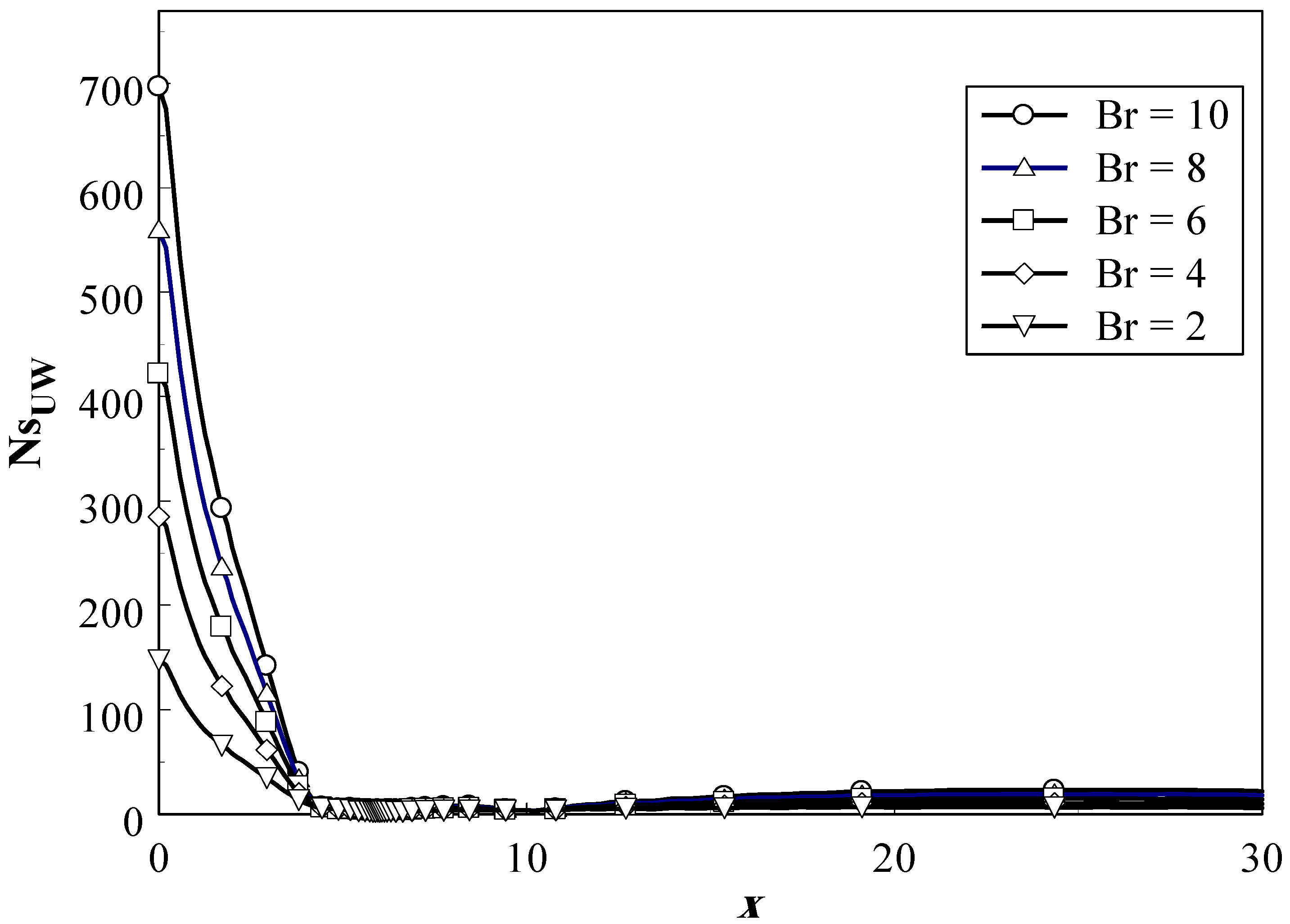
Fig. 12.
x-component velocity contour plots for Re = 800, 0<x<12.
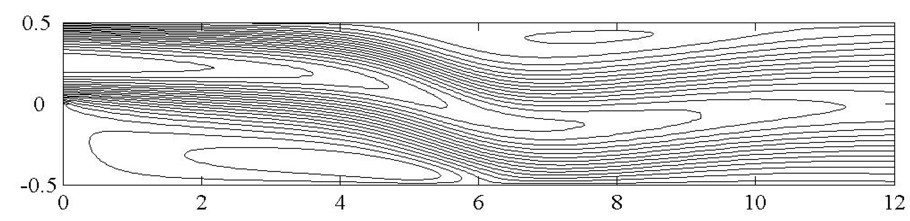
Fig. 13.
Nusselt number distribution along the top and bottom walls.

Fig. 14.
Variation of Ns with Re for different values of Br for τ=2
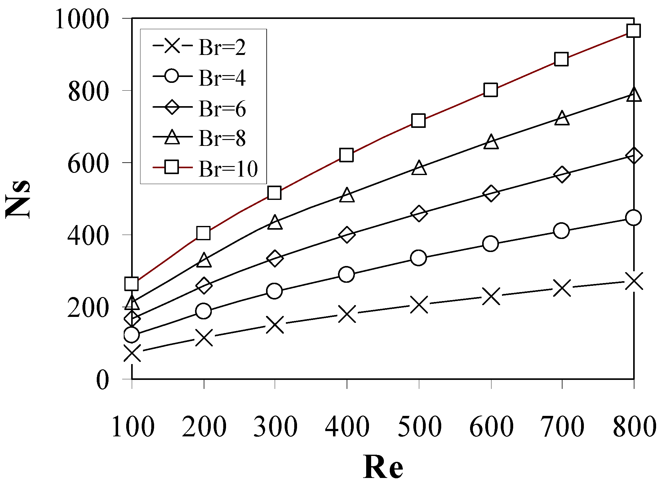
Fig. 15.
Variation of Ns with Re for different values of τ, Br = 1.


| Grid Size | Xr | X2 | X3 | Nusselt number |
| 13×24 | 6.50 | Not predicted | Not predicted | 8.50 |
| 25×50 | 4.00 | 2.50 | 5.20 | 8.40 |
| 37×75 | 3.35 | 2.35 | 5.47 | 8.38 |
| 49×100 | 5.77 | 4.65 | 9.45 | 8.30 |
| 75×150 | 5.90 | 4.81 | 9.76 | 8.25 |
| 101×199 | 6.00 | 4.81 | 10.10 | 8.24 |
| 125×250 | 6.03 | 4.81 | 10.14 | 8.236 |
| 151×299 | 6.03 | 4.81 | 10.15 | 8.234 |
| Authors | Type of Work | Xr | X2 | X3 |
| Armaly et al. [10] | Experimental | 7.20 | 5.30 | 9.40 |
| Vradis et al. [15] | Numerical | 6.13 | 4.95 | 8.82 |
| Kim and Moin [13] | Numerical | 6.00 | No data | No data |
| Gartling [12] | Numerical | 6.10 | 4.85 | 10.48 |
| Pepper et al. [16] | Numerical | 5.88 | 4.75 | 9.80 |
| Present Work | Numerical | 6.03 | 4.81 | 10.15 |
© 2005 by MDPI (http://www.mdpi.org). Reproduction for noncommercial purposes permitted.
Share and Cite
MDPI and ACS Style
Abu-Nada, E. Numerical Prediction of Entropy Generation in Separated Flows. Entropy 2005, 7, 234-252. https://doi.org/10.3390/e7040234
AMA Style
Abu-Nada E. Numerical Prediction of Entropy Generation in Separated Flows. Entropy. 2005; 7(4):234-252. https://doi.org/10.3390/e7040234
Chicago/Turabian StyleAbu-Nada, Eiyad. 2005. "Numerical Prediction of Entropy Generation in Separated Flows" Entropy 7, no. 4: 234-252. https://doi.org/10.3390/e7040234