On a simple derivation of a family of nonextensive entropies from information content

Abstract

The nonextensive entropy of Tsallis can be seen as a consequence of postulates on a self-information, i.e., the constant ratio of the first derivative of a self-information per unit probability to the curvature (second variation) of it. This constancy holds if we regard the probability distribution as the gradient of a self-information. Considering the form of the nth derivative of a self- information with keeping this constant ratio, we arrive at the general class of nonextensive entropies. Some properties on the series of entropies constructed by this picture are investigated.

1 Introduction

Tsallis statistics[1] can be seen as a formalism based on a pair of deformed functions of usual exponential and logarithmic ones[2,3]. Their deformed functions are called the q-exponential and the q-logarithmic functions, respectively. The q-exponential function is defined as $e_q^x={\left[1+\left(1-q\right)x\right]}_{+}^{1/1-q}$, where [x]₊ = max{x, 0} and the q-logarithmic function ln_qx = (x^1−q − 1)/(1 − q), where x ≥ 0. The derivation of the deformed (or, the generalized) form of the usual logarithmic entropy and its mathematical structure based on it have been attracted much attention. Furthermore, studies on deriving probability distribution functions consistent with these generalized entropies from microscopic dynamics have been done [4,5] and some statistical mechanical foundations of the Tsallis distribution are summarized in Ref.[6] (and references therein). One question arises regarding the origin of the nonextensive entropy and the clarification of it is desirable for further study. Although the Tsallis entropy was devised in physics in a heuristic way motivated by multi- fractals[1], the use of it has been stretched to neighboring scientific fields such as information theory [7], econophysics[8], to name a few. Therefore, it is required to understand how the entropy is connected to the existing quantities. In this paper, we shall provide a partial answer to that query from the information theoretical point of view and present a general form of entropies.

Let us review the elicitation procedure of the Tsallis entropy. It is shown that the Tsallis entropy is derived from the following set of postulates and a notation on the self-information with standard average:

Postulate 1: For p ∈ [0, 1], h(p) is a continuous function

Postulate 2: For two different probabilities p₁ and p₂, h(p₁p₂) = h(p₁)+ h(p₂)+ λh(p₁)h(p₂), where λ ≠ 0

Postulate 3 (Notation): h(0) = 1/(q − 1), where q ∈ ℝ.

Since λ ≠ 0, the expression in Postulate 2 can be rewritten as a factorized form s(p₁p₂) = s(p₁)s(p₂) with s(p) = 1 + λh(p). The trivial solution s(p) = 0, which gives constant function for h(p) (= −1/λ) is not appropriate due to the fact that it provides constant information irrespective of the associated probabilities. Therefore we may put the general solution as s(p) = p^q−1[9], which leads to the form h(p) = (p^q−1 − 1)/λ. From Notation, we determine λ = 1 − q, hence the linear average of h(p) (i.e., ∑_kp_kh(p_k)) leads to the Tsallis entropy. Since Notation fixes the value of λ, if we replace Notation with h(1/2) = 1, resulting entropy gives the type β generalization of Shannon entropy by Havrda-Charvat[10] and Daroczy[11]. In this case the factor λ becomes 2^1−β − 1, where β ≠ 1. The difference between the Tsallis entropy and the type β entropy stems from the arbitrary factor which fixes the form of the self-information. It should be noted that, in a nonadditive self-information h(p) = (p^q−1− 1)/(1 − q), we have finite information for q ≠ 1 even if the least probable event occurs[7], whereas we get infinite information in the ordinary logarithmic definition of the self-information (see Appendix for the definition).

In view of the fact that some alternative entropies and discussions based on them are recently attracting much attention for their potential uses and applications[12,13,14], our motivation in this study is set to the investigation for certain types of a hierarchical structure embedded in the generalized entropies starting with a self-information, which characterizes the associated en- tropy. This paper presents a procedure for obtaining a series of generalized class of (nonextensive) entropies, which include some existing entropies as special cases.

In the next section, we give an elementary prescription in order to obtain a series of nonextensive entropies including Tsallis one. In Section 3, we brieffy discuss properties of basic ingredients for the nonextensive entropies. We present our conclusions in the last section.

2 A method to construct a generalized class of entropies

Information content is a basic quantity for measuring information of systems considered in in-formation theory. This notion is used for making entropies in our study. As a starting point, let us consider a probability distribution under α rescaling transformation defined on ℝ, where α (α ≠ 1) is a positive real number. The transformed probability distribution p_α(x) is defined as p_α(x) = αp(x/α). In general, the value of α determines the broadness and the size of the distribu-tion. When α < 1, p_α(x) shrinks, whereas if α > 1 it enlarges, however, its shape is maintained. In our present consideration, we focus on a special case with respect to this rescaling, where the probability function is invariant under the transformation:

$$\alpha p\left(\frac{x}{\alpha }\right)=p\left(x\right)$$

(1)

This transformation expresses that the probability distribution is a homogeneous function of degree one. It can be shown that, when the probability distribution is continuous on [0, 1], the ratio p(x)/x is found to be constant over this range. For positive integers n_i (i = 1, … , 4) satisfying n₁/n₂(= r₁), n₃/n₄(= r₂) ∈ [0, 1], repeated use of the equation (1) yields

$$\begin{array}{ccc}\hfill p\left(n_1/n_2\right)& =& n_{1}p\left(1/n_1·n_1/n_2\right)=n_{1}p\left(1/n_2\right)\hfill \\ & =& n_1{n}_{4}p\left(1/n_2·1/n_4\right)=n_1{n}_{4}p\left({\left(n_2{n}_3\right)}^{-1}·\left(n_3/n_4\right)\right)\hfill \\ & =& n_1/n_2·n_4/n_{3}p(n_3/n_4),\hfill \end{array}$$

(2)

which leads to p(r₁)/r₁ = p(r₂)/r₂. Therefore, the ratio p(x)/x results in a constant value. This fact constitutes a crucial basis in the following consideration. It is shown that the constant ratio of the change of the self-information per unit probability to its curvature (second derivative) leads to the Tsallis entropy. For this purpose, we add the following postulate:

Postulate 4: The ratio $\frac{h\prime \left(x\right)/x}{h\prime \prime \left(x\right)}$ is invariant under transformation Eq.(1).

This postulate implies (h’(x)/x)/h’’(x) = const., in which the general solution can be expressed as h’(x) = ax^b (a,b ∈ ℝ). Then, if we choose a = −1, b = q − 2, and setting the integration constant as 1/(q − 1), we obtain the form h(x) = ln_q(x⁻¹). This form leads to the Tsallis entropy if we use the standard mean value ∫xh(x)dx (If we employ the escort average[15], we have the normalized Tsallis entropy[7,16,17]). We immediately generalize the above procedure to the nth derivative of the self-information. That is,

Postulate 4’: The ratio $\frac{h^{\left(n\right)}\left(x\right)/x}{h^{\left(n+1\right)}\left(x\right)}$ is invariant under transformation Eq.(1), where h(x) is a Cⁿ⁺¹ class function.

The general solution of the above expression can be put as h⁽ⁿ⁾(x) = ax^q−(n+1) + b. Therefore, we obtain the solutions:

$$h\left(x\right)=\{\begin{array}{c}{\displaystyle \sum _{k=1}^{n+1}{c}_{k-1}\frac{x^{k-1}}{\left(k-1\right)!},c_n=a+b\left(\text{if} q=n+1\right)}\\ \frac{a{x}^{q-1}}{C\left(q;n\right)}+{\displaystyle \sum _{k=1}^{n+1}{c}_{k-1}\frac{x^{k-1}}{\left(k-1\right)!},c_n=b\left(\text{if} q\ne n+1 \text{and} q\ne n\right)}\\ \frac{a{x}^{n-1}}{\left(n-1\right)!}\text{ln}x+{\displaystyle \sum _{k=1}^{n+1}{c}_{k-1}\frac{x^{k-1}}{\left(k-1\right)!},c_n=b\left(\text{if} q=n\right)}\end{array},$$

(3)

where C(q; n) = (q − 1)(q − 2) (q − n) and c₀,...,c_n are integration constants. We find that the Shannon entropy (the self-information by Hartley[18]) is recovered when n = 1, a = −1, b = 1 and c_k = 0, ∀k in the third line of the above expression. Since the form of the cases q ≠ n + 1 and q ≠ n in the second line can be considered as a generic self-information, we shall consider properties of it in the next section. The values of a and c_k’s are constrained by the feature of h(x) in addition to the sign of C(q; n). Using the standard definition of the mean value, the resulting average of the self-information (i.e., entropy) can be expressed as follows:

$$\frac{a}{C\left(q;n\right)}{\displaystyle \sum _i{p}_i^q}+{\displaystyle \sum _i{\displaystyle \sum _{k=1}^{n+1}{c}_{k-1}\frac{p_i^k}{\left(k-1\right)!}}, \left(n\ge 1\right)}.$$

(4)

We denote this entropy as $H_q^n$(p; {c_k}), where a set of probabilities is denoted simply by p. Some existing entropies can be expressed as a paticular class of $H_q^n$(p; {c_k}):

when a = −1,

(1)

the Rényi entropy of order α, ln${\displaystyle {\sum }_i{p}_i^{\alpha }}/\left(1-\alpha \right)$ is expressed as $\ln \left[\left(1-\alpha \right)H_{\alpha }^1\left(p;0,0\right)\right]/\left(1-\alpha \right)$.

(2)

$H_q^1\left(p;\frac{1}{q-1},0\right)$ is equivalent to the Tsallis entropy $\frac{{\displaystyle {\sum }_i{p}_i^q-1}}{1-q}$.

(3)

the quadratic information, $1-{\displaystyle {\sum }_i{p}_i^2}$ (e.g.,[19]) is given by $H_2^1$(p; 1, 0).

(4)

the type β entropy is $H_{\beta }^1\left(P;\frac{1}{1-2^{1-\beta }},0\right)$.

If we allow a to take various values, we can express other entropies with $H_q^n$(p; {c_k}). For example, the cubic information $1-{\displaystyle {\sum }_i{p}_i^3}$ [20] can be represented either by $H_3^2$ (p; 1, 0, 1) with a = −1, or $H_3^2$ (p; 1, 0, −2) with a = 0, or $H_3^1$ (p; 1, 0, 0) with a = −2.

In the subsequent discussion, we set a = −1 by taking into account that the conventional entropy is recovered in this case. If we put a = −k_B, where k_B is the Boltzmann factor, it can be regarded as an entropy in statistical mechanics, however, recall that we usually put k_B = 1 to make the entropy dimensionless.

3 Some general properties of $H_q^n\left(p;\left\{c_k\right\}\right)$

There are many properties characterizing an entropy. Among these, we shall investigate ingre-dients to clarify the relation to the physical entropy, which is expected to have concavity[21] for instance. Our way of consideration is to determine or to give constraints between parameters included in $H_q^n\left(p;\left\{c_k\right\}\right)$ so that the generalized entropies can possess the fundamental features below.

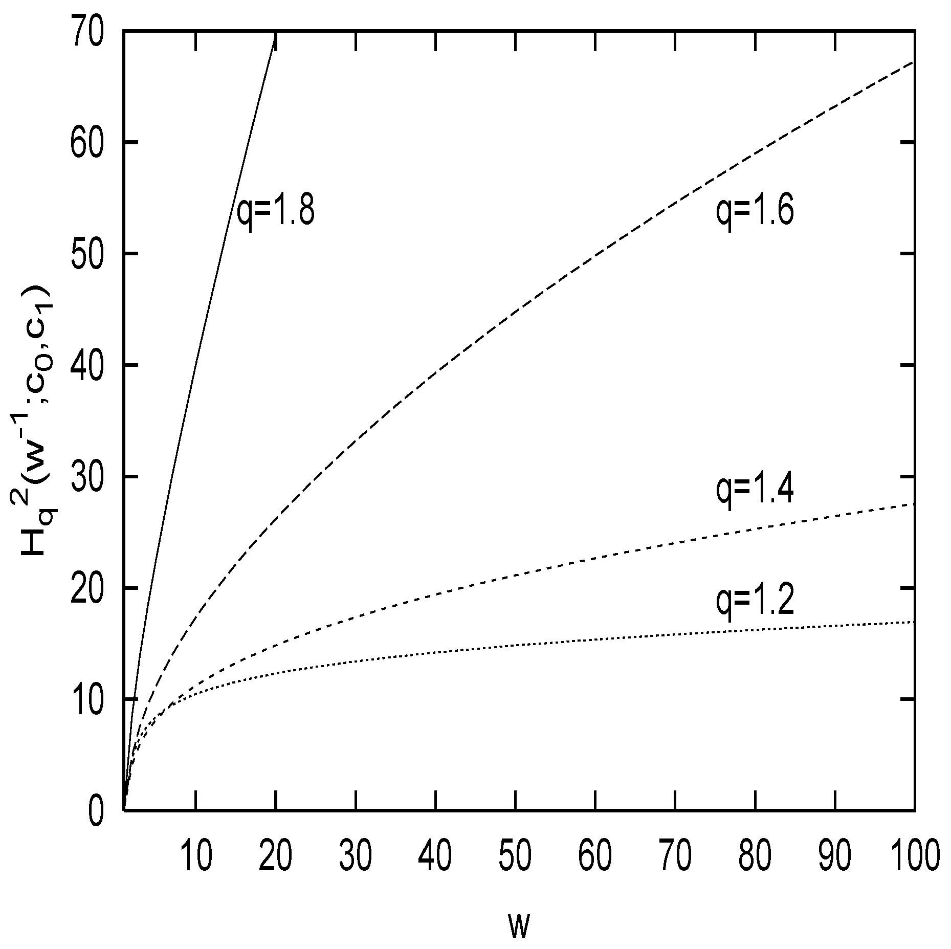
Certainty and monotonicity w.r.t the number of states:

In order to guarantee the certainty $H_q^n\left(1,0,\dots ,0;\left\{c_k\right\}\right)=0$, we need to have the relation $C{\left(q;n\right)}^{-1}={\displaystyle \sum _{k=1}^{n+1}{c}_{k-1}/\left(k-1\right)!\left(a=-1\right)}$. This provides a strong constraint on the value of c_k’s and q for a given order n. Whether or not the entropy for the equiprobability p_i = w⁻¹ is an increasing function of w, in general, depends complicately on the range of value q and the values of c_k’s. As a specific example, let us mention the case n = 1. The behavior of $H_q^1\left(w^{-1};c_0;c_1\right)$ is shown in Figure 1, where the relation that ensures the certainty condition described above has used. It increases monotonically with respect to w when 1 < q < 2 for all values of c₀. For other regions of q, $H_q^1\left(w^{-1};c_0;c_1\right)$ monotonically decreases as w grows. In a specific choice of the integration constants, i.e., when c_k = 1, ∀k, $d{H}_q^n\left(w^{-1};1,\dots ,1\right)/dw$ is written as $-w^{1-q}/C\left(q;n\right)+{\displaystyle {\sum }_{i=1}^n{w}^k/k!}$ (a = −1) for q ≠ n. This means that $H_q^n\left(w^{-1};1,\dots ,1\right)$ can be an increasing function of w (when the values of n and q are chosen appropriately), which is one of the desirable behavior for an entropy at the equiprobability.

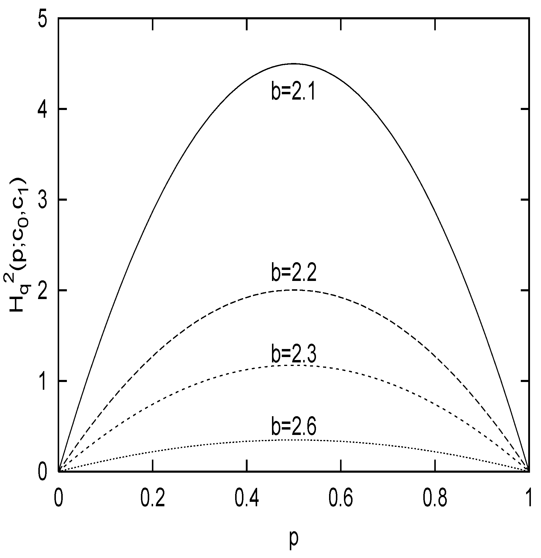
Two-state system:

One of the simple examinations of a behavior of the generalized entropy is for a two-state sys-tem (W = 2), where the probabilities is defined p₁ = p and p₂ = 1 − p, respectively. From the definition, straightforward calculations yield a final expression:

$$H_q^1\left(p;c_0,c_1\right)=\frac{1-p^q-{\left(1-p\right)}^q}{\left(q-1\right)\left(q-2\right)}+2c_{1}p\left(p-1\right),$$

(5)

where we set a = −1, and used the end-points condition (i.e, the entropy should vanish at p = 0 and p = 1, leading to the relation c₀ + c₁ = [(q− 1)(q − 2)]⁻¹). Figure 2. shows the shape of $H_q^2\left(p;c_0,c_1\right)$ for different values of q, where the end-points condition and the concavity are both satisfied. Note that the concavity of the entropy holds only for the parameter range $c_1<\frac{q}{q-1}{2}^{1-q}$.

Expansibility:

$H_q^n\left(p;\left\{c_k\right\}\right)$ is expansible for all q and n, i.e.,

$$H_q^n\left(p_1,\cdots ,p_w;\left\{c_k\right\}\right)=H_q^n\left(p_1,\cdots ,p_w,0;\left\{c_k\right\}\right),$$

(6)

where w denotes the number of states. Regarding the entropy for uniform probabilities and certainty, we shall add comments in the next section.

Transformation from discrete entropy to continuous one:

If we define a discrete probability as p_i = p($\stackrel{-}{x_i}$)∆x (∀i, i = 1,... , m), where $\stackrel{-}{x_i}$ ∈[x_i−1, x_i] and the bins of length ∆x = x_i − x_i−1 with x₀ and x_m being end-points of its support, and p(x) is continuous within the bins, then the corresponding discrete entropy can be expressed as

$$p_q^n\left(p;\left\{c_k\right\}\right)=-{\displaystyle \sum _{i=1}^m\frac{\Delta x{p}^q\left(\stackrel{-}{x_i}\right)}{C\left(q;n\right)}}{\left(\Delta x\right)}^{q-1}+{\displaystyle \sum _{i=1}^m{\displaystyle \sum _{k=1}^{n+1}\frac{c_k-1}{\left(k-1\right)!}}}\Delta x{p}^k\left(\stackrel{-}{x_i}\right){\left(\Delta x\right)}^{k-1}.$$

(7)

If we put ∆x = 1 as explained in Ref.[22], the first and second terms come close to the integral of $-p^q\left(\stackrel{-}{x_i}\right)/C\left(q;n\right)$ and ${\displaystyle {\sum }_{k=1}^{n+1}{c}_{k-1}}{p}^k\left(\stackrel{-}{x_i}\right)/\left(k-1\right)!$, respectively by the Riemann integrability.

4 Concluding remarks

It is noteworthy that for the general form of entropy such as ${\displaystyle {\sum }_{i}f\left(p_i\right)}$ (in our case f(p_i) = p_ih(p_i)), the additivity of the entropy holds only when it satisfies the relation [p_if’’(p_i)’ = 0. This relation straightforwardly leads to the Shannon form f(p_i) = −p_iln p_i [23]. In this sense, a family of generalized entropies constructed in this paper can be considered to be intrinsically nonadditive.

Since the generalized form of entropy presented in this study contains a number of parame-ters (integration constants) depending on the order n, some properties satisfied by some known generalized entropies can be used as constraints for the parameters. Among preferable properties that should be possessed by entropies, a behavior for the equiprobability and certainty have been mentioned. As for obtaining the analytical expression of the equilibrium distribution p_i by the Lagrange multiplier method, it seems to be diffcult to perform it for the general form. This is mainly because of the fact that the constrained (by energies) entropy functional, which should be solved, becomes a polynomial with respect to p_i.

In this paper, we have presented an elementary procedure to obtain a series of nonexten-sive entropies from some postulates on the self-information. As a main ingredient, the ratio (h⁽ⁿ⁾(x)/x)/h⁽ⁿ⁺¹⁾(x) has been assumed to be constant. Our formulation provides us that the Tsallis nonextensive entropy can be viewed as a special realization of a set of the large class of generalized entropies. In fact, this view is not new perspective. Some authors seem to have been shared this viewpoint in developing the generalized entropies[14,24,25]. We believe that the discussion presented in this study serves as understanding the structure of entropies and giving a deeper insight into a number of (generalized) entropies, not from a heuristic definition. We note that applications of these entropies to systems both in statistical mechanics and in information theory are potentially fruitful, but we need to know what aspect of the system relatetes to the nonextensivity parameters for further studies.