
Performance of Bearing Ball Defect Classification Based on the Fusion of Selected Statistical Features

1
Ecole Nationale Supérieure d’Ingénieurs de Tunis (ENSIT), University of Tunis, Tunis 1007, Tunisia
2
The Matériaux, Mesures et Applications (MMA) Laboratory, University of Carthage, Carthage 1054, Tunisia
3
Laboratoire des Signaux et Systèmes, CNRS, CentraleSupelec, Université Paris Saclay, 91192 Gif sur Yvette, France
4
Group of Electrical Engineering of Paris, CNRS, CentraleSupelec, Université Paris Saclay, 91192 Gif sur Yvette, France
*
Author to whom correspondence should be addressed.
Entropy 2022, 24(9), 1251; https://doi.org/10.3390/e24091251
Submission received: 30 June 2022
/
Revised: 19 August 2022
/
Accepted: 31 August 2022
/
Published: 5 September 2022
(This article belongs to the Special Issue Fault Diagnosis Methods Based on Information Theory or Machine Learning: From Theory to Application)
Abstract
:Among the existing bearing faults, ball ones are known to be the most difficult to detect and classify. In this work, we propose a diagnosis methodology for these incipient faults’ classification using time series of vibration signals and their decomposition. Firstly, the vibration signals were decomposed using empirical mode decomposition (EMD). Time series of intrinsic mode functions (IMFs) were then obtained. Through analysing the energy content and the components’ sensitivity to the operating point variation, only the most relevant IMFs were retained. Secondly, a statistical analysis based on statistical moments and the Kullback–Leibler divergence (KLD) was computed allowing the extraction of the most relevant and sensitive features for the fault information. Thirdly, these features were used as inputs for the statistical clustering techniques to perform the classification. In the framework of this paper, the efficiency of several family of techniques were investigated and compared including linear, kernel-based nonlinear, systematic deterministic tree-based, and probabilistic techniques. The methodology’s performance was evaluated through the training accuracy rate (TrA), testing accuracy rate (TsA), training time (Trt) and testing time (Tst). The diagnosis methodology has been applied to the Case Western Reserve University (CWRU) dataset. Using our proposed method, the initial EMD decomposition into eighteen IMFs was reduced to four and the most relevant features identified via the IMFs’ variance and the KLD were extracted. Classification results showed that the linear classifiers were inefficient, and that kernel or data-mining classifiers achieved classification rates through the feature fusion. For comparison purposes, our proposed method demonstrated a certain superiority over the multiscale permutation entropy. Finally, the results also showed that the training and testing times for all the classifiers were lower than 2 s, and 0.2 s, respectively, and thus compatible with real-time applications.
1. Introduction
Electric actuators are increasingly present in several application areas such as transport, health or renewable energy. At the same time, the requirements for operational safety and energy efficiency are becoming increasingly stringent. In response, condition-based maintenance was introduced. It requires regular monitoring of all system components, including electrical machines. Electrical machines operating increasingly under severe conditions or at the limits of their capacity are subject to faults that can lead to failures [1,2,3]. Investigations in several industrial fields have revealed that rolling bearing elements (RBEs) are the main sources of failures for almost to of low- to high-power machines [4,5]. Several studies [6,7] have concluded that bearing ball fault is the most difficult to diagnose (detection and classification) because its effects are strongly attenuated by the mechanical structure.
Bearing balls can be affected by corrosion, spalling, high temperatures or premature wear due to overloading. In the long term, these degradations lead to holes in the balls.
It is of a paramount importance to investigate these types of faults considered as incipient ones and that can be found in such electrical machines (synchronous or asynchronous machines). In the considered testbed, three bearings were degraded. For each of them, a hole with a different diameter was drilled in a ball to evaluate the proposed diagnostic method.
It is usual to consider that fault detection and diagnosis methodologies can be summarised in four major steps: (1) modelling, (2) data preprocessing, (3) feature extraction and selection and (4) feature analysis for decision-making. The modelling is derived from physics-based models or historic data. Because accurate analytical models are not readily available, a data-driven approach has become more and more attractive thanks to the increasingly digitalised systems. Vibration signals are still considered to contain the most relevant information about the health of the bearings [8,9,10,11]. In fact, the main advantages of vibration-based diagnosis is its ability to detect different types of defects, either distributed or localised [9].
Before the extraction and analysis of the most representative fault features, raw time-series vibration signals need to be preprocessed [8,12,13]. In this step, several operations can be done depending on the fault detection requirements, the quantity of data and the signal properties. One of the main operation consists in selecting the most appropriate space of representation: time domain, frequency domain, or time–frequency domain [14]. The varying operating conditions lead to transient and nonstationary signals [15,16]. Therefore, time-domain features and classical frequency-domain techniques such as FFT fail to diagnose bearing faults. Over the years, several time–frequency (and time–scale) techniques such as the short-time Fourier transform (STFT) [17,18], wavelet transform (WT) and its derivatives namely the Wavelet packet transform (WPT), discrete wavelet transform (DWT) [19,20], and Hilbert–Huang transform (HHT) [21,22] have been used to address this issue. Nonetheless, the STFT suffers from a fixed window length, while the performance of the WT strongly depends on the selection of the mother wavelet and the decomposition level. Moreover, both methods are limited by the two contradictory targets that cannot be reached simultaneously: a high time and frequency resolution [23].
In the past few decades, other decomposition techniques have been applied to vibration time series [24,25], among them, the empirical mode decomposition (EMD) [26,27], ensemble empirical mode decomposition (EEEMD) [28,29,30] or variational mode decomposition (VMD) [31,32,33]. Despite its shortcomings such as mode mixing and end effects [27,34,35], the EMD is still very popular. In fact, EMD decomposes a time-series signal into a finite number of signals denoted as intrinsic mode functions (IMF), and a residue. Each IMF represents the original signal in a frequency band ranging from high to low frequencies. Compared to the original signal, the IMFs can better describe the intrinsic properties of the raw data [36]. However, the fault information is not evenly distributed among the IMFs.
Therefore, it is of utmost importance to select the most relevant IMFs and consider the best features in order to obtain the highest detection and classification rates. Moreover, the retained IMFs should also be robust to nuisances (environmental noise) and variable operating conditions. In the literature, most of the studies focus on the classification between inner race, outer race, cage and ball faults [11,12]. However, the classification of ball faults based on their severities is more tedious and still an open research topic. This paper addresses this problem and highlights the performance according to the chosen family of classification techniques. Indeed, if we consider that when using statistical clustering techniques, several solutions can be considered according to the nature of the data, their linearity, their separability, and so forth, then the techniques can be separated in different families. With no loss of generality, we can mention: linear projection techniques such as the principal component analysis [37] (PCA); kernel-based nonlinear techniques such as the kernel principal component analysis (KPCA), support vector machines (SVMs) [38]; kernel estimation techniques such as the K-nearest neighbours (KNN) algorithm [39]; tree-based techniques such as decision trees (DTs) [40]; or probabilistic techniques such as the naive Bayes (NB) classifier [41]. For the ball bearing classification problem, we propose to evaluate and compare the efficiency of these techniques.
To the best of our knowledge, a piece of equipment using vibration signal analysis for industrial applications provides general information (fault isolation and a rough estimate of the severity of the defect) on mechanical defects: loosening, rotor unbalance, bearings or misalignment. The most usual professional bearing condition monitoring systems are based on the characteristics of specific harmonics (RMS, frequency) extracted from time series of vibration signals. However, the results could be biased due to ageing, variable load conditions and environmental nuisances. The proposed method detailed in this work complements the available instruments since it allows a more accurate analysis of bearing defects, in this case, balls. The proposed methodology allows a more accurate diagnosis up to the classification with information extracted from vibration data, which is so far the most popular in the industry. Thanks to the preprocessing, the proposed method extracts fault characteristics (statistical and distance-based features) that are the most sensitive to the defect and robust to the nuisance and load variations. Processing times are also compatible with real-time application. The proposed method is also in line with the growing use of machine learning techniques.
The organisation of the paper is as follows: Section 2 highlights the paper contribution, Section 3 describes the proposed ball fault diagnosis methodology. The EMD and the basics of each data representation technique are shortly reviewed, and the extracted features are introduced. Section 4 is devoted to the experimental evaluation of the classifiers using the CWRU database. The conclusion and future research are presented in Section 5.
2. Paper Contribution
In the following, we propose a four-step methodology to perform ball fault classification with the combination of properly selected statistical features. The vibration signals used to illustrate the rational of the approach were obtained from the Case Western Reserve University database [42]. In the preprocessing step, the EMD was adopted to decompose the original signal into IMFs. Then, the most relevant ones were retained from the analysis of their signal-to-noise ratio and their invariance to the operating conditions. The fault features selected were derived from their first four statistical moments (i.e., mean, variance, skewness, kurtosis) and their probability density functions (PDF) using the Kullback–Leibler divergence [43,44,45]. The selection process identified the most relevant features as the IMFs’ variance and the KLD. For the fault classification, the selected features were merged then analysed with several techniques including the traditional PCA, KPCA, SVM, and data exploration solutions with deterministic (KNN and DT) and probabilistic (NB) approaches. The classification performance of all these techniques was evaluated and compared in terms of training accuracy rate (TrA), testing accuracy rate (TsA), training time (Trt) and testing time (Tst). The most suitable classification technique was then highlighted and compared to the literature’s main results for this particular incipient fault diagnosis.
3. The Fault Diagnosis Methodology
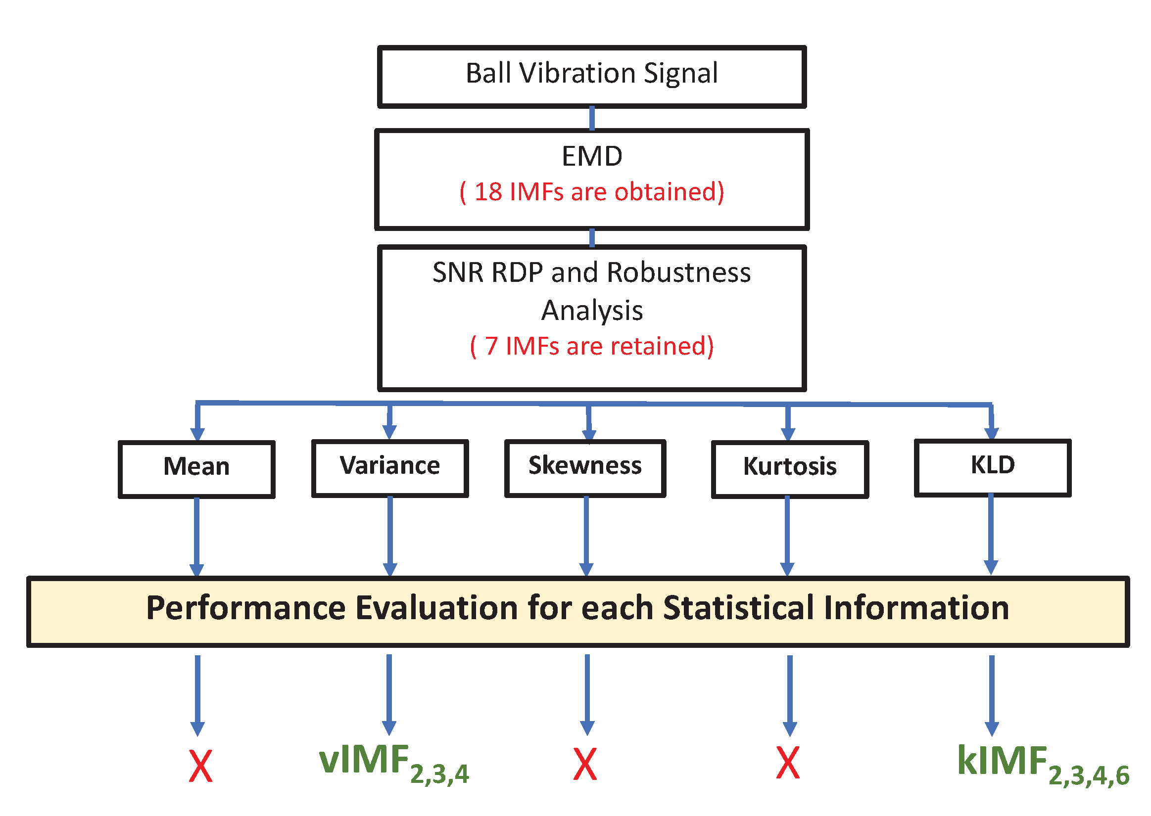
Figure 1 gives an overview of the methodology with the four steps.
3.1. Preprocessing and Feature Extraction and Selection
The first step, modelling, assumed the use of vibration raw data. With no loss of generality, the raw data used here were vibration time- dependent information recorded with a sampling frequency of 12 kHz using accelerometers located at 12 o’clock on the housing of the drive end and the fan end. This is detailed in Section 4.1, which describes the experimental data. Note that the data corresponded to the healthy and three faulty cases (0.007, 0.014, 0.021 inch) with four different load conditions: no load (L0), half-load (L1), full load (L2), overload (L3). These load conditions allowed us to clearly observe the influence of the machine’s torque.
For the second step, preprocessing, the raw vibration signals were decomposed into intrinsic mode functions (IMFs) using the EMD. In order to retain the most relevant IMFs [34] from the 18 IMFs, the relative deviation percentage (RDP) of the IMFs’ signal-to-noise ratio (SNR) was computed [46,47]. Table 1 presents the results.
IMFs with an SNR RDP greater than 40 dB were considered irrelevant as they were highly sensitive to the noise. As a consequence, only the first eight IMFs were considered for the bearing ball fault diagnosis. It was also proved in [47] that the first IMF () was very sensitive to the load variation. Finally, only to were retained for the feature extraction.
As depicted in Figure 2, in the feature extraction process, we analysed the first four statistical moments and the Kullback–Leibler divergence (KLD) of these seven IMFs for different operating conditions. It was found that [46,47]:
- The mean and the skewness had very poor detection performance
- The kurtosis had a very low sensitivity to the ball fault level.
Using the receiver operating characteristic (ROC) curve [48], the area under curve (AUC) was computed as an efficiency criterion to proceed with the feature selection. In Table 2, the AUC values are summarized for the four statistical moments, the KLD and each retained IMF. It can be noticed that the most relevant features are selected whatever the operating condition , , and .
It can be noticed that the KLD and variance for most of the IMFs are the main features to be retained whatever the operating condition. Furthermore, if the noise variation is considered, then the sensitivity of these features are kept for a reduced number of IMFs [46,47].
Finally, the most relevant features retained for the bearing ball extraction were as follows:
- Variance: , and ; denoted as
- KLD: , , and ; denoted as .
Note that the subscript j indicates the rank of the considered .
3.2. Feature Analysis
As shown in the flowchart from Figure 1, the choice of the appropriate classification technique depends on whether the data are linearly separable or not. In the following, a brief review of the classification methods proposed to be used in this work is presented.
3.2.1. Principal Component Analysis (PCA)
The PCA is a linear unsupervised technique. It projects the original data into a lower dimension subspace while minimising the reconstruction error [37]. This method has in fact received considerable attention in the fault detection and diagnosis framework over the last three decades since no prior complex physical knowledge on the process is needed. The only information required is a history of data representing several operating conditions.
However, most of the processes exhibit nonlinear behaviour and the measurements are affected with noise whose distribution may be unknown. Therefore, linear methods such as PCA may have poor performance. In the following, improved techniques are investigated such as:
- Kernel-based techniques: kernel principal component analysis (KPCA) and support vector machine (SVM);
- Deterministic systematic exploration techniques: K-nearest neighbours (KNN) and decision tree (DT);
- Probabilistic systematic exploration techniques: naive Bayes classifiers (NB).
3.2.2. Kernel Principal Component Analysis (KPCA)
KPCA was firstly proposed by Scholkop et al. [49] and was provided as an alternative to PCA, which allowed the nonlinear feature extraction from a dataset by using a specific kernel. As reported in the literature, this technique has been successfully used in fault detection and diagnosis (FDD) of several systems [50,51,52,53]. The main idea of this technique relies on mapping the data into a feature space through a nonlinear function (denoted as the kernel) so that PCA can be performed in that feature space. The kernel function is the core of the KPCA algorithm. It is a positive semidefinite function that introduces nonlinearity into the process. The most classic kernels considering two sample vectors x and y are:
- The polynomial kernel defined as ( is the kernel’s order):
- The Gaussian kernel defined as ( is the standard deviation of the kernel):
The performance of KPCA is strongly related to the selected kernel and to the tuning of its hyperparameters, which depends on the data distribution [38,54]. In the following, for each kernel, the performance is analysed with regard to the setting of each hyperparameter. Despite its advantages, KPCA is time- and memory-consuming as the size of the database increases with a third-order complexity , where N is the data set dimension and required storage capacity for an kernel matrix.
3.2.3. Support Vector Machine (SVM)
Used for classification, regression and outlier detection, an SVM is considered as one of the most attractive supervised machine learning algorithms and was developed by Vapnick in 1995 [55]. Its basic idea consists of finding the highest dimension feature space in which the projected data are linearly separable with the highest margin between the different classes. This projection also requires the selection and tuning of kernel functions. Therefore, choosing the kernel, then adjusting its hyperparameters, is also a critical task as it highly impacts the classification’s performance. As for KPCA, famous and widely used kernels are polynomial ones (i.e., Equation (1)) and Gaussian ones (i.e., Equation (2)). Their tuning are both considered for this study.
3.2.4. K-Nearest Neighbours (KNN)
KNN is a nonparametric, supervised, and easy to implement classification technique. This classifier is exclusively based on the selection of the classification metric, among which we can cite the Euclidean distance (Euc), the city block distance (CB), the Minkowsky distance (Mink) and the Chebyshev distance (Chb). The technique is based on distance estimation and the tuning of a predefined number of nearest neighbours denoted K [56]. In [57], the determination of K as well as the pertinent metrics were analysed. In the following, K was selected in the range of and Euclidean and city block distances were evaluated. They are recalled in the following.
If we consider two vectors A and B defined, respectively, with samples and such as and , the distance metrics are:
- Euclidean distance (Euc). It is defined by:
- City block distance (CB) given as:
3.2.5. Decision Tree (DT)
A DT is considered as one of the most popular supervised machine learning techniques for solving data classification or regression problems. With its graphical tree-based geometry, the decisions are positioned at the ends of the branches also called leaves [58,59,60]. As in the KNN algorithm, a DT is also based on two main parameters: the maximum split number criterion (MSpN), and the split criterion (Spc). In the following, MSpN was set to 50 to avoid overfitting. The maximum deviance reduction (MDR), twoing rule (TR) and Gini’s split criteria were adopted in our approach to tune the Spc. More details can be found in [57].
3.2.6. Naive Bayes (NB)
Naive Bayes is one of the powerful probability-based supervised machine learning classification method. It has been used in several applications due to its simple implementation, ease of physical interpretation, fast computation speed and excellent classification performance [61,62,63]. However, the assumption of conditional independence of variables may limit its performance when dealing with real vibration data.
4. Results and Discussions
In this section, first, we introduce the experimental testbed and the data. Then, we present the classification results for each of the method described in the previous section.
4.1. Experimental Data
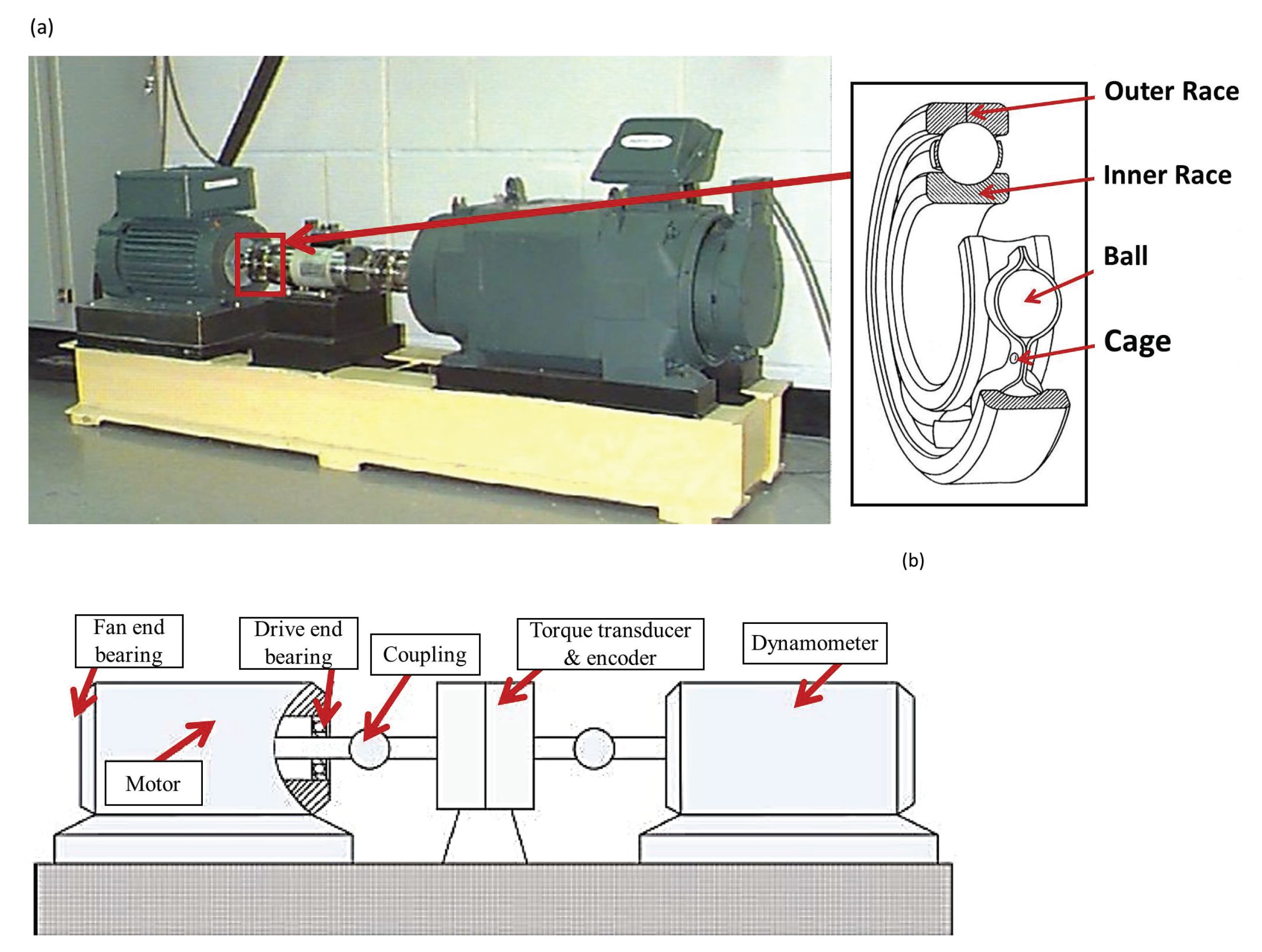
The dataset from the CWRU [42] was used to evaluate the proposed methodology. Figure 3 shows the CWRU’s experimental rig for the study of ball bearing defects. Vibration measurements were acquired with three accelerometers placed in the 12 o’clock position on the housing of the drive end (DE) and fan end (FE). SKF deep-groove ball bearings of 6205-2RS JEM and 6203-2RS JEM types were employed for both the DE end FE, respectively. Electro-discharge machining was used to generate different fault diameters ranging from to inch. Vibration signals were recorded at 12 kHz, under varying motor speeds from 1797 to 1720 rpm and four motor load operating conditions denoted as:
- No-load condition (): of the nominal load;
- Half-loaded condition (): of the nominal load;
- Fully loaded condition (): of the nominal load;
- Overloaded condition (): of the nominal load;
- Combination of all the load conditions: ().
The four classes under study were as follows:
- H: corresponding to the healthy behaviour (no fault);
- : faulty case with a severity of inch;
- : faulty case with a severity of inch;
- : faulty case with a severity of inch.
The training and testing time were evaluated using a computer operating with Windows 10 pro 64-bit and a processor Intel(R) Core(TM) i7-6500U CPU @ 2.50–2.59 GHz.
4.2. Experimental Validation
As depicted in Figure 2, in the first part of this work, the KLD of the retained IMFs were considered as input features for the classification stage. Under a single load condition, 900 realisations of this feature were computed for each feature and for each fault severity level. Taking the example of the unloaded condition with one fault severity, the input matrix for the classification was organized as follows:
Its elements can be generalized as to be the ith realisation of the KLD for the jth .
Therefore, for the fault cases (one healthy and three faulty cases), and the four load conditions, the data matrix size was (14,400 × 4. In the following, two-thirds of the data were used for training, and one-third for testing. Note that every case and condition were equivalently represented either in the training or the testing process.
4.2.1. Linear Classification with PCA
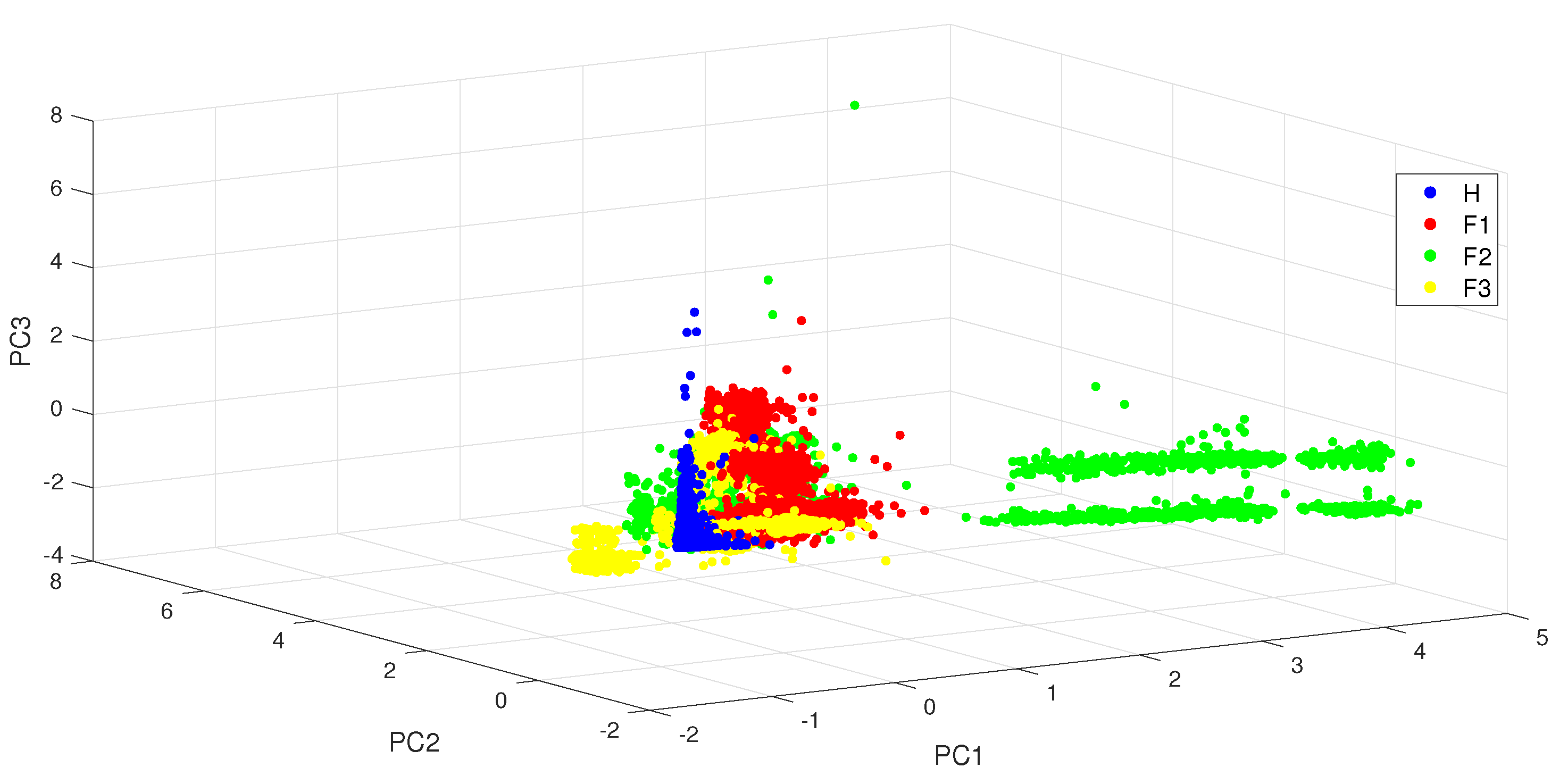
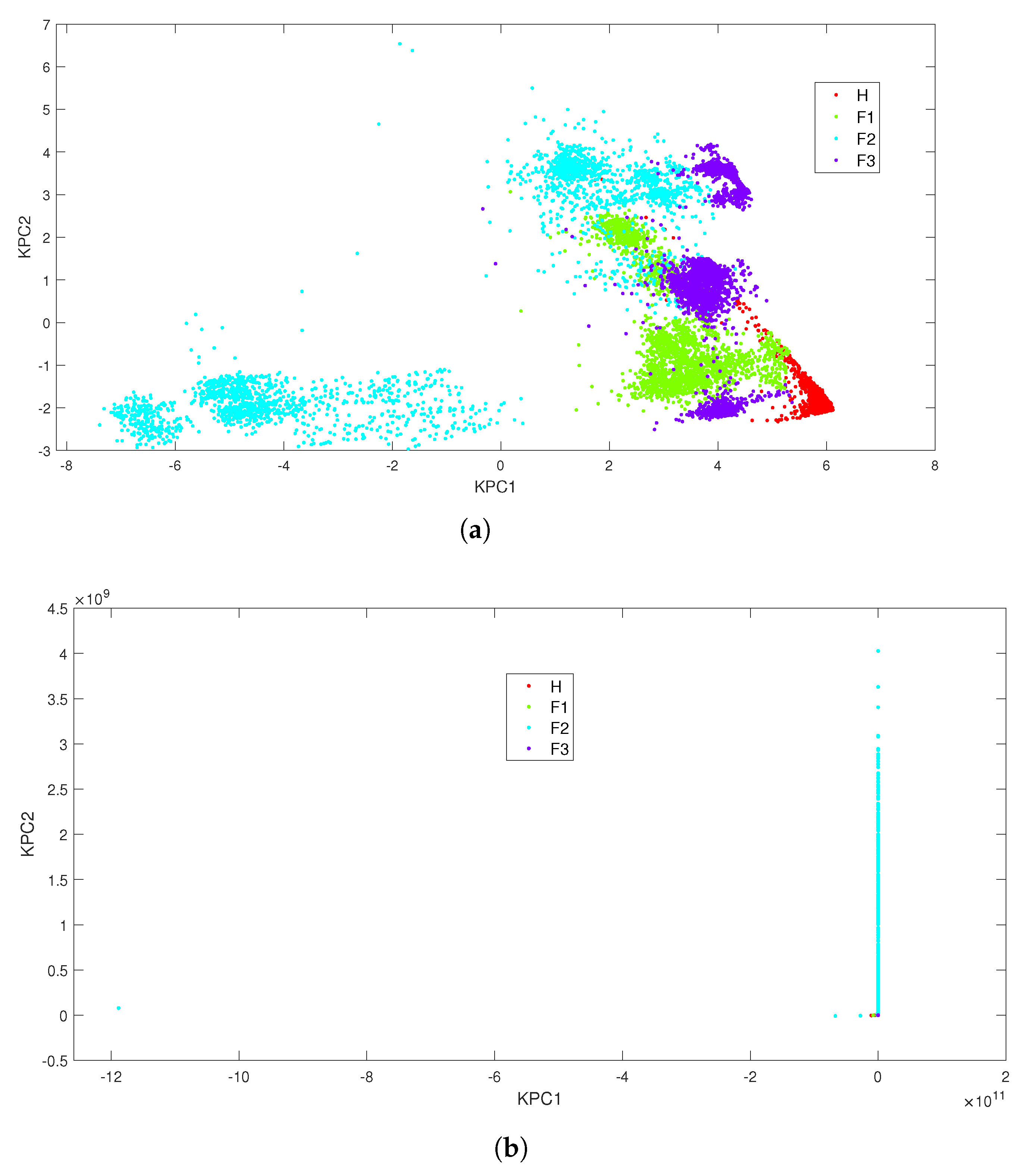
From the PCA contribution rates under different load conditions displayed in Table 3, it can be observed that more than of the information can be captured with the first three principal components. However, the projection of the data in the reduced dimension space shown in Figure 4 reveals a poor classification performance: the different classes have a huge number of overlaps.
In the following sections, nonlinear classifiers are evaluated.
4.2.2. Kernel-Based Classifiers
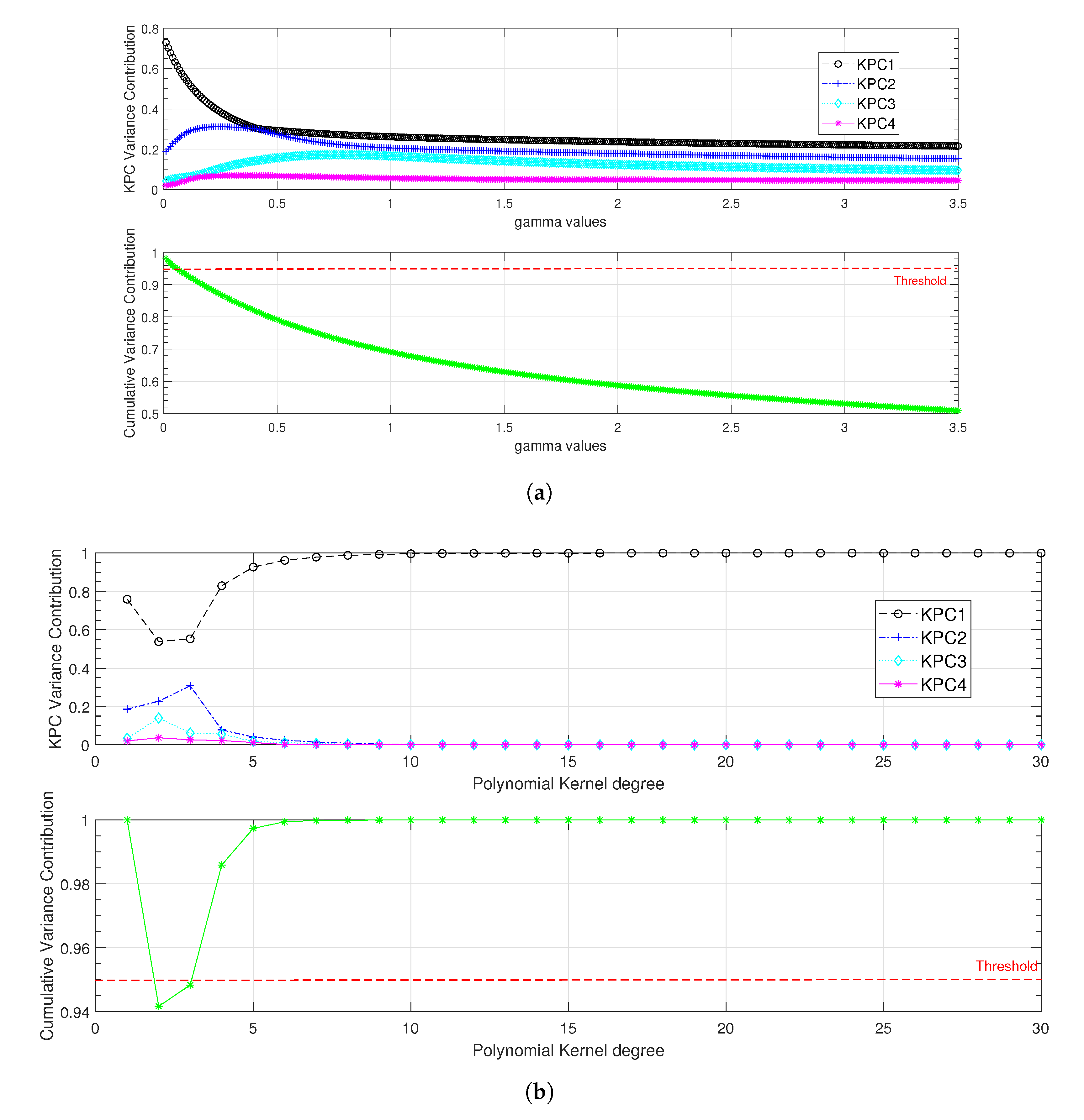
As mentioned in the previous section, the key point for this classifier is the selection and the tuning of the kernel. In the following, Gaussian and polynomial kernels were evaluated. For the Gaussian kernel, we proposed to vary from 0.01 to 3.5 with a step of 0.01. For the polynomial kernel, the degree p was varied between 1 and 30. The results under fully loaded condition are presented in Figure 5, where a threshold of for the cumulative variance contribution was used to set the most suitable values for each kernel’s parameters.
As shown in Figure 5, the most significant cumulative variance contribution was recorded for the Gaussian kernel with equal to , and for the polynomial kernel with an order . The degree of the polynomial kernel was set to 6 to minimise the computation time. Once the kernels had been tuned, they were evaluated with all load conditions. The results presented in Table 4 show that with the polynomial kernel, the first kernel principal component (KPC) is of great significance ( of the cumulative variance) while three KPCs are required to reach of the feature variation with the Gaussian kernel.
The data projection displayed in Figure 6 shows a poor performance of the classifier whatever the kernel is. A kernel-based technique with a higher dimensional projection space such as a SVM could be an option. However, in previous works [57,64], it was shown that a SVM combined with different approaches (one-against-all, one-against-one and directed acyclic graph SVM) could provide satisfactory classification results. However, these results were obtained to the detriment of high training times ( 132.1 s for the polynomial kernel and 14.05 s for the Gaussian one). Therefore, in the following, systematic data exploration techniques are evaluated: deterministic techniques such as KNN and DT and a probabilistic-based approach (NB).
4.2.3. Classification Results Based on the Systematic Data Exploration Strategy
In this study, deterministic (KNN, DT) and probabilistic (NB) classification techniques were evaluated and compared in terms of the following criteria: training accuracy rate , testing accuracy rate , training time and testing time .
Based on the results reported in Table 5, we can draw several conclusions when using only the KLD of the most sensitive :
- Under the single-load condition, all the three classifiers exhibited good performance despite a low testing accuracy rate of for the NB classifier;
- Under the combined-load condition, the performance of the NB classifier was severely degraded with and for the training accuracy rate and the testing accuracy rate, respectively.
To improve the classification results, we propose in the following to merge the most relevant features (variance and KLD of and ) as displayed in Table 6.
Three different case studies were considered:
- ■
- Case study with four features
- □
- KLD and variance of and , denoted as ;
In this case study, the KLD and the variance of the selected IMFs ( and ) were merged together for each load condition as in the following matrix.where and denote the KLD and variance of the jth component for their ith realisation, respectively. - ■
- Case study with two features
- □
- KLD and variance of , denoted as ;
- □
- KLD and variance of , denoted as ;
- □
- Variances of and , denoted as ;
- □
- KLD of and , denoted as .
- ■
- Case study with one feature
- □
- Variance of , denoted as ;
- □
- Variance of , denoted as ;
- □
- KLD of , denoted as ;
- □
- KLD of , denoted as .
Note that for all the case studies, a well balanced two-thirds of the data were used for training, and one-third for testing as mentioned before.
In a first stage, we present the results of the classification when the four features are merged. These results are displayed in Table 7. Compared to those obtained in Table 5, where only the were used, we can notice that the NB’ results are far better. For example, the testing accuracy rate significantly increased from to under . The training and testing accuracy rates were almost for KNN and DT under all load conditions. Compared to the previous case study where only the KLD was used, the classification performance was far better when the KLD and variance of the retained were merged. For the training time and testing time criteria, the variations for all the classifiers were not too significant.
These results are encouraging for bearing ball fault classification using the CWRU Database. In fact, Li et al. in [6], provided a comprehensive benchmark study of the CWRU Database with several entropy-based fault classification methods. They pointed out the difficulty of dealing with bearing ball fault, particularly in the case of (the 0.014-inch fault severity) where most of the classification algorithms exhibited a low performance. In Table 8, we present the comparison results between the multiscale permutation entropy (MPE), highlighted in [6], and our proposed method based on KLD and variance for the specifically selected IMFs.
Our proposed methodology successfully overcame the problem related to the incipient bearing ball fault classification for the CWRU database. The technique successfully reached a average for the testing accuracy rate with KNN and DT classifiers and with the NB classifier while the best classification accuracy recorded for the MPE-LR only had an average of .
For further analysis, the other combinations of features were analysed to emphasise the overall robustness and sustainability of the proposed procedure. In the following, only the results (training accuracy rate and testing accuracy rate) higher than are presented in Table 9. It highlights the best feature, i.e., the most sensitive characteristic to the fault occurrence. For example, in Table 9, it is shown that combining the KLD of and the variance of (denoted as C4), the testing accuracy rate is the highest for all the operating points and all the classifiers. The percentages are higher than , which shows the effectiveness of the preprocessing and the feature selection.
From these results, several conclusions can be drawn:
- For both training and testing steps, whatever the load condition or the used classifier, case with the combination of KLD and variance for and offers the best performance.
- This analysis shows that it is possible to adapt to each case and meet the application requirements. Taking the example of load , we can choose to work with either four features (), two features () or even one feature (: variance of ) to reach of classification accuracy. This flexibility can address the computation time that is strongly linked to the number of used features corresponding to the input’s dimension of the classification system.
- Finally, we can conclude that in our study, the KNN classifier offers the most efficient combinations of features.
The analysis of the classification accuracy is undoubtedly of great importance to conclude on the efficiency of the preprocessing, extraction and feature analysis steps. However, the evaluation of the computation time for each approach is also an important element for an industrial application. Therefore, after selecting the feature combinations that gave the best test and training accuracy rates, we evaluated the learning and testing times as a function of load condition variation.
Only the results with four features (KLD and variance of and denoted as ) are displayed in Figure 7. It can be noticed that for all the classifiers, the computational burden is acceptable with a testing time lower than 200 ms regardless of the load condition. We notice that in the literature most of the techniques only provide the classification accuracy [65,66,67].
5. Conclusions
This work presented a methodology for bearing ball fault classification. According to the literature, ball defects are the most difficult to detect because of their position in the bearing. In their early phase, we proposed a specific methodology to proceed to these incipient faults’ efficient detection and classification. Generally, bearing balls can be affected by corrosion, spalling, high temperatures or premature wear due to overloading and this can lead, in the long term, to holes in the balls as considered here. The proposed method was evaluated with the dataset provided by CWRU. The database proposes vibration data under different operating conditions: variable motor rotation speeds (ranging from 1730 rpm to 1797 rpm), several defects with different severity levels (0.007 inch, 0.014 inch and 0.021 inch) and different load conditions ( , , and ). The proposed methodology successfully classified the incipient ball fault with a classification rate higher than those obtained in previous literature works.
The main idea of this proposed method relied on the preprocessing and feature selection steps. For this purpose, we used an EMD for decomposing the ball vibration signals into finite time–frequency domain bands (). Then, an energy analysis and KLD evaluation allowed us to retain only the which were the most fault-sensitive and robust to load variations. Finally, we showed that the variance and the KLD of the retained were the best features for ball fault classification. As we dealt with real, nonlinear and nonstationary signals, we confirmed that a PCA could not separate the data. Three main nonlinear approaches were investigated including the kernel-based techniques (KPCA or SVM), systematic deterministic (KNN and DT) or probabilistic (NB) data exploration techniques. The performance of the classifiers was evaluated through the following criteria: and . The results showed that merging the features led to the highest classification accuracy compared to the data provided in the literature. We also showed that this performance was compatible with industrial applications, regarding the computation time constraints. Due to the lack of industrial manufacturer free-to-use data and methodologies, a deeper comparison with these systems was not possible.
Author Contributions
Conceptualization, Z.M., C.D. and D.D.; Formal analysis, Z.M., C.D., D.D. and A.B.; Investigation, Z.M., C.D., D.D. and A.B.; Methodology, Z.M., C.D. and D.D.; Project administration, C.D.; Software, Z.M.; Supervision, C.D., D.D. and A.B.; Validation, Z.M., C.D., D.D. and A.B.; Writing – original draft, Z.M.; Writing—review & editing, C.D., D.D. and A.B. All authors have read and agreed to the published version of the manuscript.
Funding
This research received no external funding.
Institutional Review Board Statement
Not applicable.
Informed Consent Statement
Not applicable.
Conflicts of Interest
The authors declare no conflict of interest.
References
- Huang, W.; Cheng, J.; Yang, Y. Rolling bearing fault diagnosis and performance degradation assessment under variable operation conditions based on nuisance attribute projection. Mech. Syst. Signal Process. 2019, 114, 165–188. [Google Scholar] [CrossRef]
- Wei, Y.; Li, Y.; Xu, M.; Huang, W. A Review of Early Fault Diagnosis Approaches and Their Applications in Rotating Machinery. Entropy 2019, 21, 409. [Google Scholar] [CrossRef] [PubMed]
- Tang, M.; Liao, Y.; Luo, F.; Li, X. A Novel Method for Fault Diagnosis of Rotating Machinery. Entropy 2022, 24, 681. [Google Scholar] [CrossRef] [PubMed]
- Zarei, J.; Tajeddini, M.A.; Karimi, H.R. Vibration analysis for bearing fault detection and classification using an intelligent filter. Mechatronics 2014, 24, 151–157. [Google Scholar] [CrossRef]
- Immovilli, F.; Bianchini, C.; Cocconcelli, M.; Bellini, A.; Rubini, R. Bearing fault model for induction motor with externally induced vibration. IEEE Trans. Ind. Electron. 2012, 60, 3408–3418. [Google Scholar] [CrossRef]
- Li, Y.; Wang, X.; Si, S.; Huang, S. Entropy based fault classification using the Case Western Reserve University data: A benchmark study. IEEE Trans. Reliab. 2019, 69, 754–756. [Google Scholar] [CrossRef]
- Tahir, M.M.; Khan, A.Q.; Iqbal, N.; Hussain, A.; Badshah, S. Enhancing fault classification accuracy of ball bearing using central tendency based time domain features. IEEE Access 2016, 5, 72–83. [Google Scholar] [CrossRef]
- Boudiaf, A.; Moussaoui, A.; Dahane, A.; Atoui, I. A comparative study of various methods of bearing faults diagnosis using the Case Western Reserve University data. J. Fail. Anal. Prev. 2016, 16, 271–284. [Google Scholar] [CrossRef]
- Safizadeh, M.; Latifi, S. Using multi-sensor data fusion for vibration fault diagnosis of rolling element bearings by accelerometer and load cell. Inf. Fusion 2014, 18, 1–8. [Google Scholar] [CrossRef]
- Kaya, Y.; Kuncan, M.; Kaplan, K.; Minaz, M.R.; Ertunç, H.M. A new feature extraction approach based on one dimensional gray level co-occurrence matrices for bearing fault classification. J. Exp. Theor. Artif. Intell. 2021, 33, 161–178. [Google Scholar] [CrossRef]
- Delpha, C.; Diallo, D.; Harmouche, J.; Benbouzid, M.; Amirat, Y.; Elbouchickhi, E. Bearing Fault Diagnosis in Rotating Machines. In Electrical Systems 2: From Diagnosis to Prognosis; Soualhi, A., Razik, H., Eds.; ISTE: London, UK, 2020; pp. 123–152. [Google Scholar]
- Neupane, D.; Seok, J. Bearing Fault Detection and Diagnosis Using Case Western Reserve University Dataset With Deep Learning Approaches: A Review. IEEE Access 2020, 8, 93155–93178. [Google Scholar] [CrossRef]
- Qi, J.; Gao, X.; Huang, N. Mechanical Fault Diagnosis of a High Voltage Circuit Breaker Based on High-Efficiency Time-Domain Feature Extraction with Entropy Features. Entropy 2020, 22, 478. [Google Scholar] [CrossRef]
- Jardine, A.K.; Lin, D.; Banjevic, D. A review on machinery diagnostics and prognostics implementing condition-based maintenance. Mech. Syst. Signal Process. 2006, 20, 1483. [Google Scholar] [CrossRef]
- Liu, M.K.; Weng, P.Y. Fault Diagnosis of Ball Bearing Elements: A Generic Procedure based on Time-Frequency Analysis. Meas. Sci. Rev. 2019, 19, 185–194. [Google Scholar] [CrossRef]
- Du, C.; Gao, S.; Jia, N.; Kong, D.; Jiang, J.; Tian, G.; Su, Y.; Wang, Q.; Li, C. A High-Accuracy Least-Time-Domain Mixture Features Machine-Fault Diagnosis Based on Wireless Sensor Network. IEEE Syst. J. 2020, 14, 4101–4109. [Google Scholar] [CrossRef]
- Griffin, D.; Lim, J. Signal estimation from modified short-time Fourier transform. IEEE Trans. Acoust. Speech Signal Process. 1984, 32, 236–243. [Google Scholar] [CrossRef]
- Allen, J.B.; Rabiner, L.R. A unified approach to short-time Fourier analysis and synthesis. Proc. IEEE 1977, 65, 1558–1564. [Google Scholar] [CrossRef]
- Daubechies, I. The wavelet transform, time-frequency localization and signal analysis. IEEE Trans. Inf. Theory 1990, 36, 961–1005. [Google Scholar] [CrossRef]
- Shensa, M.J. The discrete wavelet transform: Wedding the a trous and Mallat algorithms. IEEE Trans. Signal Process. 1992, 40, 2464–2482. [Google Scholar] [CrossRef]
- Yan, R.; Gao, R.X. Hilbert–Huang transform-based vibration signal analysis for machine health monitoring. IEEE Trans. Instrum. Meas. 2006, 55, 2320–2329. [Google Scholar] [CrossRef]
- Susanto, A.; Liu, C.H.; Yamada, K.; Hwang, Y.R.; Tanaka, R.; Sekiya, K. Application of Hilbert–Huang transform for vibration signal analysis in end-milling. Precis. Eng. 2018, 53, 263–277. [Google Scholar] [CrossRef]
- Luo, Z.; Liu, T.; Yan, S.; Qian, M. Revised empirical wavelet transform based on auto-regressive power spectrum and its application to the mode decomposition of deployable structure. J. Sound Vib. 2018, 431, 70–87. [Google Scholar] [CrossRef]
- Amirat, Y.; Elbouchickhi, E.; Delpha, C.; Benbouzid, M.; Diallo, D. Modal Decomposition for Bearing Fault Detection. In Electrical Systems 1: From Diagnosis to Prognosis; Soualhi, A., Razik, H., Eds.; ISTE: London, UK, 2020; pp. 121–168. [Google Scholar]
- Shi, R.; Wang, B.; Wang, Z.; Liu, J.; Feng, X.; Dong, L. Research on Fault Diagnosis of Rolling Bearings Based on Variational Mode Decomposition Improved by the Niche Genetic Algorithm. Entropy 2022, 24, 825. [Google Scholar] [CrossRef] [PubMed]
- Huang, N.E.; Shen, Z.; Long, S.; Wu, M.; Shih, H.; Zheng, Q.; Tung, C.; Liu, H. The empirical mode decomposition and Hilbert spectrum for nonlinear and nonstationary time series analysis. Proc. R. Soc. A 1998, 545, 903–995. [Google Scholar] [CrossRef]
- Ahmed, H.O.A.; Nandi, A.K. Intrinsic Dimension Estimation-Based Feature Selection and Multinomial Logistic Regression for Classification of Bearing Faults Using Compressively Sampled Vibration Signals. Entropy 2022, 24, 511. [Google Scholar] [CrossRef]
- Tabrizi, A.; Garibaldi, L.; Fasana, A.; Marchesiello, S. Early damage detection of roller bearings using wavelet packet decomposition, ensemble empirical mode decomposition and support vector machine. Meccanica 2015, 50, 865–874. [Google Scholar] [CrossRef]
- Han, H.; Cho, S.; Kwon, S.; Cho, S.B. Fault diagnosis using improved complete ensemble empirical mode decomposition with adaptive noise and power-based intrinsic mode function selection algorithm. Electronics 2018, 7, 16. [Google Scholar] [CrossRef]
- Ge, J.; Niu, T.; Xu, D.; Yin, G.; Wang, Y. A Rolling Bearing Fault Diagnosis Method Based on EEMD-WSST Signal Reconstruction and Multi-Scale Entropy. Entropy 2020, 22, 290. [Google Scholar] [CrossRef]
- Kumar, P.S.; Kumaraswamidhas, L.A.; Laha, S.K. Selecting effective intrinsic mode functions of empirical mode decomposition and variational mode decomposition using dynamic time warping algorithm for rolling element bearing fault diagnosis. Trans. Inst. Meas. Control 2019, 41, 1923–1932. [Google Scholar] [CrossRef]
- Tang, G.; Luo, G.; Zhang, W.; Yang, C.; Wang, H. Underdetermined blind source separation with variational mode decomposition for compound roller bearing fault signals. Sensors 2016, 16, 897. [Google Scholar] [CrossRef] [Green Version]
- Zhang, C.; Wang, Y.; Deng, W. Fault Diagnosis for Rolling Bearings Using Optimized Variational Mode Decomposition and Resonance Demodulation. Entropy 2020, 22, 739. [Google Scholar] [CrossRef]
- Rilling, G.; Flandrin, P.; Goncalves, P. On empirical mode decomposition and its algorithms. In Proceedings of the IEEE-EURASIP Workshop on Nonlinear Signal and Image Processing, Grado, Italy, 8–11 June 2003; Volume 3, pp. 8–11. [Google Scholar]
- Yu, D.; Cheng, J.; Yang, Y. Application of EMD method and Hilbert spectrum to the fault diagnosis of roller bearings. Mech. Syst. Signal Process. 2005, 19, 259–270. [Google Scholar] [CrossRef]
- Moore, K.J.; Kurt, M.; Eriten, M.; McFarland, D.M.; Bergman, L.A.; Vakakis, A.F. Wavelet-bounded empirical mode decomposition for measured time series analysis. Mech. Syst. Signal Process. 2018, 99, 14–29. [Google Scholar] [CrossRef]
- Jolliffe, I.T. Principal Component Analysis; Springer: New York, NY, USA, 2002. [Google Scholar]
- Shawe-Taylor, J.; Cristianini, N. Kernel Methods for Pattern Analysis; Cambridge University Press: Cambridge, UK, 2004. [Google Scholar]
- Mucherino, A.; Papajorgji, P.J.; Pardalos, P.M. k-Nearest Neighbor Classification. In Data Mining in Agriculture; Mucherino, A., Papajorgji, P.J., Pardalos, P.M., Eds.; Springer: New York, NY, USA, 2009; pp. 83–106. [Google Scholar]
- Izenman, A.J. Modern Multivariate Statistical Techniques: Regression, Classification, and Manifold Learning; Springer: New York, NY, USA, 2008. [Google Scholar]
- Webb, G.I. Naïve Bayes. In Encyclopedia of Machine Learning; Sammut, C., Webb, G.I., Eds.; Springer: Boston, MA, USA, 2010; pp. 713–714. [Google Scholar]
- Case Western Reserve University, USA. Bearing Data Centre. 2020. Available online: http://csegroups.case.edu/bearingdatacenter/pages/download-data-file/ (accessed on 2 March 2020).
- Harmouche, J.; Delpha, C.; Diallo, D. Incipient fault detection and diagnosis based on Kullback–Leibler divergence using principal component analysis: Part I. Signal Process. 2014, 94, 278–287. [Google Scholar] [CrossRef]
- Cai, P.; Deng, X. Incipient fault detection for nonlinear processes based on dynamic multi-block probability related kernel principal component analysis. ISA Trans. 2020, 105, 210–220. [Google Scholar] [CrossRef]
- Delpha, C.; Diallo, D. Kullback—Leibler divergence for incipient fault diagnosis. In Signal Processing for Fault Detection and Diagnosis in Electric Machines and Systems; Benbouzid, M., Ed.; IET, The Institution of Engineering and Technology: London, UK, 2020; pp. 87–118. [Google Scholar]
- Mezni, Z.; Delpha, C.; Diallo, D.; Braham, A. Bearing fault detection using intrinsic mode functions statistical information. In Proceedings of the 2018 15th International Multi-Conference on Systems, Signals & Devices (SSD), Yasmine Hammamet, Tunisia, 19–22 March 2018; pp. 870–875. [Google Scholar]
- Mezni, Z.; Delpha, C.; Diallo, D.; Braham, A. Intrinsic Mode Function Selection and Statistical Information Analysis for Bearing Ball Fault Detection. In Diagnosis, Fault Detection & Tolerant Control; Derbel, N., Ghommam, J., Zhu, Q., Eds.; Springer: Singapore, Singapore, 2020; pp. 111–135. [Google Scholar]
- Fawcett, T. An introduction to ROC analysis. Pattern Recognit. Lett. 2006, 27, 861–874. [Google Scholar] [CrossRef]
- Schölkopf, B.; Smola, A.; Müller, K.R. Kernel principal component analysis. In Proceedings of the International Conference on Artificial Neural Networks; Springer: Berlin/Heidelberg, Germany, 1997; pp. 583–588. [Google Scholar]
- Lu, H.; Meng, Y.; Yan, K.; Gao, Z. Kernel principal component analysis combining rotation forest method for linearly inseparable data. Cogn. Syst. Res. 2019, 53, 111–122. [Google Scholar] [CrossRef]
- Dong, S.; Luo, T.; Zhong, L.; Chen, L.; Xu, X. Fault diagnosis of bearing based on the kernel principal component analysis and optimized k-nearest neighbour model. J. Low Freq. Noise Vib. Act. Control 2017, 36, 354–365. [Google Scholar] [CrossRef]
- Wu, G.; Yuan, H.; Gao, B.; Li, S. Fault diagnosis of power transformer based on feature evaluation and kernel principal component analysis. High Volt. Eng. 2017, 43, 2533–2540. [Google Scholar]
- Zhang, X.; Delpha, C. Improved Incipient Fault Detection Using Jensen-Shannon Divergence and KPCA. In Proceedings of the 2020 Prognostics and Health Management Conference (PHM 2020), Besancon, France, 4–7 May 2020; pp. 241–246. [Google Scholar]
- Fauvel, M.; Chanussot, J.; Benediktsson, J.A. Kernel principal component analysis for the classification of hyperspectral remote sensing data over urban areas. EURASIP J. Adv. Signal Process. 2009, 2009, 783194. [Google Scholar] [CrossRef]
- Cortes, C.; Vapnik, V. Support-vector networks. Mach. Learn. 1995, 20, 273–297. [Google Scholar] [CrossRef]
- Wu, Y.; Ianakiev, K.; Govindaraju, V. Improved k-Nearest Neighbor classification. Pattern Recognit. 2002, 35, 2311–2318. [Google Scholar] [CrossRef]
- Mezni, Z.; Delpha, C.; Diallo, D.; Braham, A. Bearing Fault Severity Classification Based on EMD-KLD: A Comparative Study for Incipient Ball Faults. In Proceedings of the 2020 Prognostics and Health Management Conference (PHM-Besançon), Besancon, France, 4–7 May 2020; pp. 257–262. [Google Scholar]
- Safavian, S.R.; Landgrebe, D. A survey of decision tree classifier methodology. IEEE Trans. Syst. Man Cybern. 1991, 21, 660–674. [Google Scholar] [CrossRef]
- Polat, K.; Güneş, S. Classification of epileptiform EEG using a hybrid system based on decision tree classifier and fast Fourier transform. Appl. Math. Comput. 2007, 187, 1017–1026. [Google Scholar] [CrossRef]
- Saimurugan, M.; Ramachandran, K.; Sugumaran, V.; Sakthivel, N. Multi component fault diagnosis of rotational mechanical system based on decision tree and support vector machine. Expert Syst. Appl. 2011, 38, 3819–3826. [Google Scholar] [CrossRef]
- Zhang, N.; Wu, L.; Yang, J.; Guan, Y. Naive bayes bearing fault diagnosis based on enhanced independence of data. Sensors 2018, 18, 463. [Google Scholar] [CrossRef]
- Addin, O.; Sapuan, S.; Othman, M.; Ali, B.A. Comparison of Naïve bayes classifier with back propagation neural network classifier based on f-folds feature extraction algorithm for ball bearing fault diagnostic system. Int. J. Phys. Sci. 2011, 6, 3181–3188. [Google Scholar]
- Vernekar, K.; Kumar, H.; Gangadharan, K. Engine gearbox fault diagnosis using empirical mode decomposition method and Naïve Bayes algorithm. Sādhanā 2017, 42, 1143–1153. [Google Scholar] [CrossRef]
- Mezni, Z.; Delpha, C.; Diallo, D.; Braham, A. A comparative study for ball bearing fault classification using kernel-SVM with Kullback Leibler divergence selected features. In Proceedings of the IECON 2019-45th Annual Conference of the IEEE Industrial Electronics Society, Lisbon, Portugal, 14–17 October 2019; Volume 1, pp. 6969–6974. [Google Scholar]
- Sharma, A.; Amarnath, M.; Kankar, P. Feature extraction and fault severity classification in ball bearings. J. Vib. Control 2016, 22, 176–192. [Google Scholar] [CrossRef]
- Attoui, I.; Fergani, N.; Boutasseta, N.; Oudjani, B.; Deliou, A. A new time–frequency method for identification and classification of ball bearing faults. J. Sound Vib. 2017, 397, 241–265. [Google Scholar] [CrossRef]
- Babouri, M.K.; Djebala, A.; Ouelaa, N.; Oudjani, B.; Younes, R. Rolling bearing faults severity classification using a combined approach based on multi-scales principal component analysis and fuzzy technique. Int. J. Adv. Manuf. Technol. 2020, 107, 4301–4316. [Google Scholar] [CrossRef]
Figure 1.
Ball fault diagnosis methodology.

Figure 2.
IMF selection and feature extraction procedure.

Figure 3.
Testbed of the CWRU for bearing defects [42] and the components of REBs: (a) Photo of the test bench, (b) Structural description of the bench.
Figure 3.
Testbed of the CWRU for bearing defects [42] and the components of REBs: (a) Photo of the test bench, (b) Structural description of the bench.

Figure 4.
The three-dimensional principal subspace for bearing ball fault data under the different load conditions.
Figure 4.
The three-dimensional principal subspace for bearing ball fault data under the different load conditions.

Figure 5.
KPCA kernel function hyperparameters adjustment under fully loaded condition. (a) Gaussian kernel width parameter regularisation; (b) polynomial kernel degree parameter regularisation.
Figure 5.
KPCA kernel function hyperparameters adjustment under fully loaded condition. (a) Gaussian kernel width parameter regularisation; (b) polynomial kernel degree parameter regularisation.

Figure 6.
KPCA scatter plot under the all-load-conditions combination. (a) Results with Gaussian Kernel (); (b) results with polynomial kernel ().
Figure 6.
KPCA scatter plot under the all-load-conditions combination. (a) Results with Gaussian Kernel (); (b) results with polynomial kernel ().

Figure 7.
Classification time computation for the feature selection. (a) Training time evaluation; (b) testing time evaluation.
Figure 7.
Classification time computation for the feature selection. (a) Training time evaluation; (b) testing time evaluation.


Table 1.
IMFs’ relative deviation percentage for signal-to-noise ratio.
| IMF Rank | SNR RDP (%) |
|---|---|
| 1 | 5 |
| 2 | 11.7 |
| 3 | 21.6 |
| 4 | 20 |
| 5 | 17.3 |
| 6 | 22.3 |
| 7 | 28.2 |
| 8 | 34.8 |
| 9 | 44.9 |
| 10 | 51.8 |
| 11 | 59.2 |
| 12 | 62.1 |
| 13 | 68.2 |
| 14 | 68.9 |
| 15 | 59.1 |
| 16 | 62.1 |
| 17 | 83 |
| 18 | 81.1 |
Table 2.
Sensitivity of the different statistical information in multiple operating conditions.
| AUC for Mean | AUC for Variance | AUC for Skewness | AUC for Kurtosis | AUC for KLD | ||||||||||||||||
|---|---|---|---|---|---|---|---|---|---|---|---|---|---|---|---|---|---|---|---|---|
| IMF | ||||||||||||||||||||
| 2 | 1 | 1 | 1 | 1 | 1 | 1 | 1 | 1 | 1 | |||||||||||
| 3 | 1 | 1 | 1 | 1 | 1 | 1 | 1 | |||||||||||||
| 4 | 1 | 1 | 1 | 1 | 1 | 1 | 1 | 1 | 1 | |||||||||||
| 5 | 1 | 1 | 1 | 1 | 1 | 1 | 1 | 1 | 1 | |||||||||||
| 6 | 1 | 1 | 1 | 1 | 1 | 1 | 1 | 1 | ||||||||||||
| 7 | 1 | 1 | 1 | |||||||||||||||||
| 8 | 1 | 1 | 1 | |||||||||||||||||
L0: no-load condition, L1: half-load condition, L2: full-load condition, L3: overload condition.
Table 3.
PCA contribution rates evaluation under different load conditions.
| Load Condition | PC | Eigenvalue | Variance Contribution (%) | Cumulative Variance (%) |
|---|---|---|---|---|
| 1 | 2.638 | 65.956 | 65.956 | |
| 2 | 0.982 | 24.572 | 90.53 | |
| 3 | 0.277 | 6.932 | 97.46 | |
| 4 | 0.105 | 2.537 | 100 | |
| 1 | 1.672 | 41.814 | 41.814 | |
| 2 | 1.475 | 36.847 | 78.69 | |
| 3 | 0.482 | 12.071 | 90.76 | |
| 4 | 0.369 | 9.239 | 100 | |
| 1 | 3.073 | 75.927 | 75.927 | |
| 2 | 0.744 | 18.617 | 94.55 | |
| 3 | 0.136 | 3.422 | 97.97 | |
| 4 | 0.081 | 2.031 | 100 | |
| 1 | 2.706 | 67.653 | 67.653 | |
| 2 | 1.039 | 25.996 | 93.65 | |
| 3 | 0.172 | 4.31 | 97.96 | |
| 4 | 0.081 | 2.01 | 100 | |
| 1 | 1.829 | 45.747 | 45.747 | |
| 2 | 1.132 | 28.322 | 74.07 | |
| 3 | 0.806 | 20.151 | 94.22 | |
| 4 | 0.231 | 5.779 | 100 |
The bold values highlights the main PC used in the study with Figure 4.
Table 4.
KPCA contribution rates evaluation with Gaussian and polynomial kernels.
| KPC | Variance Contribution | Cumulative Variance (%) | ||
|---|---|---|---|---|
| Gaussian Kernel | Polynomial Kernel | Gaussian Kernel | Polynomial Kernel | |
| 1 | ||||
| 2 | ||||
| 3 | ||||
| 4 | 100 | 100 | ||
The bold values highlights the main PC used in the study with Figure 6.
Table 5.
Comparison of bearing ball fault classification using KLD of the .
| Classifier | KNN | DT | NB | ||||||||||||
|---|---|---|---|---|---|---|---|---|---|---|---|---|---|---|---|
| Load (hp) | |||||||||||||||
| Training accuracy rate (%) | 100 | 99 | 100 | 100 | 98 | 98 | 82.3 | ||||||||
| Testing accuracy rate (%) | 81.92 | ||||||||||||||
| Training time (s) | 1 | ||||||||||||||
| Testing time (s) | |||||||||||||||
The colors highlight the results for the three Machine Learning techniques.
Table 6.
Final feature selection.
| Features | Relevant | |||
|---|---|---|---|---|
| Variance | ||||
| KLD | ||||
Table 7.
Classification results using KLD and variance of and .
| Classifier | KNN | DT | NB | ||||||||||||
|---|---|---|---|---|---|---|---|---|---|---|---|---|---|---|---|
| Load (hp) | |||||||||||||||
| Training accuracy rate (%) | 100 | 100 | 100 | 100 | 100 | 100 | 100 | 100 | 100 | 100 | 100 | ||||
| Testing accuracy rate (%) | 100 | 100 | 100 | 100 | 100 | 100 | 100 | 100 | 100 | 100 | 100 | 100 | 100 | ||
| Training time (s) | |||||||||||||||
| Testing time (s) | |||||||||||||||
The colors highlight the results for the three Machine Learning techniques.
Table 8.
Classification comparative results.
| Ref | Fault Type | Ball | ||||||
|---|---|---|---|---|---|---|---|---|
| Load (hp) | Mean | |||||||
| Algorithm | Testing Accuracy Rates (%) | |||||||
| [6] | MPE | KNN | 93 | 99 | 100 | 100 | Not provided | 98 |
| SVM | 81 | 99 | 100 | 98 | Not provided | 94.5 | ||
| Logic regression | 96 | 99 | 100 | 100 | Not provided | 98.75 | ||
| Backpropagation NN | 70 | 91 | 90 | 93 | Not provided | 86 | ||
| Extreme learning Machine | 92 | 90 | 100 | 100 | Not provided | 97.5 | ||
| Soft regression | 94 | 99 | 100 | 100 | Not provided | 98.25 | ||
| Proposed technique | KLD and variance | KNN | 100 | 100 | 100 | 100 | 100 | 100 |
| DT | 100 | 100 | 100 | 100 | 100 | 100 | ||
| NB | 99.83 | 100 | 99.85 | 100 | 100 | 99.92 | ||
Table 9.
Best feature combinations according to the classification accuracy under different load conditions.
Table 9.
Best feature combinations according to the classification accuracy under different load conditions.
| KNN | DT | NB | ||||
|---|---|---|---|---|---|---|
| Load Condition | ||||||
The color highlights the best feature combination for each load condition.
Publisher’s Note: MDPI stays neutral with regard to jurisdictional claims in published maps and institutional affiliations. |
© 2022 by the authors. Licensee MDPI, Basel, Switzerland. This article is an open access article distributed under the terms and conditions of the Creative Commons Attribution (CC BY) license (https://creativecommons.org/licenses/by/4.0/).
Share and Cite
MDPI and ACS Style
Mezni, Z.; Delpha, C.; Diallo, D.; Braham, A. Performance of Bearing Ball Defect Classification Based on the Fusion of Selected Statistical Features. Entropy 2022, 24, 1251. https://doi.org/10.3390/e24091251
AMA Style
Mezni Z, Delpha C, Diallo D, Braham A. Performance of Bearing Ball Defect Classification Based on the Fusion of Selected Statistical Features. Entropy. 2022; 24(9):1251. https://doi.org/10.3390/e24091251
Chicago/Turabian StyleMezni, Zahra, Claude Delpha, Demba Diallo, and Ahmed Braham. 2022. "Performance of Bearing Ball Defect Classification Based on the Fusion of Selected Statistical Features" Entropy 24, no. 9: 1251. https://doi.org/10.3390/e24091251
Note that from the first issue of 2016, this journal uses article numbers instead of page numbers. See further details here.