
On the Distribution of the Information Density of Gaussian Random Vectors: Explicit Formulas and Tight Approximations


1
Lehrstuhl für Theoretische Informationstechnik, Fakultät für Elektrotechnik und Informationstechnik, Technische Universität München, 80290 München, Germany
2
Lehrstuhl für Theoretische Nachrichtentechnik, Fakultät für Elektrotechnik und Informationstechnik, Technische Universität Dresden, 01062 Dresden, Germany
*
Author to whom correspondence should be addressed.
Entropy 2022, 24(7), 924; https://doi.org/10.3390/e24070924
Submission received: 16 May 2022
/
Revised: 23 June 2022
/
Accepted: 25 June 2022
/
Published: 2 July 2022
(This article belongs to the Section Information Theory, Probability and Statistics)
Abstract
:Based on the canonical correlation analysis, we derive series representations of the probability density function (PDF) and the cumulative distribution function (CDF) of the information density of arbitrary Gaussian random vectors as well as a general formula to calculate the central moments. Using the general results, we give closed-form expressions of the PDF and CDF and explicit formulas of the central moments for important special cases. Furthermore, we derive recurrence formulas and tight approximations of the general series representations, which allow efficient numerical calculations with an arbitrarily high accuracy as demonstrated with an implementation in Python publicly available on GitLab. Finally, we discuss the (in)validity of Gaussian approximations of the information density.
1. Introduction and Main Theorems
Let and be arbitrary random variables on an abstract probability space such that the joint distribution is absolutely continuous w. r. t. the product of the marginal distributions and . If denotes the Radon–Nikodym derivative of w. r. t. , then
is called the information density of and . The expectation of the information density, called mutual information, plays a key role in characterizing the asymptotic channel coding performance in terms of channel capacity. The non-asymptotic performance, however, is determined by the higher-order moments of the information density and its probability distribution. Achievability and converse bounds that allow a finite blocklength analysis of the optimum channel coding rate are closely related to the distribution function of the information density, also called information spectrum by Han and Verdú [1,2]. Moreover, based on the variance of the information density tight second-order finite blocklength approximations of the optimum code rate can be derived for various important channel models. First work on a non-asymptotic information theoretic analysis was already published in the early years of information theory by Shannon [3], Dobrushin [4], and Strassen [5], among others. Due to the seminal work of Polyanskiy et al. [6], considerable progress has been made in this area. The results of [6] on the one hand and the requirements of current and future wireless networks regarding latency and reliability on the other hand stimulated a significant new interest in this type of analysis (Durisi et al. [7]).
The information density in the case when and are jointly Gaussian is of special interest due to the prominent role of the Gaussian distribution. Let and be real-valued random vectors with nonsingular covariance matrices and and cross-covariance matrix with rank . (For notational convenience, we write vectors as row vectors. However, in expressions where matrix or vector multiplications occur, we consider all vectors as column vectors.) Without loss of generality for the subsequent results, we assume the expectation of all random variables to be zero. If is a Gaussian random vector, then Pinsker [8], Ch. 9.6 has shown that the distribution of the information density coincides with the distribution of the random variable
In this representation … are independent and identically distributed (i.i.d.) Gaussian random variables with zero mean and unit variance and the mutual information in (1) has the form
Moreover, denote the positive canonical correlations of and in descending order, which are obtained by a linear method called canonical correlation analysis that yields the maximum correlations between two sets of random variables (see Section 3). The rank r of the cross-covariance matrix satisfies , and for we have almost surely and . This corresponds to and the independence of and such that the resulting information density is deterministic. Throughout the rest of the paper, we exclude this degenerated case when the information density is considered and assume subsequently the setting and notation introduced above with . As customary notation, we further write ,
, and to denote the set of real numbers, non-negative integers, and positive integers.
Main contributions. Based on (1), we derive in Section 4 series representations of the probability density function (PDF) and the cumulative distribution function (CDF) as well as explicit general formulas for the central moments of the information density given subsequently in Theorems 1 to 3. The series representations are useful as they allow tight approximations with errors as low as desired by finite sums as shown in Section 5.2. Moreover, we derive recurrence formulas in Section 5.1 that allow efficient numerical calculations of the series representations in Theorems 1 and 2.
Theorem 1
Theorem 2
(CDF of information density). The CDF of the information density is given by
with defined by
where denotes the modified Struve function of order α [9], Sec. 11.2.
The method to obtain the result in Theorem 1 is adopted from Mathai [10], where a series representation of the PDF of the sum of independent gamma distributed random variables is derived. Previous work of Grad and Solomon [11] and Kotz et al. [12] goes in a similar direction as Mathai [10]; however, it is not directly applicable since only the restriction to positive series coefficients is considered there. Using Theorem 1, the series representation of the CDF of the information density in Theorem 2 is obtained. The details of the derivations of Theorems 1 and 2 are provided in Section 4.
Theorem 3
(Central moments of information density). The m-th central moment of the information density is given by
for all , where .
Pinsker [8], Eq. (9.6.17) provided a formula for , which he called “derived m-th central moment” of the information density, where and are given as in (1). These special moments coincide for with the usual central moments considered in Theorem 3.
The rest of the paper is organized as follows: In Section 2, we discuss important special cases which allow simplified and explicit formulas. In Section 3, we provide some background on the canonical correlation analysis and its application to the calculation of the information density and mutual information for Gaussian random vectors. The proofs of the main Theorems 1 to 3 are given in Section 4. Recurrence formulas, finite sum approximations, and uniform bounds of the approximation error are derived in Section 5, which allow efficient and accurate numerical calculations of the PDF and CDF of the information density. Some examples and illustrations are provided in Section 6, where also the (in)validity of Gaussian approximations is discussed. Finally, Section 7 summarizes the paper. Note that a first version of this paper was published on arXiv as preprint [13].
2. Special Cases
2.1. Equal Canonical Correlations
A simple but important special case for which the series representations in Theorems 1 and 2 simplify to a single summand and the sum of products in Theorem 3 simplifies to a single product is considered in the following corollary.
Corollary 1
(PDF, CDF, and central moments of information density for equal canonical correlations). If all canonical correlations are equal, i.e.,
then we have the following simplifications.
(i) The PDF of the information density simplifies to
where is given by
If , then is also well defined for .
(ii) The CDF of the information density is given by
with defined by
(iii) The m-th central moment of the information density has the form
for all .
Clearly, if all canonical correlations are equal, then the only nonzero term in the series (3) and (4) occur for . For this single summand, the product in squared brackets in (3) and (4) is equal to 1 by applying , which yields the results of part (i) and (ii) in Corollary 1. Details of the derivation of part (iii) of the corollary are provided in Section 4.
Note, if all canonical correlations are equal, then we can rewrite (1) as follows:
This implies that coincides with the distribution of the random variable
where and are i.i.d. -distributed random variables with r degrees of freedom. With this representation, we can obtain the expression of the PDF given in (6) also from [14], Sec. 4.A.4.
Special cases of Corollary 1. The case when all canonical correlations are equal is important because it occurs in various situations. The subsequent cases follow from the properties of canonical correlations given in Section 3.
(i) Assume that the random variables are pairwise uncorrelated with the exception of the pairs for which we have , where denotes the Pearson correlation coefficient. Then, and for all . Note, if , then for the previous conditions to hold, it is sufficient that the two-dimensional random vectors are i.i.d. However, the identical distribution of the ’s is not necessary. In Laneman [15], the distribution of the information density for an additive white Gaussian noise channel with i.i.d. Gaussian input is determined. This is a special case of the case with i.i.d. random vectors just mentioned. In Wu and Jindal [16] and in Buckingham and Valenti [17], an approximation of the information density by a Gaussian random variable is considered for the setting in [15]. A special case very similar to that in [15] is also considered in Polyanskiy et al. [6], Sec. III.J. To the best of the authors’ knowledge, explicit formulas for the general case as considered in this paper are not available yet in the literature.
(ii) Assume that the conditions of part (i) are satisfied. Furthermore, assume that is a real nonsingular matrix of dimension and is a real nonsingular matrix of dimension . Then, the random vectors
have the same canonical correlations as the random vectors and , i.e., for all .
(iii) If , i.e., if the cross-covariance matrix has rank 1, then Corollary 1 obviously applies. Clearly, the most simple special case with occurs for , where .
As a simple multivariate example, let the covariance matrix of the random vector be given by the Kac-Murdock–Szegö matrix
which is related to the covariance function of a first-order autoregressive process, where . Then, and .
(iv) As yet another example, assume and for some . Then, for . Here, denotes the square root of the real-valued positive semidefinite matrix A, i.e., the unique positive semidefinite matrix B such that .
2.2. More on Special Cases with Simplified Formulas
Let us further evaluate the formulas given in Corollary 1 and Theorem 3 for some relevant parameter values.
(i) Single canonical correlation coefficient. In the most simple case, there is only a single non-zero canonical correlation coefficient, i.e., . (Recall, in the beginning of the paper, we have excluded the degenerated case when all canonical correlations are zero.) Then, the formulas of the PDF and the m-th central moment in Corollary 1 simplify to the form
and
for all . A formula equivalent to (10) is also provided by Pinsker [8], Lemma 9.6.1 who considered the special case , which implies .
(ii) Second and fourth central moment. To demonstrate how the general formula given in Theorem 3 is used, we first consider . In this case, the summation indices have to satisfy for a single , whereas the remaining ’s have to be zero. Thus, (5) evaluates for to
As a slightly more complex example, let . In this case, either we have for a single , whereas the remaining ’s are zero or we have for two , whereas the remaining ’s have to be zero. Thus, (5) evaluates for to
(iii) Even number of equal canonical correlations. As in Corollary 1, assume that all canonical correlations are equal and additionally assume that the number r of canonical correlations is even, i.e., for some . Then, we can use [9], Secs. 10.47.9, 10.49.1, and 10.49.12 to obtain the following relation for the modified Bessel function of a second kind and order
Plugging (12) into (6) and rearranging terms yields the following expression for the PDF of the information density:
By integration, we obtain for the function in (8) the expression
Note that these special formulas can also be obtained directly from the results given in [14], Sec. 4.A.3.
To illustrate the principal behavior of the PDF and CDF of the information density for equal canonical correlations, it is instructive to consider the specific value in the above formulas, which yields
and , for which we obtain
3. Mutual Information and Information Density in Terms of Canonical Correlations
First introduced by Hotelling [18], the canonical correlation analysis is a widely used linear method in multivariate statistics to determine the maximum correlations between two sets of random variables. It allows a particularly simple and useful representation of the mutual information and the information density of Gaussian random vectors in terms of the so-called canonical correlations. This representation was first obtained by Gelfand and Yaglom [19] and further extended by Pinsker [8], Ch. 9. For the convenience of the reader, we summarize in this section the essence of the canonical correlation analysis and demonstrate how it is applied to derive the representations in (1) and (2).
The formulation of the canonical correlation analysis given below is particularly suitable for implementations. The corresponding results are given without proof. Details and thorough discussions can be found, e.g., in Härdle and Simar [20], Koch [21], or Timm [22].
Based on the nonsingular covariance matrices and of the random vectors and , and the cross-covariance matrix with rank satisfying , define the matrix
where the inverse matrices and can be obtained from diagonalizing and . Then, the matrix M has a singular value decomposition
where denotes the transpose of V. The only non-zero entries of the matrix are called canonical correlations of and , denoted by . The singular value decomposition can be chosen such that holds, which is assumed throughout the paper.
Define the random vectors
where the nonsingular matrices A and B are given by
Then, the random variables have unit variance and they are pairwise uncorrelated with the exception of the pairs for which we have .
Using these results, we obtain for the mutual information and the information density
The first equality in (13) and (14) holds because A and B are nonsingular matrices, which follows, e.g., from Pinsker [8], Th. 3.7.1. Since we consider the case where and are jointly Gaussian, and are jointly Gaussian as well. Therefore, the correlation properties of and imply that all random variables are independent except for the pairs , . This implies the last equality in (13) and (14), where are independent. The sum representations follow from the chain rules of mutual information and information density and the equivalence between independence and vanishing mutual information and information density.
Since and are jointly Gaussian with correlation , we obtain from (13) and the formula of mutual information for the bivariate Gaussian case the identity (2). Additionally, with and having zero mean and unit variance, the information density is further given by
Now assume … are i.i.d. Gaussian random variables with zero mean and unit variance. Then, the distribution of the random vector
coincides with the distribution of the random vector for all . Plugging this into (15), we obtain together with (14) that the distribution of the information density coincides with the distribution of (1).
4. Proof of Main Results
4.1. Auxiliary Results
To prove Theorem 1, the following lemma regarding the characteristic function of the information density is utilized. The results of the lemma are also used in Ibragimov and Rozanov [23] but without proof. Therefore, the proof is given below for completeness.
Lemma 1
(Characteristic function of (shifted) information density). The characteristic function of the shifted information density is equal to the characteristic function of the random variable
where … are i.i.d. Gaussian random variables with zero mean and unit variance, and are the canonical correlations of ξ and η. The characteristic function of is given by
Proof.
Due to (1), the distribution of the shifted information density coincides with the distribution of the random variable in (16) such that the characteristic functions of and are equal.
It is a well known fact that and in (16) are chi-squared distributed random variables with one degree of freedom from which we obtain that the weighted random variables and are gamma distributed with a scale parameter of and shape parameter of . The characteristic function of these random variables therefore admits the form
Further, from the identity for the characteristic function and from the independence of and , we obtain the characteristic function of to be given by
Finally, because in (16) is given by the sum of the independent random variables , the characteristic function of results from multiplying the individual characteristic functions of the random variables . By doing so, we obtain (17). □
As further auxiliary result, the subsequent proposition providing properties of the modified Bessel function of second kind and order will be used to prove the main results.
Proposition 1
(Properties related to the function ). For all , the function
where denotes the modified Bessel function of second kind and order α [9], Sec. 10.25(ii), is strictly positive and strictly monotonically decreasing. Furthermore, if , then we have
Proof.
If is fixed, then is strictly positive and strictly monotonically decreasing w. r. t. due to [9], Secs. 10.27.3 and 10.37. Furthermore, we obtain
by applying the rules to calculate derivatives of Bessel functions given in [9], Sec. 10.29(ii). It follows that is strictly positive and strictly monotonically decreasing w. r. t. for all fixed .
Consider now the Basset integral formula as given in [9], Sec. 10.32.11
for and the integral
for , where the equality holds due to [24], Secs. 3.251.2 and 8.384.1. Using (19) and (20), we obtain
for all , where we also applied the dominated convergence theorem, which is possible due to . Using the previously derived monotonicity, we obtain (18). □
4.2. Proof of Theorem 1
To prove Theorem 1, we calculate the PDF of the random variable introduced in Lemma 1 by inverting the characteristic function given in (17) via the integral
Shifting the PDF of by , we obtain the PDF , , of the information density .
The method used subsequently is based on the work of Mathai [10]. To invert the characteristic function , we expand the factors in (17) as
In (23), we have used the binomial series
where . The series is absolutely convergent for and
denotes the generalized binomial coefficient with . Since
holds for all , the series in (23) is absolutely convergent for all . Using the expansion in (23) and the absolute convergence together with the identity
we can rewrite the characteristic function as
To obtain the PDF , we evaluate the inversion integral (21) based on the series representation in (28). Since every series in (28) is absolutely convergent, we can exchange summation and integration. Let . Then, by symmetry, we have for the integral of a summand
where the second equality is a result of the substitution . By setting , and in the Basset integral formula given in (19) in the proof of Proposition 1 and using the symmetry with respect to v, we can evaluate (29) to the following form:
Combining (21), (28), and (30) yields
Slightly rearranging terms and shifting by yields (3).
It remains to show that is also well defined for if . Indeed, if , then we can use Proposition 1 to obtain
where we used the exchangeability of the limit and the summation due to the absolute convergence of the series. Since is decreasing w. r. t. , we have
Then, with (69) in the proof of Theorem 4, it follows that exists and is finite. □
4.3. Proof of Theorem 2
To prove Theorem 2, we calculate the CDF of the random variable introduced in Lemma 1 by integrating the PDF given in (31). Shifting the CDF of by , we obtain the CDF , of the information density . Using the symmetry of , we can write
It is therefore sufficient to evaluate the integral
for . To calculate the integral (32), we plug (31) into (32) and exchange integration and summation, which is justified by the monotone convergence theorem. To evaluate the integral of a summand, consider the following identity
for given in [25], Sec. 1.12.1.3, where denotes the modified Struve function of order [9], Sec. 11.2. Using (33) with , we obtain (4). □
4.4. Proof of Theorem 3
Using the random variable
introduced in Lemma 1 and the well-known multinomial theorem [9], Sec. 26.4.9
where , we can write the m-th central moment of the information density as
To obtain the second equality in (34), we have exchanged expectation and summation and additionally used the identity , which holds due to the independence of the random variables .
Based on the relation between the ℓ-th central moment of a random variable and the ℓ-th derivative of its characteristic function at 0, we further have
where is the characteristic function of the random variable derived in the proof of Lemma 1. As in the proof of Theorem 1, consider now the binomial series expansion using (24)
The series is absolutely convergent for all . Furthermore, consider the Taylor series expansion of the characteristic function at the point 0
Both series expansions must be identical in an open interval around 0 such that we obtain by comparing the series coefficients
for all . With this result, (35) evaluates to
for all , where we have additionally used the identity (27).
4.5. Proof of Part (iii) of Corollary 1
Using the random variable as in the proof of Theorem 3, we can write the m-th central moment of the information density as
where the characteristic function of is given by , due to Lemma 1 and the equality of all canonical correlations. Using the binomial series and the Taylor series expansion as in the proof of Theorem 3, we obtain
for all . Collecting terms and additionally using the definition of the generalized binomial coefficient given in (25) in the proof of Theorem 1 yields (9). □
5. Recurrence Formulas and Finite Sum Approximations
If there are at least two distinct canonical correlations, then the PDF and CDF of the information density are given by the infinite series in Theorems 1 and 2. If we consider only a finite number of summands in these representations, then we obtain approximations amenable in particular for numerical calculations. However, a direct finite sum approximation of the series in (3) and (4) is rather inefficient since modified Bessel and Struve functions have to be evaluated for every summand. Therefore, we derive in this section recursive representations, which allow efficient numerical calculations. Furthermore, we derive uniform bounds of the approximation error. Based on the recurrence relations and the error bounds, an implementation in the programming language Python has been developed, which provides an efficient tool to numerically calculate the PDF and CDF of the information density with a predefined accuracy as high as desired. The developed source code as well as illustrating examples are made publicly available in an open access repository on GitLab [26].
Subsequently, we adopt all the previous notation and assume and at least two distinct canonical correlations (since otherwise we have the case of Corollary 1, where the series reduce to a single summand).
5.1. Recurrence Formulas
The recursive approach developed below is based on the work of Moschopoulos [27], which extended the work of Mathai [10]. First, we rewrite the series representations of the PDF and CDF of the information density given in Theorem 1 and Theorem 2 in a form, which is suitable for recursive calculations. To begin with, we define two functions appearing in the series representations (3) and (4), which involve the modified Bessel function of second kind and order and the modified Struve function of order . Let us define for all the functions and by
and
Furthermore, we define for all the coefficient by
where . With these definitions, we obtain the following alternative series representations of (3) and (4) by observing that the multiple summations over the indices can be shortened to one summation over the index .
Proposition 2
(Alternative representation of PDF and CDF of the information density). The PDF of the information density given in Theorem 1 has the alternative series representation
The function specifying the CDF of the information density as given in Theorem 2 has the alternative series representation
Based on the representations in Proposition 2 and with recursive formulas for , and , we are in the position to calculate the PDF and CDF of the information density by a single summation over completely recursively defined terms. In the following, we will derive recurrence relations for , and , which allow the desired efficient calculations.
Lemma 2
(Recurrence formula of the function ). If for all the function is defined by (37), then satisfies for all and the recurrence formula
Proof.
Lemma 3
Proof.
First, assume . We have for all and from the proof of Lemma 2 we have for all . Thus, the left-hand side and the right-hand side of (46) are both zero, which shows that (46) holds for and .
Now, assume and consider the recurrence formula
for the modified Struve function of order [9], Sec. 11.4.25. Together with the recurrence formula (44) for the modified Bessel function of the second kind and order , we obtain
Plugging (47) and (48) into (38) for yields for
Together with (38), the identity , and the definition of the function in (37), we obtain the recurrence formula (46) for if and . □
Lemma 4
(Recursive formula of the coefficient ). The coefficient defined by (39) satisfies for all the recurrence formula
where and
For the derivation of Lemma 4, we use an adapted version of the method of Moschopoulos [27] and the following auxiliary result.
Lemma 5.
For , let g be a real univariate -times differentiable function. Then, we have the following recurrence relation for the -th derivative of the composite function
where denotes the i-th derivative of the function f with .
Proof.
We prove the assertion of Lemma 5 by induction over k. First, consider the base case for . In this case, formula (51) gives
which is easily seen to be true.
Assuming formula (51) holds for , we continue with the case . Application of the product rule leads to
Substitution of in the first term gives
With this representation and the identity,
We finally have
This completes the proof of Lemma 5. □
Proof of Lemma 4.
To prove the recurrence formula (49), we consider the characteristic function
of the random variable introduced in Lemma 1. On the one hand, the series representation of given in (28) in the proof of Theorem 1 can be rewritten as follows using the coefficient defined in (39):
On the other hand, recall the expansion of given in (22), which yields together with (52) and the application of the natural logarithm the identity
Now consider the power series
which is absolutely convergent for . With the same arguments as in the proof of Theorem 1, in particular due to (26), we can apply the series expansion (55) to the second term on the right-hand side of (54) to obtain the absolutely convergent series representation
where we have further used the definition of given in (50). Applying the exponential function to both sides of (56) then yields the following expression for the characteristic function .
Comparing (53) and (57) yields the identity
We now define and take the -th derivative w. r. t. x on both sides of (58) using the identity
for the m-th derivative of a power series . For the left-hand side of (58), we obtain
For the right-hand side of (58), we obtain
where we used Lemma 5 and the identities (58) and (59). From the equality
and the evaluation of the right-hand side of (60) and (61), we obtain
Comparing the coefficients for finally yields
This completes the proof of Lemma 4. □
5.2. Finite Sum Approximations
The results in the previous Section 5.1 can be used in the following way for efficient numerical calculations. Consider
for , i.e., the finite sum approximation of the PDF given in (40). To calculate , first calculate and using (37). Then, use the recurrence formulas (42) and (49) to calculate the remaining summands in (62). The great advantage of this approach is that only two evaluations of the modified Bessel function are required and for the rest of the calculations efficient recursive formulas are employed making the numerical computations efficient.
Similarly, consider
for , i.e., the finite sum approximation of the alternative representation of the CDF of the information density, where is the finite sum approximation of the function given in (41). To calculate , first calculate , , and for or using (37) and (38). Then, use the recurrence formulas (42), (46), and (49) to calculate the remaining summands in (64). This approach requires only three evaluations of the modified Bessel and Struve function resulting in efficient numerical calculations also for the CDF of the information density.
The following theorem provides suitable bounds to evaluate and control the error related to the introduced finite sum approximations.
Theorem 4
Proof.
From the special case where all canonical correlations are equal, we can conclude from the CDF given in Corollary 1 that the function
is monotonically increasing for all , and that further
holds. Using (68), we obtain from (4)
by exchanging the limit and the summation, which is justified by the monotone convergence theorem. Due to the properties of the CDF, we have , which implies
where the first equality follows from the definition of the coefficient in (39).
Remark 1.
Note that the bound in (65) can be further simplified using the inequality Further note that the derived error bounds are uniform in the sense that they only depend on the parameters of the given Gaussian distribution and the number of summands considered. As can be seen from (69), the bounds converge to zero as the number of summands jointly increase.
Remark 2
(Relation to Bell polynomials). Interestingly, the coefficient can be expressed for all in the following form
where is defined in (50), and denotes the complete Bell polynomial of order k [28], Sec. 3.3. Even though this is an interesting connection to the Bell polynomials, which provides an explicit formula of , the recursive formula given in Lemma 4 is more efficient for numerical calculations.
6. Numerical Examples and Illustrations
We illustrate the results of this paper with some examples, which all can be verified with the Python implementation publicly available on GITLAB [26].
Equal canonical correlations. First, we consider the special case of Corollary 1 when all canonical correlations are equal. The PDF and CDF given by (6) and (7) are illustrated in Figure 1 and Figure 2 in centered form, i.e., shifted by , for and equal canonical correlations . In Figure 3 and Figure 4, a fixed number of equal canonical correlations is considered. When all canonical correlations are equal, then, due to the central limit theorem, the distribution of the information density converges to a Gaussian distribution as . Figure 5 and Figure 6 show for and equal canonical correlations the PDF and CDF of the information density together with corresponding Gaussian approximations. The approximations are obtained by considering Gaussian distributions, which have the same variance as the information density . Recall that the variance of the information density is given by (11), i.e., by the sum of the squared canonical correlations. The illustrations show that only for a high number of equal canonical correlations the distribution of the information density becomes approximately Gaussian.
Different canonical correlations. To illustrate the case with different canonical correlations, let us consider two more examples.
(i) First, assume that the random vectors and have equal dimensions, i.e., , and are related by
where and are zero mean Gaussian random vectors, independent of each other and with covariance matrices
for parameters and , where denotes the identity matrix of dimension . The covariance matrix of the Gaussian random vector is the basis of the canonical correlation analysis and is given by
The specified situation corresponds to a discrete-time additive noise channel, where a stationary first-order Markov-Gaussian input process is corrupted by a stationary additive white Gaussian noise process. In this setting, a block of p consecutive input and output symbols is considered.
For given parameter values and , the canonical correlations can be calculated numerically with the method described in Section 3. However, the example at hand even allows the derivation of explicit formulas for the canonical correlations. Evaluating the approach in Section 3 analytically yields
where are the zeros of the function
In this representation, denote the eigenvalues of the covariance matrix derived in [29], Sec. 5.3.
As numerical examples Figure 7 and Figure 8 show, the approximated PDF and CDF for and the parameter values and using the finite sums (62) and (64). The bounds of the approximation error given in Theorem 4 are chosen to obtain a high precision of the plotted curves. The number n of summands required in (62) and (64) to achieve these error bounds for is equal to for the PDF and for the CDF. For this example, the distribution of the information density converges to a Gaussian distribution as . However, Figure 7 and Figure 8 show that, even for , there is still a significant gap between the exact distribution and the corresponding Gaussian approximation.
(ii) As a second example with different canonical correlations, let us consider the sequence with
These canonical correlations are related to the information density of a continuous-time additive white Gaussian noise channel confined to a finite time interval with a Brownian motion as input signal (see, e.g., Huffmann [30], Sec. 8.1 for more details). Figure 9 and Figure 10 show the approximated PDF and CDF for and using the finite sums (62) and (64). The bounds of the approximation error given in Theorem 4 are chosen such that there are no differences visible in the plotted curves by further lowering the approximation error. The number n of summands required in (62) and (64) to achieve these error bounds for is equal to for the PDF and for the CDF. Choosing r larger than 15 for the canonical correlations (71) with does not result in visible changes of the PDF and CDF compared to . This demonstrates, together with Figure 9 and Figure 10, that a Gaussian approximation is not valid for this example, even if .
7. Summary of Contributions
We derived series representations of the PDF and CDF of the information density for arbitrary Gaussian random vectors as well as a general formula for the central moments using canonical correlation analysis. We provided simplified and closed-form expressions for important special cases, in particular when all canonical correlations are equal, and derived recurrence formulas and uniform error bounds for finite sum approximations of the general series representations. These approximations and recurrence formulas are suitable for efficient and arbitrarily accurate numerical calculations, where the approximation error can be easily controlled with the derived error bounds. Moreover, we provided examples showing the (in)validity of approximating the information density with a Gaussian random variable.
Author Contributions
J.E.W.H. and M.M. conceived this work, performed the analysis, validated the results, and wrote the manuscript. All authors have read and agreed to this version of the manuscript.
Funding
The work of M.M. was supported in part by the German Research Foundation (Deutsche Forschungsgemeinschaft) as part of Germany’s Excellence Strategy—EXC 2050/1—Project ID 390696704—Cluster of Excellence “Centre for Tactile Internet with Human-in-the-Loop” (CeTI) of Technische Universität Dresden. We acknowledge the open access publication funding granted by CeTI.
Data Availability Statement
An implementation in Python allowing efficient numerical calculations related to the main results of the paper is publicly available on GitLab: https://gitlab.com/infth/information-density (accessed on 24 June 2022).
Conflicts of Interest
The authors declare no conflict of interest.
References
- Han, T.S.; Verdú, S. Approximation Theory of Output Statistics. IEEE Trans. Inf. Theory 1993, 39, 752–772. [Google Scholar] [CrossRef] [Green Version]
- Han, T.S. Information-Spectrum Methods in Information Theory; Springer: Berlin/Heidelberg, Germany, 2003. [Google Scholar]
- Shannon, C.E. Probability of Error for Optimal Codes in a Gaussian Channel. Bell Syst. Tech. J. 1959, 38, 611–659. [Google Scholar] [CrossRef]
- Dobrushin, R.L. Mathematical Problems in the Shannon Theory of Optimal Coding of Information. In Proceedings of the Fourth Berkeley Symposium on Mathematical Statistics and Probability; Volume 1: Contributions to the Theory of Statistics; University of California Press: Berkeley, CA, USA, 1961; pp. 211–252. [Google Scholar]
- Strassen, V. Asymptotische Abschätzungen in Shannons Informationstheorie. In Transactions of the Third Prague Conference on Information Theory, Statistical Decision Functions, Random Processes (Held 1962); Czechoslovak Academy of Sciences: Prague, Czech Republic, 1964; pp. 689–723. [Google Scholar]
- Polyanskiy, Y.; Poor, H.V.; Verdú, S. Channel Coding Rate in the Finite Blocklength Regime. IEEE Trans. Inf. Theory 2010, 56, 2307–2359. [Google Scholar] [CrossRef]
- Durisi, G.; Koch, T.; Popovski, P. Toward Massive, Ultrareliable, and Low-Latency Wireless Communication With Short Packets. Proc. IEEE 2016, 104, 1711–1726. [Google Scholar] [CrossRef] [Green Version]
- Pinsker, M.S. Information and Information Stability of Random Variables and Processes; Holden-Day: San Francisco, CA, USA, 1964. [Google Scholar]
- Olver, F.W.J.; Lozier, D.W.; Boisvert, R.F.; Clark, C.W. (Eds.) NIST Handbook of Mathematical Functions; Cambridge University Press: Cambridge, UK, 2010. [Google Scholar]
- Mathai, A.M. Storage Capacity of a Dam With Gamma Type Inputs. Ann. Inst. Stat. Math. 1982, 34, 591–597. [Google Scholar] [CrossRef]
- Grad, A.; Solomon, H. Distribution of Quadratic Forms and Some Applications. Ann. Math. Stat. 1955, 26, 464–477. [Google Scholar] [CrossRef]
- Kotz, S.; Johnson, N.L.; Boyd, D.W. Series Representations of Distributions of Quadratic Forms in Normal Variables. I. Central Case. Ann. Math. Stat. 1967, 38, 823–837. [Google Scholar] [CrossRef]
- Huffmann, J.E.W.; Mittelbach, M. On the Distribution of the Information Density of Gaussian Random Vectors: Explicit Formulas and Tight Approximations. Entropy 2022, 24, 924. [Google Scholar] [CrossRef]
- Simon, M.K. Probability Distributions Involving Gaussian Random Variables: A Handbook for Engineers and Scientists; Springer: Berlin/Heidelberg, Germany, 2006. [Google Scholar]
- Laneman, J.N. On the Distribution of Mutual Information. In Proceedings of the Workshop Information Theory and Its Applications (ITA), San Diego, CA, USA, 13 February 2006. [Google Scholar]
- Wu, P.; Jindal, N. Coding Versus ARQ in Fading Channels: How Reliable Should the PHY Be? IEEE Trans. Commun. 2011, 59, 3363–3374. [Google Scholar] [CrossRef] [Green Version]
- Buckingham, D.; Valenti, M.C. The Information-Outage Probability of Finite-Length Codes Over AWGN Channels. In Proceedings of the 42nd Annual Conference on Information Sciences and Systems (CISS), Princeton, NJ, USA, 19–21 March 2008. [Google Scholar]
- Hotelling, H. Relations Between Two Sets of Variates. Biometrika 1936, 28, 321–377. [Google Scholar] [CrossRef]
- Gelfand, I.M.; Yaglom, A.M. Calculation of the Amount of Information About a Random Function Contained in Another Such Function. In AMS Translations, Series 2; AMS: Providence, RI, USA, 1959; Volume 12, pp. 199–246. [Google Scholar]
- Härdle, W.K.; Simar, L. Applied Multivariate Statistical Analysis, 4th ed.; Springer: Berlin/Heidelberg, Germany, 2015. [Google Scholar]
- Koch, I. Analysis of Multivariate and High-Dimensional Data; Cambridge University Press: Cambridge, UK, 2014. [Google Scholar]
- Timm, N.H. Applied Multivariate Analysis; Springer: Berlin/Heidelberg, Germany, 2002. [Google Scholar]
- Ibragimov, I.A.; Rozanov, Y.A. On the Connection Between Two Characteristics of Dependence of Gaussian Random Vectors. Theory Probab. Appl. 1970, 15, 295–299. [Google Scholar] [CrossRef]
- Gradshteyn, I.S.; Ryzhik, I.M. Table of Integrals, Series, and Products, 7th ed.; Elsevier: Amsterdam, The Netherlands, 2007. [Google Scholar]
- Prudnikov, A.P.; Brychov, Y.A.; Marichev, O.I. Integrals and Series, Volume 2: Special Functions; Gordon and Breach Science: New York, NY, USA, 1986. [Google Scholar]
- Huffmann, J.E.W.; Mittelbach, M. Efficient Python Implementation to Numerically Calculate PDF, CDF, and Moments of the Information Density of Gaussian Random Vectors. Source Code Provided on GitLab. 2021. Available online: https://gitlab.com/infth/information-density (accessed on 24 June 2022). Source Code Provided on GitLab.
- Moschopoulos, P.G. The Distribution of the Sum of Independent Gamma Random Variables. Ann. Inst. Stat. Math. 1985, 37, 541–544. [Google Scholar] [CrossRef]
- Comtet, L. Advanced Combinatorics: The Art of Finite and Infinite Expansions, Revised and Enlarged ed.; D. Reidel Publishing Company: Dordrecht, The Netherlands, 1974. [Google Scholar]
- Grenander, U.; Szegö, G. Toeplitz Forms and Their Applications; University of California Press: Berkeley, CA, USA, 1958. [Google Scholar]
- Huffmann, J.E.W. Canonical Correlation and the Calculation of Information Measures for Infinite-Dimensional Distributions. Diploma Thesis, Department of Electrical Engineering and Information Technology, Technische Universität Dresden, Dresden, Germany, 2021. Available online: https://nbn-resolving.org/urn:nbn:de:bsz:14-qucosa2-742541 (accessed on 24 June 2022).
Figure 1.
PDF for equal canonical correlations .
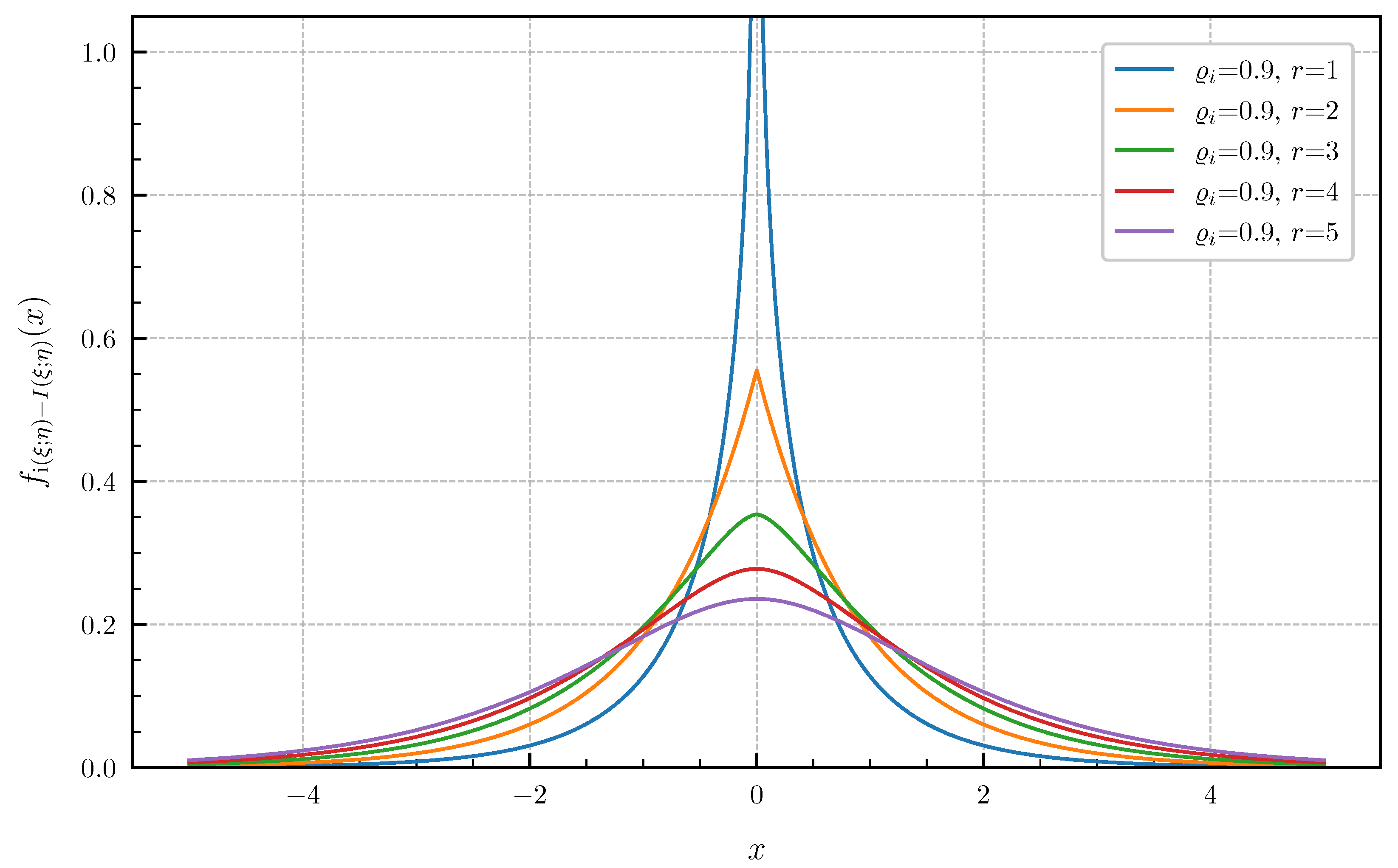
Figure 2.
CDF for equal canonical correlations .

Figure 3.
PDF for equal canonical correlations .
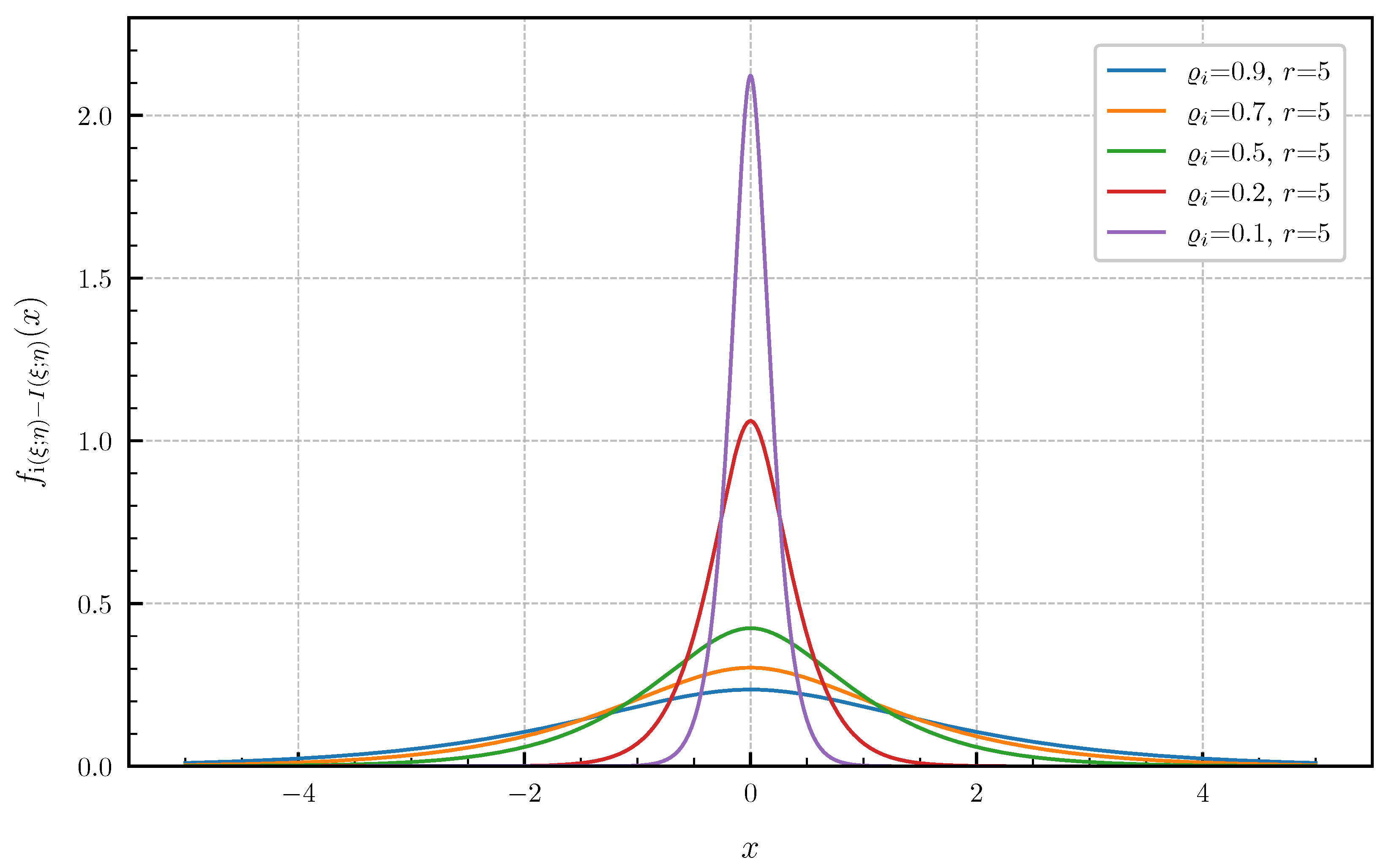
Figure 4.
CDF for equal canonical correlations .

Figure 5.
PDF for equal canonical correlations vs. Gaussian approximation.
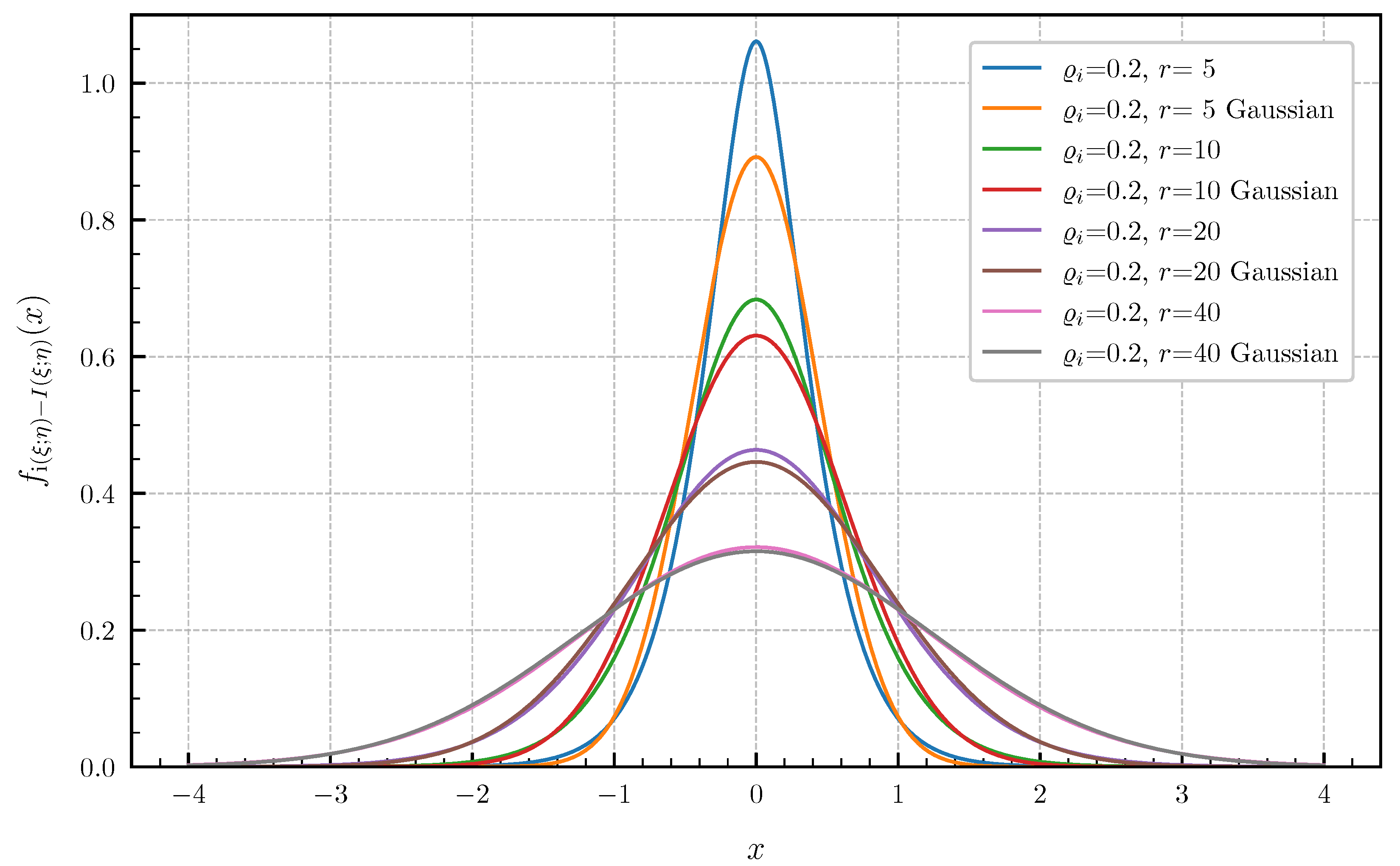
Figure 6.
CDF for equal canonical correlations vs. Gaussian approximation.

Figure 7.
Approximated PDF for canonical correlations given in (70) for and (approximation error ) vs. Gaussian approximation ().
Figure 7.
Approximated PDF for canonical correlations given in (70) for and (approximation error ) vs. Gaussian approximation ().
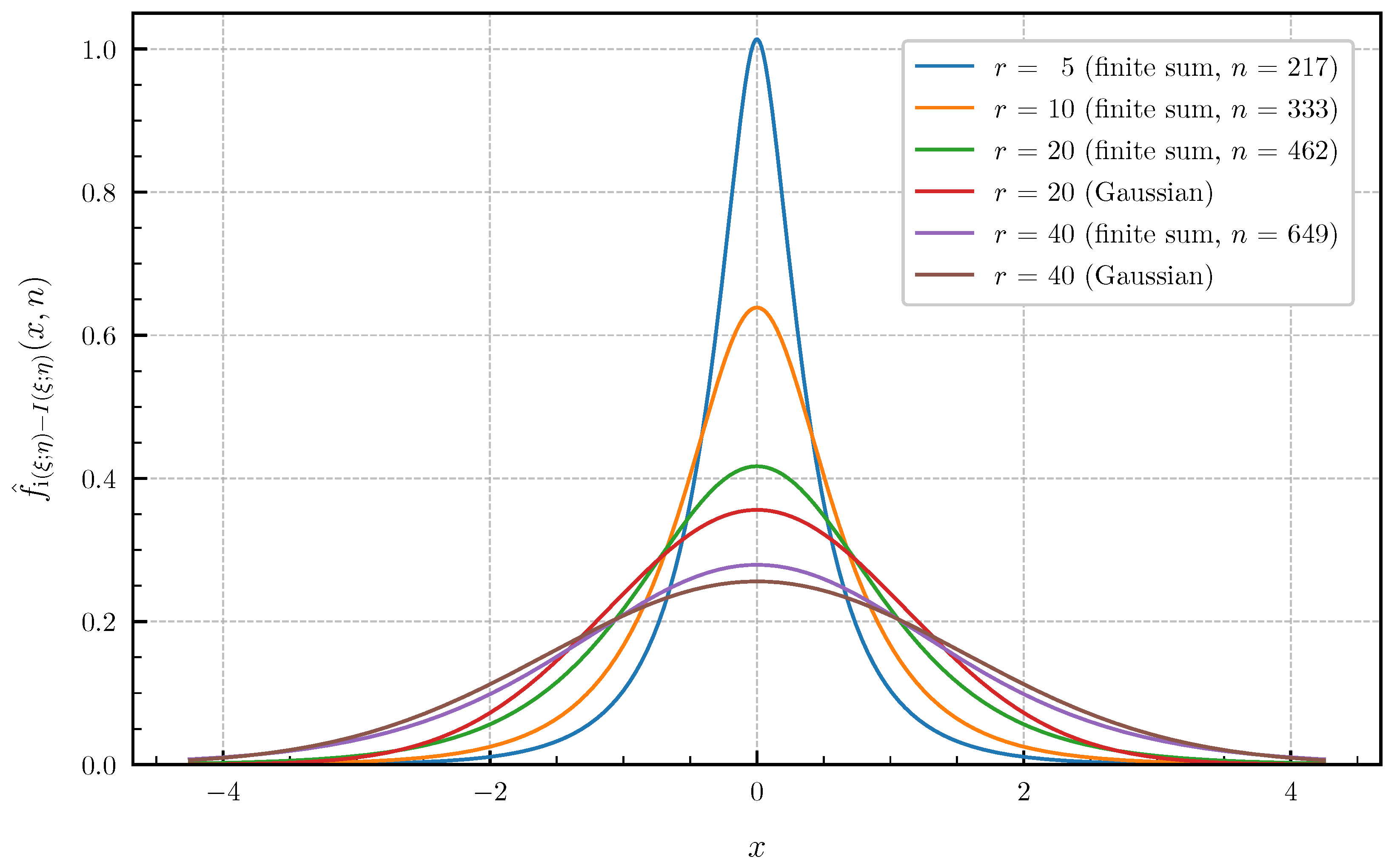
Figure 8.
Approximated CDF for canonical correlations given in (70) for and (approximation error ) vs. Gaussian approximation ().
Figure 8.
Approximated CDF for canonical correlations given in (70) for and (approximation error ) vs. Gaussian approximation ().
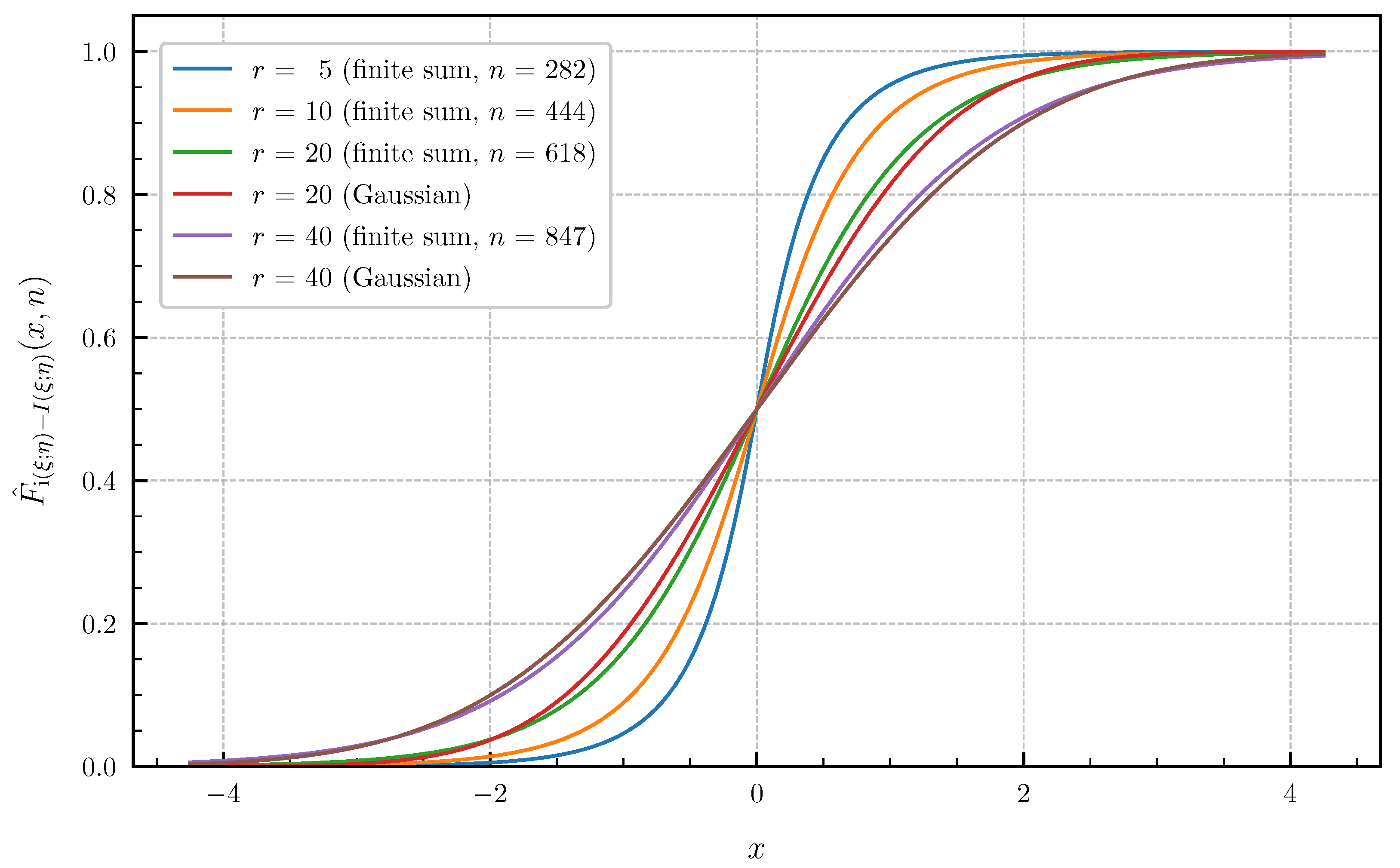
Figure 9.
Approximated PDF for canonical correlations given in (71) for (approximation error ) vs. Gaussian approximation ().
Figure 9.
Approximated PDF for canonical correlations given in (71) for (approximation error ) vs. Gaussian approximation ().

Figure 10.
Approximated CDF for canonical correlations given in (71) for (approximation error ) vs. Gaussian approximation ().
Figure 10.
Approximated CDF for canonical correlations given in (71) for (approximation error ) vs. Gaussian approximation ().

Publisher’s Note: MDPI stays neutral with regard to jurisdictional claims in published maps and institutional affiliations. |
© 2022 by the authors. Licensee MDPI, Basel, Switzerland. This article is an open access article distributed under the terms and conditions of the Creative Commons Attribution (CC BY) license (https://creativecommons.org/licenses/by/4.0/).
Share and Cite
MDPI and ACS Style
Huffmann, J.E.W.; Mittelbach, M. On the Distribution of the Information Density of Gaussian Random Vectors: Explicit Formulas and Tight Approximations. Entropy 2022, 24, 924. https://doi.org/10.3390/e24070924
AMA Style
Huffmann JEW, Mittelbach M. On the Distribution of the Information Density of Gaussian Random Vectors: Explicit Formulas and Tight Approximations. Entropy. 2022; 24(7):924. https://doi.org/10.3390/e24070924
Chicago/Turabian StyleHuffmann, Jonathan E. W., and Martin Mittelbach. 2022. "On the Distribution of the Information Density of Gaussian Random Vectors: Explicit Formulas and Tight Approximations" Entropy 24, no. 7: 924. https://doi.org/10.3390/e24070924
Note that from the first issue of 2016, this journal uses article numbers instead of page numbers. See further details here.