Spherical Fuzzy Logarithmic Aggregation Operators Based on Entropy and Their Application in Decision Support Systems


1
School of Economic and Management, Nanjing University of Aeronautics and Astronautics, Nanjing 211106, China
2
Department of Mathematics, Abdul Wali Khan University, Mardan 23200, Pakistan
*
Author to whom correspondence should be addressed.
Entropy 2019, 21(7), 628; https://doi.org/10.3390/e21070628
Submission received: 2 June 2019
/
Revised: 20 June 2019
/
Accepted: 23 June 2019
/
Published: 26 June 2019
(This article belongs to the Special Issue Information Theory Based Error and Regularization Functions in Artificial Intelligence Algorithms in the Big Data Era)
Abstract
:Keeping in view the importance of new defined and well growing spherical fuzzy sets, in this study, we proposed a novel method to handle the spherical fuzzy multi-criteria group decision-making (MCGDM) problems. Firstly, we presented some novel logarithmic operations of spherical fuzzy sets (SFSs). Then, we proposed series of novel logarithmic operators, namely spherical fuzzy weighted average operators and spherical fuzzy weighted geometric operators. We proposed the spherical fuzzy entropy to find the unknown weights information of the criteria. We study some of its desirable properties such as idempotency, boundary and monotonicity in detail. Finally, the detailed steps for the spherical fuzzy decision-making problems were developed, and a practical case was given to check the created approach and to illustrate its validity and superiority. Besides this, a systematic comparison analysis with other existent methods is conducted to reveal the advantages of our proposed method. Results indicate that the proposed method is suitable and effective for the decision process to evaluate their best alternative.
1. Introduction
The complication of a system is growing every day in real life and getting the finest option from the set of possible ones is difficult for the decision makers. To attain a single objective is difficult to summarize but not incredible. Many organizations found difficulties with setting motivations, goals and opinions’ complications. Thus, organizational decisions simultaneously include numerous objectives, whether they regard individuals or committees. This reflection suggests, according to criteria solved optionally, restricting each decision maker to attain an ideal solution-optimum under each criterion involved in practical problems. Consequently, the decision maker is more concentrated to establish more applicable and reliable techniques to find the best options.
To handle the ambiguity and uncertainty data in decision-making problems, the classical or crisp methods cannot be always effective. Thus, dealing with such uncertain situations, Zadeh [1] in 1965 presented the idea of the fuzzy set. Zadeh assigns membership grades to elements of a set in the interval [0,1] by offering the idea of fuzzy sets (FSs). Zadeh’s work in this direction is remarkable as many of the set theoretic properties of crisp cases were defined for fuzzy sets. Fuzzy set theory got the attention of researchers and found its applications in decision science [2], artificial intelligence [3], and medical diagnosis [4], and its enormous applications are discussed in [5].
After many applications of fuzzy set theory, Atanassov observed that there are many shortcomings in this theory and introduced the notion of intuitionistic fuzzy sets [6] to generalize the concept of Zadeh’s fuzzy set. In intuitionistic fuzzy sets, each element is expressed by an ordered pair, and each pair is characterized by membership and non-membership grades on the condition that the sum of their grades are less than or equal to 1. During the last few decades, the intuitionistic fuzzy sets (IFSs) are fruitful and broadly utilized by researchers to grasp the ambiguity and imprecision data. To cumulate all the executive of criteria for alternatives, aggregation operators play a vital role throughout the information merging procedure. Xu [7] presented a weighted averaging operator while Xu and Yager [8] developed a geometric aggregation operator for aggregating the different intuitionistic fuzzy numbers. Verma [9] in 2015 proposed the generalized Bonferroni mean operator and, in [10], Verma and Sharma proposed the measure of inaccuracy using intuitionistic fuzzy information. Deschrijver [11] developed the IFS representation of t-norms and t-conorms. In some decision theories, the decision makers deal with the situation of particular attributes where values of their summation of membership degrees exceeds 1. In such conditions, IFS has no ability to obtain any satisfactory result. To overcome this situation, Yager [12] developed the idea of a Pythagorean fuzzy set (PyFS) as a generalization of IFS, which satisfies the fact that the value of square summation of its membership degrees is less then or equal to 1. Clearly, PyFS is more flexible than IFS to deal with the imprecision and ambiguity in the practical multi-criteria decision-making (MCDM) problems. Zhang and Xu [13] established an extension of TOPSIS to MCDM with PyFS information. The error for the proof of distance measure in Zhang and Xu [13] has been pointed out by Yang et al. [14]. For MCDM problems in a Pythagorean fuzzy environment, Yager and Abbasov [15] developed a series of aggregation operators. Peng and Yang [16] explained their relationship among these aggregation operators and established the superiority and inferiority ranking (SIR) for the multi-criteria group decision-making (MCGDM) method. Using Einstein operation, Garg [17] generalized Pythagorean fuzzy information aggregation. Gou et al. [18] studied many Pythagorean fuzzy functions and investigated their fundamental properties such as continuity, derivatively, and differentiability in detail. Zhang [19] put forward a ranked qualitative flexible (QUALIFLEX) multi-criteria approach with the closeness index-based ranking methods for multi-criteria Pythagorean fuzzy decision analysis. Zeng et al. [20] explored a hybrid method for Pythagorean fuzzy MCDM. Zeng [21], applied the Pythagorean fuzzy probabilistic OWA (PFPOWA) operator for MAGDM problems. For more study, we refer to [22,23,24].
IFS theory and PyFS theory have been successfully applied in different areas, but there are situations that cannot be represented by it in real life, such as voting, we may face human opinions involving more answers of the type: yes, abstain, no and refusal (for example, in a democratic election station, the council issues’ 500 voting papers for a candidate. The voting results are divided into four groups accompanied with the number of papers that are vote for , abstain , vote against and refusal of voting . Here, group abstain means that the voting paper is a white paper rejecting both agree and disagree for the candidate but still takes the vote, group refusal of voting is either invalid voting papers or did not take the vote. The candidate is successful because the number of support papers is over 50% (i.e., 250).
However, at least five people said later on in their blogs that they support the candidate in the last moment because they find that the support number seems larger than the against number. Such kind of examples (in which the number of abstains is a key factor and the group refusal of voting indeed exists) happened in reality and IFS and PyFS could not handle it). Thus, Cuong [25] proposed a new notion named picture fuzzy sets, which is an extension of fuzzy sets and intuitionistic fuzzy sets. Picture fuzzy sets give three membership degrees of an element named the positive membership degree, the neutral membership degree, and the negative membership degree, respectively. The picture fuzzy set solved the voting problem successfully, and is applied to clustering [26], fuzzy inference [27], and decision-making [28,29,30,31,32,33,34,35].
The neutrosophic set is another important generalizations of the classic set, fuzzy set, intuitionistic fuzzy set and picture fuzzy set to deal with uncertainties in decision-making problems. Many authors contributed in the decision-making theory using neutrosophic information. Ashraf [36] proposed the logarithmic hybrid aggregation operators for single value neutrosophic sets. Dragan et al. [37] proposed the novel approach for the selection of power generation technology using the combinative distance-based assessment (CODAS) method. Many decision-making approaches like [38,39] make important contributions using neutrosophic information.
The picture fuzzy set becomes more famous by introducing various kinds of aggregation operators. However, it has a shortcoming in that it is only valid for the environment whose sum of degrees is less than or equal to one. However, in day-to-day life, there are many situations where this condition is ruled out. For instance, if a person giving their preference in the form of positive, neutral and negative membership degrees towards a particular object is 0.7, 0.3 and 0.5, then clearly this situation is not handling with picture fuzzy set. In order to resolve it, Ashraf [40] proposed the notion of the spherical fuzzy set. For instance, corresponding to the above-considered example, we see that and hence a spherical fuzzy set (SFS) is an extension of the existing extensions of fuzzy set theories. In the spherical fuzzy set, each element can be written in the form of triplet component, and each pair is categorized by a positive membership degree, a neutral membership degree and a negative membership degree such that the sum of their square is less than or equal to one. Ashraf [41] proposed some series of spherical aggregation operators using t-norm and t-conorm and gave its applications to show the effectiveness of proposed operators. Ashraf in [42] proposed the GRA method based on a spherical linguistic fuzzy Choquet integral environment and gave its application. For more study, we refer to [43,44,45].
The logarithmic operations being good alternatives, compared with the algebraic operations, have the potential to offer similar smooth estimations as the algebraic operations. However, there is little investigation on logarithmic operations on the IFSs and PyFSs. Motivated by these ideas, we develop a spherical fuzzy MCDM method based on the logarithmic aggregation operators, with the logarithmic operations of the spherical fuzzy sets (SFSs) handling spherical fuzzy MCDM within SFSs.
Thus, the goal of this article is to propose the decision-making method for MCDM problems in which there exist the interrelationships among the criteria. The contributions of this study are:
- We develop some novel logarithmic operations for spherical fuzzy sets, which can overcome the weaknesses of algebraic operations and capture the relationship between various SFSs.
- We extend logarithmic operators to logarithmic spherical fuzzy operators, namely logarithmic spherical fuzzy weighted averaging (L-SFWA), logarithmic spherical fuzzy ordered weighted averaging (L-SFOWA), logarithmic spherical fuzzy hybrid weighted averaging (L-SFHWA), logarithmic spherical fuzzy weighted geometric (L-SFWG), logarithmic spherical fuzzy ordered weighted geometric (L-SFOWG) and logarithmic spherical fuzzy hybrid weighted geometric (L-SFHWG) to SFSs, which can overcome the algebraic operators’ drawbacks.
- We develop the spherical fuzzy entropy for spherical fuzzy information, which can help to find the unknown weights information of the criteria.
- We develop an algorithm to deal with multi-attribute decision-making problems using spherical fuzzy information.
- To show the effectiveness and reliability of the proposed spherical fuzzy logarithmic aggregation operators, the application of the proposed operator in emerging technology enterprises is developed.
- Results indicate that the proposed technique is more effective and gives more accurate output as compared to existing studies.
In order to attain the research goal that has been stated above, the organization of this article is offered as: Section 2 concentrates on some basic notions and operations of existing extensions of fuzzy set theories and also some discussion to propose the spherical fuzzy entropy. Section 3 presents some novel logarithmic operational laws of SFSs. Section 4 defines the logarithmic aggregation operators for SFNs and discusses its properties. Section 5 presents an approach for handling the spherical fuzzy MCDM problem based on the proposed logarithmic operators. Section 5.1 uses an application case to verify the novel method and Section 5.2 presents the comparison study about algebraic and logarithmic aggregation operators. Section 6 concludes the study.
2. Preliminaries
The concepts and basic operations of existing extensions of fuzzy sets are recalled in this section, and they are the foundation of this study.
Definition 1
([27]). A mapping is said to be triangular-norm if each element satisfies that:
(1) is commutative, monotonic and associative,
(2) each
where is the unite interval.
Definition 2
([27]). A mapping is said to be triangular-conorm if each element satisfies that
(1) is commutative, monotonic and associative,
(2) each
where is the unite interval.
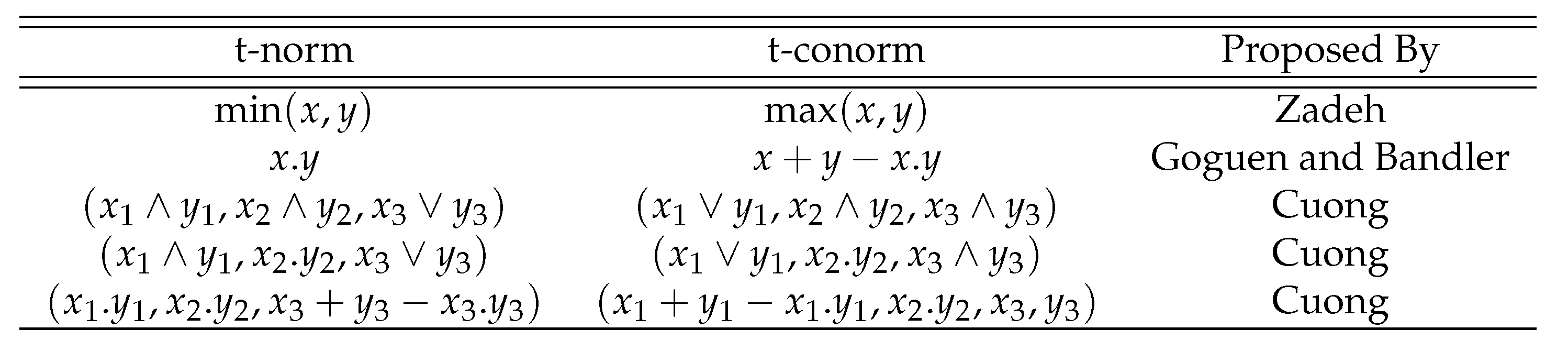
As different norms are the curial elements for proposing aggregation operators in fuzzy set theory, here we enlist some basic norms operations for fuzzy sets in Figure 1.
Definition 3
([15]). For a set ℜ, by a Pythagorean fuzzy set in ℜ, we mean a structure
in which and indicate that the positive and negative grades in are the unit intervals. In addition, the following condition satisfied by and is ; for all Then, ε is said to be a Pythagorean fuzzy set in ℜ.
Definition 4
([25]). For a set ℜ, by a picture fuzzy set in ℜ, we mean a structure
in which and indicate that the positive, neutral and negative grades in ℜ, are the unit intervals. In addition, the following condition satisfied by and is , for all Then, ε is said to be a picture fuzzy set in ℜ.
Definition 5
([40]). For a set ℜ, by a spherical fuzzy set in ℜ, we mean a structure
in which and indicate that the positive, neutral and negative grades in ℜ, are the unit intervals. In addition, the following condition satisfies by and is , for all Then, ε is said to be a spherical fuzzy set in ℜ.
is said to be a refusal degree of in ℜ, for SFS , which is triple components is said to SFN denoted by , where and , with the condition that:
Ashraf and Abdullah [40] proposed the basic operations of spherical fuzzy set as follows:
Definition 6.
For any two SFNs, and in ℜ. The union, intersection and compliment are proposed as:
(1) and ;
(2) and ;
(3)
(4)
(5)
Definition 7.
For any two SFNs, and in ℜ and then, the operations of SFNs are proposed as
(1)
(2)
(3)
(4)
(5)
Ashraf and Abdullah [40] introduced some properties based on Definition 7 as follows:
Definition 8.
For any three SFNs, , and in ℜ and Then,
(1)
(2)
(3)
(4)
(5)
(6)
(7)
(8)
Definition 9.
For any SFN, in ℜ. Then, score and accuracy values are defined as
(1)
(2)
The score and accuracy values defined above suggest which SFN is greater than other SFNs. The comparison technique is defined in the next definition.
Definition 10.
For any SFNs, in ℜ. Then, the comparison technique is proposed as
(1) If then
(2) If then
(3) If then
(a) then
(b) then
(c) then
Ashraf and Abdullah [40] proposed aggregation operators for SFNs based on different norms:
Definition 11.
For any collection of SFNs, in ℜ. The structure of the spherical weighted averaging (SFWA) operator is
where are weight vectors with and
Definition 12.
For any collection of SFNs, in ℜ. The structure of the spherical order weighted averaging (SFOWA) operator is
where are weight vectors with , and the biggest weighted value is consequently by total order
Definition 13.
For any collection of SFNs, in ℜ. The structure of the spherical hybrid weighted averaging (SFHWA) operator is
where are weight vectors with , and the biggest weighted value is consequently by total order In addition, the associated weights are with ,
Definition 14.
For any collection of SFNs, in ℜ. The structure of spherical weighted geometric (SFWG) operator is
where are weight vectors with and
Definition 15.
For any collection of SFNs, in ℜ. The structure of the spherical order weighted geometric (SFOWG) operator is
where are weight vectors with , and the biggest weighted value is consequently by total order
Definition 16.
For any collection of SFNs, in ℜ. The structure of spherical hybrid weighted geometric (SFHWG) operator is
where are weight vectors with , and the biggest weighted value is consequently by total order In addition, associated weights are with ,
3. Entropy
Basically, we familiarize the concept of entropy, when probability measures the discrimination of criteria being imposed on multi-attribute decision-making problems. Non-probabilistic entropy firstly approximated by De Luca and Termini [46] also presented some necessities to find intuitive comprehension of the degree of fuzziness. Many researchers are getting interest in this field and have done a lot of work such as Scmidt and Kacprzyk [47] proposing some axioms for distance between intuitionistic fuzzy sets and non-probabilistic entropy measure for them. In this section, we recall the concept of Shannon entropy, fuzzy entropy, entropy for Pythagorean fyzzy numbers and propose the entropy for spherical fuzzy numbers.
Definition 17
([48]). Let be the set of n-complete probability distributions. Shannon entropy for probability distribution is defined as
Definition 18
Definition 19
([49]). Let F be any fuzzy set in ℜ, and, for Pythagorean fuzzy entropy for the set F, we mean a structure
Definition 20.
Let F be any fuzzy set in ℜ, spherical fuzzy entropy for the set F, and we mean a structure
4. Spherical Fuzzy Logarithmic Operational Laws
Motivated by the novel concept of spherical fuzzy set, we introduced some novel logarithmic operational laws for SFNs. As real number system is meaningless and is not defined therefore, in our study, we take nonempty spherical fuzzy sets and where is any real number.
Definition 21.
For any SFN, in ℜ. The logarithmic spherical fuzzy number is defined as
in which and indicate that the positive, neutral and negative grades in ℜ, are the unit intervals. In addition, the following condition satisfies by and is for all Therefore, the membership grade is
the neutral grade is
and the negative grade is
Therefore,
is SPN.
Definition 22.
For any SFN, in ℜ. If
then the function is known to be a logarithmic operator for a spherical fuzzy set, and its value is called logarithmic SFN (L-SFN). Here, we take
Theorem 1.
For any SFN, in ℜ, then is also a spherical fuzzy number.
Proof.
Since any SFN in ℜ, which means that and indicate that the positive, neutral and negative grades in ℜ, are the unit intervals. In addition, the following condition satisfied by and is The following two cases happen.
Case-1 When and since is a decreasing function w.r.t Thus, and hence , and Therefore, is SFN.
Case-2 When , and similar to the above, we can find that is SFN. Thus, the procedure is eliminated here. □
Example 1.
Suppose that, for any SFN, in ℜ with then
In addition, if , then it follows:
Now, we give some discussion on the basic properties of the L-SFN.
Theorem 2.
For any SFN, in ℜ. If then
(1)
(2)
Proof.
(1) According to Definitions 7 and 22, we obtain
(2) According to Definition 22, we obtain
□
Definition 23.
For any two L-SFNs, and in ℜ and then the logarithmic operations of L-SFNs are proposed:
(1)
(2)
(3)
(4)
Theorem 3.
For any two L-SFNs, in ℜ, with Then,
(1)
(2)
Proof.
This is straightforward from Definition 23, so the procedure is eliminated here. □
Theorem 4.
For any two L-SFNs, in ℜ, with Then,
(1)
(2)
Proof.
This is straightforward from Definition 23, so the procedure is eliminated here. □
Theorem 5.
For any two L-SFNs, in ℜ, with be any real numbers. Then,
(1)
(2)
(3)
(4)
(5)
Proof.
(1) Since, from Definition 23, we have
for any real number we obtain
(2) Since, from Definition 23, we have
for any real number we obtain
(3) and (4) are similarly as above, so the procedure is eliminated here.
(5) Since, from Definition 23, we have
this is therefore proved. □
Definition 24.
For any L-SFN, in ℜ. Then, score and accuracy values are defined as
(1)
(2)
The score and accuracy values defined above suggest which L-SFN is greater than other L-SFNs. The comparison technique is defined in the next definition.
Definition 25.
For any L-SFN, in ℜ. Then, the comparison technique is proposed as
(1) If then
(2) If then
(3) If then
(a) then
(b) then
(c) then
5. Logarithmic Aggregation Operators for L-SFNs
Now, we propose novel spherical fuzzy logarithmic aggregation operators for L-SFNs based on defined spherical fuzzy logarithmic operations laws as follows:
5.1. Logarithmic Averaging Operators
Definition 26.
For any collection of SFNs, in ℜ, with The structure of logarithmic spherical weighted averaging (L-SFWA) operator is
where are weight vectors with and
Theorem 6.
For any collection of SFNs, in ℜ, with Then, by using logarithmic operations and Definition 26, is defined as
where are weight vectors with and
Proof.
Using mathematical induction to prove Theorem 6, we therefore proceed as follows:
(a) For , since
and
Then,
(b) Now, Theorem 6 is true for ,
(c) Now, we prove that Theorem 6 for which is
Thus, Theorem 6 is true for . Hence, it is satisfied for all n. Therefore,
In a similar way, if we can also obtain
which completes the proof. □
Remark 1.
If that is then the operator is reduced as follows:
Properties: The operator satisfies some properties that are listed below:
(1) Idempotency: For any collection of SFNs, in ℜ. Then, if the collection of SFNs is identical,
(2) Boundedness: For any collection of SFNs, in ℜ. and in ℜ, therefore
(3) Monotonically: For any collection of SFNs, in ℜ.If for then
Definition 27.
For any collection of SFNs, in ℜ, with The structure of the logarithmic spherical ordered weighted averaging (L-SFOWA) operator is
where are weight vectors with and and the biggest weighted value is consequently by total order
Theorem 7.
For any collection of SFNs, in ℜ, with Then, by using logarithmic operations and Definition 27, is defined as
where are weight vectors with and and the biggest weighted value is consequently by total order
Proof.
The proof is similar to Theorem 6. Thus, the procedure is eliminated here. □
Remark 2.
If that is, then the operator is reduced as follows:
Properties: The operator satisfies some properties that are listed below:
(1) Idempotency: For any collection of SFNs, in ℜ.Then, if a collection of SFNs is identical, that is,
(2) Boundedness: For any collection of SFNs, in ℜ. and in ℜ; therefore,
(3) Monotonically: For any collection of SFNs, in ℜ. If for then
Definition 28.
For any collection of SFNs, in ℜ, with The structure of a logarithmic spherical hybrid weighted averaging (L-SFHWA) operator is
where are weight vectors with and and the biggest weighted value is consequently by total order In addition, associated weights are with ,
Theorem 8.
For any collection of SFNs, in ℜ, with Then, by using logarithmic operations and Definition 28, is defined as
where are weight vectors with and and the biggest weighted value is consequently by total order In addition, associated weights are with ,
Proof.
This proof issimilar to Theorem 6, so the procedure is eliminated here. □
Remark 3.
If that is, then the operator reduces to
Properties: The operator satisfies some properties that are listed below:
(1) Idempotency: For any collection of SFNs, in ℜ. Then, if a collection of SFNs are identical, that is,
(2) Boundedness: For any collection of SFNs, in ℜ. and in ℜ; therefore,
(3) Monotonically: For any collection of SFNs, in ℜ.If for then
5.2. Logarithmic Geometric Operators
Definition 29.
For any collection of SFNs, in ℜ, with The structure of logarithmic spherical weighted geometric (L-SFWG) operator is
where are weight vectors with and
Theorem 9.
For any collection of SFNs, in ℜ, with Then, by using logarithmic operations and Definition 29, is defined as
where are weight vectors with and
Proof.
Using mathematical induction to prove Theorem 9, we proceed as follows:
(a) For , since
and
then
(b) Now, Theorem 9 is true for ,
(c) Now, we prove that Theorem 9 for that is,
Thus, Theorem 9 is true for . Hence, it is satisfied for all n. Therefore,
In a similar way, if we can also obtain
which completes the proof. □
Remark 4.
If that is, then the operator reduces to
Properties: The operator satisfies some properties that are listed below:
(1) Idempotency: For any collection of SFNs, in ℜ.Then, if a collection of SFNs are identical, that is,
(2) Boundedness: For any collection of SFNs, in ℜ. and in ℜ, therefore
(3) Monotonically: For any collection of SFNs, in ℜ.If for then
Definition 30.
For any collection of SFNs, in ℜ, with The structure of logarithmic spherical ordered weighted geometric (L-SFOWG) operator is
where are weight vectors with and and the biggest weighted value is consequently by total order
Theorem 10.
For any collection of SFNs, in ℜ, with Then, by using logarithmic operations and Definition 30, defined as
where are weight vectors with and and the biggest weighted value is consequently by total order
Proof.
This proof is similar to Theorem 9, so the procedure is eliminated here.□
Remark 5.
If that is, then operator reduces to
Properties: The operator satisfies some properties that are listed below:
(1) Idempotency: For any collection of SFNs, in ℜ.Then, if the collection of SFNs is identical, that is,
(2) Boundedness: For any collection of SFNs, in ℜ. and in ℜ, therefore
(3) Monotonically: For any collection of SFNs, in ℜ. If for then
Definition 31.
For any collection of SFNs, in ℜ, with The structure of logarithmic spherical hybrid weighted geometric (L-SFHWG) operator is
where are weight vectors with and and the biggest weighted value is consequently by total order In addition, associated weights are with ,
Theorem 11.
For any collection of SFNs, in ℜ, with Then, by using logarithmic operations and Definition 31, is defined as
where are weight vectors with and and the biggest weighted value is consequently by total order In addition, the associated weights are with ,
Proof.
This proof is similar to Theorem 9. Thus, the procedure is eliminated here. □
Remark 6.
If that is, then, operator reduces to
Properties: The operator satisfies some properties that are listed below:
(1) Idempotency: For any collection of SFNs, in ℜ. Then, if collection of SFNs are identical, that is,
(2) Boundedness: For any collection of SFNs, in ℜ. and in ℜ, therefore
(3) Monotonically: For any collection of SFNs, in ℜ. If for then
6. Proposed Technique for Solving Decision-Making Problems
In this section, we propose a new approach to decision-making based on the spherical fuzzy set. This approach will use data information provided by the decision problem only and does not need any additional information provided by decision makers, in order to avoid the effect of subjective information influencing the decision results. In the following, we will introduce a spherical fuzzy set decision-making matrix as indicated below.
- Step 1:
- Let be a distinct set of m probable alternatives and be a finite set of n criteria, where indicates the alternatives and indicates the criteria. Let be a finite set of t experts, where indicates the kth expert. The expert supplies her appraisal of an alternative on an attribute as a SFNs . The experts’ information is represented by the spherical fuzzy set decision-making matrix . Assume that is a weight vector of the attribute such that and is the weight vector of the decision makers such thatWhen we construct the spherical fuzzy decision-making matrices, for decisions. Basically, criteria have two types: one is benefit criteria and the other one is cost criteria. If the spherical fuzzy decision matrices have cost type criteria matrices, can be converted into the normalized spherical fuzzy decision matrices, , where and is the complement of If all the criteria have the same type, then there is no need for normalization.Taking the decision information from the given matrix and using the operator, the individual total spherical fuzzy preference value of the alternative is derived as follows:where is the weight vector of the attribute.
- Step 2:
- In this step, we find the collective spherical information using a spherical fuzzy weighted averaging aggregation operator.
- Step 3:
- In this step, we find the weights of each of the criteria by using the spherical fuzzy entropy:
- Step 4:
- In this step, we calculate the aggregated information using all the logarithmic aggregation operators of spherical fuzzy sets.
- Step 5:
- We find the score value and the accuracy value of the cumulative overall preference value .
- Step 6:
- By the definition, rank the alternatives and choose the best alternative that has the maximum score value.
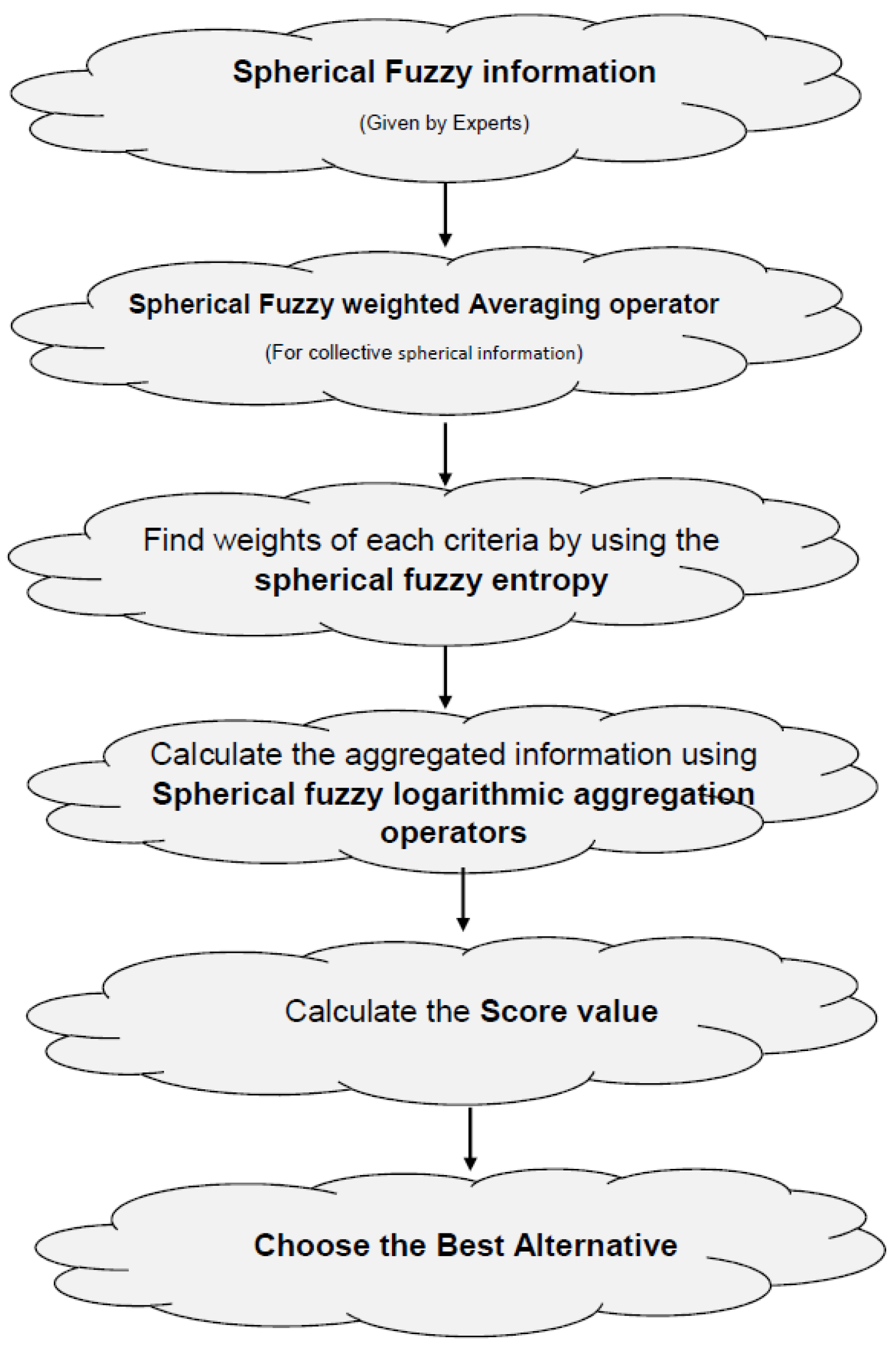
The Algorithmic Steps are shown in Figure 4.
6.1. Numerical Example
Assume that there is a committee that selects five applicable emerging technology enterprises which are given as follows:
(1) Augmented Reality ,
(2) Personalized Medicine
(3) Artificial Intelligence ,
(4) Gene Drive ,
(5) Quantum Computing
To assess the possible rising technology enterprises according to the four attributes, which are
(1) Advancement ,
(2) market risk ,
(3) financial investments and
(4) progress of science and technology .
To avoid the conflict between them, the decision makers gives the weight Construct the spherical fuzzy set decision making matrices as shown in Table 1, Table 2 and Table 3:
Since , are benefit type criteria and is cost type criteria, we need to have normalized the decision matrices. Normalized decision matrices are shown in Table 4, Table 5 and Table 6:
Step 2: Use the operator to aggregate all the individual normalized spherical fuzzy decision matrices. The aggregated spherical fuzzy decision matrix is shown in Table 7.
Step 3: The entropy of each attribute can be calculated by the following equation:
and the calculated weights are
Step 4: Now, we apply all the proposed logarithmic aggregation operators to collective spherical fuzzy information to find the aggregated information as follows:
Case-1: Using logarithmic spherical fuzzy weighted averaging aggregation operator, we obtained

Case-2: Using a logarithmic spherical fuzzy ordered weighted averaging aggregation operator, we obtained

Case-3: Using a logarithmic spherical fuzzy hybrid weighted averaging aggregation operator, we obtained

Case-4: Using a logarithmic spherical fuzzy weighted geometric aggregation operator, we obtained

Case-5: Using a logarithmic spherical fuzzy ordered weighted geometric aggregation operator, we obtained

Case-6: Using a logarithmic spherical fuzzy hybrid weighted geometric aggregation operator, we obtained

Step 5: We find the score value and the accuracy value of the cumulative overall preference value
Case-1: Score of aggregated information for the L-SFWA Operator, and we obtained

Case-2: Score of aggregated information for the L-SFOWA Operator, and we obtained

Case-3: Score of aggregated information for the L-SFHWA Operator, and we obtained

Case-4: Score of aggregated information for the L-SFWG Operator, and we obtained

Case-5: Score of aggregated information for the L-SFOWG Operator, and we obtained

Case-6: Score of aggregated inf ormation for the L-SFHWG Operator, and we obtained

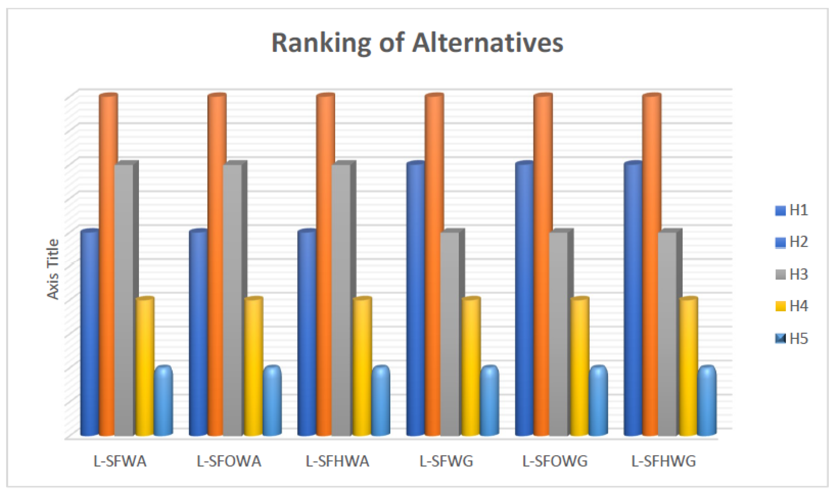
Step 6: We find the best (suitable) alternative that has the maximum score value from set of alternatives . Overall preference value and ranking of the alternatives are summarized in Table 8.
The ranking of the alternatives are shown in the Figure 5.
6.2. Sensitivity Analysis and Comparison Discussion
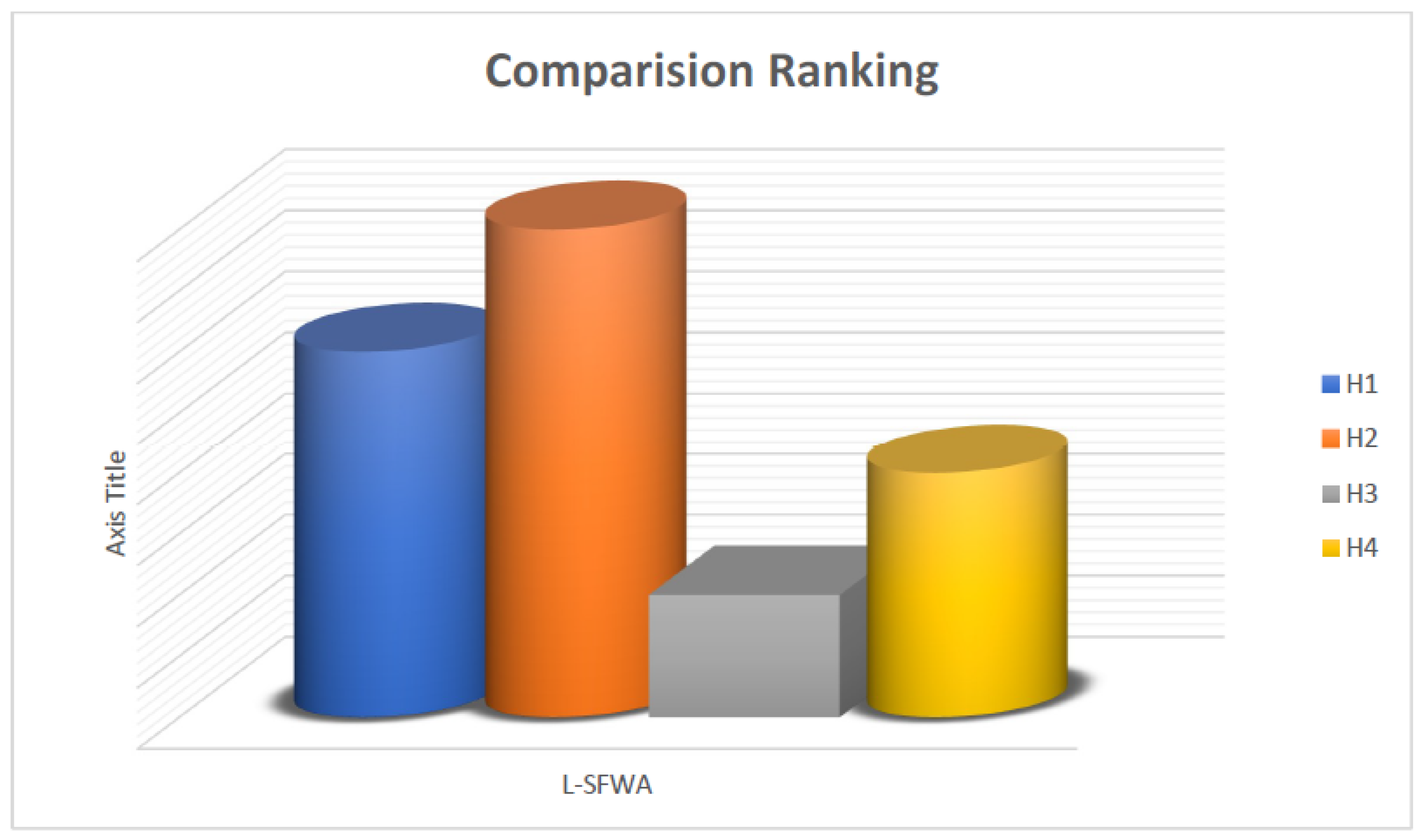
In this section, we give the comparison analysis on how our proposed logarithmic aggregation operators are effective and reliable to aggregate the spherical fuzzy information. Ashraf [40,41] proposed the spherical aggregation operators to aggregate the spherical fuzzy informatio; in this part of our study, we give a comparison between proposed and novel logarithmic spherical fuzzy aggregation operators. We take the spherical fuzzy information from [40] as follows:

Now, we utilized a logarithmic spherical fuzzy weighted averaging operator to choose the best alternative as follows:

The bast alternative is The obtained result utilizing a logarithmic spherical fuzzy weighted averaging operator is the same as results shown by Ashraf [40]. Hence, this study proposed the novel logarithmic aggregation operators to aggregate the spherical fuzzy information. This study gives a more reliable technique to aggregate and to deal with uncertainties in decision-making problems using spherical fuzzy sets. Utilizing proposed spherical fuzzy logarithmic aggregation operators, we find the best alternative from a set of alternatives given by the decision maker. Hence, the proposed MCGDM technique based on spherical fuzzy logarithmic aggregation operators gives another technique to find the best alternative as an application in decision support systems.
7. Conclusions
In this paper, we have revealed a novel logarithmic operation of SFSs with the real base number . Additionally, we have analyzed their properties and relationships. In view of these logarithmic operations, we built up the weighted averaging and geometric aggregation operators named L-SFWA, L-SFOWA, L-SFHWA, L-SFWG, L-SFOWG and L-SFHWG. A spherical fuzzy MCDM problem with interactive criteria, an approach based on the proposed operators, was proposed. Finally, this method was applied to MCDM problems. From the decision results displayed in numerical examples, we can find that our created approach can overcome the drawbacks of existing algebraic aggregation operators. In the succeeding work, we shall combine the proposed operator with some novel fuzzy sets, such as type-2 fuzzy sets, neutrosophic sets, and so on. In addition, we may investigate our created approach in the field of different areas, such as personnel evaluation, medical artificial intelligence, energy management and supplier selection evaluation. In addition, we can develop more decision-making approaches like GRA, TODAM, TOPSIS, VIKOR and so on to deal with uncertainties in the form of spherical fuzzy information.
Author Contributions
Conceptualization, S.A. (Shahzaib Ashraf) and S.A. (Saleem Abdullah); methodology, S.A. (Shahzaib Ashraf); software, S.A. (Shahzaib Ashraf); validation, S.A. (Shahzaib Ashraf), S.A. (Saleem Abdullah) and Y.J.; formal analysis, S.A. (Saleem Abdullah) and Y.J.; investigation, S.A. (Shahzaib Ashraf); writing—original draft preparation, S.A.; writing—review and editing, S.A. (Shahzaib Ashraf); visualization, Y.J.; supervision, S.A. (Saleem Abdullah); funding acquisition, Y.J.
Funding
This paper is supported by Major Humanities and Social Sciences Research Projects in Zhejiang Universities (No. 2018QN058), the China Postdoctoral Science Foundation (No. 2018QN058), the Zhejiang Province Natural Science Foundation (No. LY18G010007) and the National Natural Science Foundation of China (No. 71761027).
Acknowledgments
The authors would like to thank the editor in chief, associate editor and the anonymous referees for detailed and valuable comments that helped to improve this manuscript.
Conflicts of Interest
The authors declare no conflict of interest.
References
- Zadeh, L.A. Fuzzy sets. Inf. Control 1965, 8, 338–353. [Google Scholar] [CrossRef] [Green Version]
- Bellmann, R.E.; Zadeh, L.A. Decision making in a fuzzy environment. Manag. Sci. 1970, 17, 141–164. [Google Scholar] [CrossRef]
- Kandel, A.; Schneider, M. Fuzzy sets and their applications to artificial intelligence. Adv. Comput. 1989, 28, 69–105. [Google Scholar]
- Adlassnig, K.P. Fuzzy set theory in medical diagnosis. IEEE Trans. Syst. Man Cybern. 1986, 16, 260–265. [Google Scholar] [CrossRef]
- Dubois, D.J. Fuzzy Sets and Systems: Theory and Applications; Academic Press: New York, NY, USA, 1980. [Google Scholar]
- Atanassov, K.T. Intuitionistic fuzzy sets. Fuzzy Sets Syst. 1986, 20, 87–96. [Google Scholar] [CrossRef]
- Xu, Z. Intuitionistic fuzzy aggregation operators. IEEE Trans. Fuzzy Syst. 2007, 15, 1179–1187. [Google Scholar]
- Xu, Z.; Yager, R.R. Some geometric aggregation operators based on intuitionistic fuzzy sets. Int. J. Gen. Syst. 2006, 35, 417–433. [Google Scholar] [CrossRef]
- Verma, R. Generalized Bonferroni mean operator for fuzzy number intuitionistic fuzzy sets and its application to multiattribute decision-making. Int. J. Intell. Syst. 2015, 30, 499–519. [Google Scholar] [CrossRef]
- Verma, R.; Sharma, B.D. A new measure of inaccuracy with its application to multi-criteria decision-making under intuitionistic fuzzy environment. J. Intell. Fuzzy Syst. 2014, 27, 1811–1824. [Google Scholar]
- Deschrijver, G.; Cornelis, C.; Kerre, E.E. On the representation of intuitionistic fuzzy t-norms and t-conorms. IEEE Trans. Fuzzy Syst. 2004, 12, 45–61. [Google Scholar] [CrossRef]
- Yager, R.R. Pythagorean fuzzy subsets. In Proceedings of the Joint IFSA World Congress and NAFIPS Annual Meeting, Edmonton, AB, Canada, 24–28 June 2013; pp. 57–61. [Google Scholar]
- Zhang, X.; Xu, Z. Extension of TOPSIS to multiple criteria decision-making with Pythagorean fuzzy sets. Int. J. Intell. Syst. 2014, 29, 1061–1078. [Google Scholar] [CrossRef]
- Yang, Y.; Ding, H.; Chen, Z.S.; Li, Y.L. A note on extension of TOPSIS to multiple criteria decision-making with Pythagorean fuzzy sets. Int. J. Intell. Syst. 2016, 31, 68–72. [Google Scholar] [CrossRef]
- Yager, R.R.; Abbasov, A.M. Pythagorean membership grades, complex numbers, and decision-making. Int. J. Intell. Syst. 2013, 28, 436–452. [Google Scholar] [CrossRef]
- Peng, X.; Yang, Y. Some results for Pythagorean fuzzy sets. Int. J. Intell. Syst. 2015, 30, 1133–1160. [Google Scholar] [CrossRef]
- Garg, H. A new generalized Pythagorean fuzzy information aggregation using Einstein operations and its application to decision making. Int. J. Intell. Syst. 2016, 31, 886–920. [Google Scholar] [CrossRef]
- Gou, X.; Xu, Z.; Ren, P. The properties of continuous Pythagorean fuzzy information. Int. J. Intell. Syst. 2016, 31, 401–424. [Google Scholar] [CrossRef]
- Zhang, X. Multicriteria Pythagorean fuzzy decision analysis: A hierarchical QUALIFLEX approach with the closeness index-based ranking methods. Inf. Sci. 2016, 330, 104–124. [Google Scholar] [CrossRef]
- Zeng, S.; Chen, J.; Li, X. A hybrid method for Pythagorean fuzzy multiple-criteria decision-making. Int. J. Inf. Technol. Decis. Mak. 2016, 15, 403–422. [Google Scholar] [CrossRef]
- Zeng, S. Pythagorean fuzzy multi-attribute group decision-making with probabilistic information and OWA approach. Int. J. Intell. Syst. 2017, 32, 1136–1150. [Google Scholar] [CrossRef]
- Yager, R.R. Weighted triangular norms using generating functions. Int. J. Intell. Syst. 2004, 19, 217–231. [Google Scholar] [CrossRef]
- Rahman, K.; Abdullah, S.; Ahmed, R.; Ullah, M. Pythagorean fuzzy Einstein weighted geometric aggregation operator and their application to multiple attribute group decision-making. J. Intell. Fuzzy Syst. 2017, 33, 635–647. [Google Scholar] [CrossRef]
- Garg, H. New logarithmic operational laws and their aggregation operators for Pythagorean fuzzy set and their applications. Int. J. Intell. Syst. 2019, 34, 82–106. [Google Scholar] [CrossRef]
- Cuong, B.C. Picture Fuzzy Sets—First Results. Part 1, Seminar Neuro-Fuzzy Systems with Applications; Technical Report; Institute of Mathematics: Hanoi, Vietnam, 2013. [Google Scholar]
- Son, L.H. Generalized picture distance measure and applications to picture fuzzy clustering. Appl. Soft Comput. 2016, 46, 284–295. [Google Scholar] [CrossRef]
- Ashraf, S.; Mahmood, T.; Abdullah, S.; Khan, Q. Different approaches to multi-criteria group decision-making problems for picture fuzzy environment. Bull. Brazil. Math. Soc. New Ser. 2019, 50, 373–397. [Google Scholar] [CrossRef]
- Garg, H. Some picture fuzzy aggregation operators and their applications to multicriteria decision-making. Arab. J. Sci. Eng. 2017, 42, 5275–5290. [Google Scholar] [CrossRef]
- Phong, P.H.; Cuong, B.C. Multi-criteria Group Decision Making with Picture Linguistic Numbers. Vnu J. Sci. Comput. Sci. Commun. Eng. 2017, 32, 39–53. [Google Scholar]
- Wang, C.; Zhou, X.; Tu, H.; Tao, S. Some geometric aggregation operators based on picture fuzzy sets and their application in multiple attribute decision-making. Ital. J. Pure Appl. Math 2017, 37, 477–492. [Google Scholar]
- Wei, G. Picture fuzzy hamacher aggregation operators and their application to multiple attribute decision-making. Fund. Inform. 2018, 37, 271–320. [Google Scholar] [CrossRef]
- Cuong, B.C. Picture Fuzzy Sets—First Results. Part 2, Seminar Neuro-Fuzzy Systems with Applications; Technical Report; Institute of Mathematics: Hanoi, Vietnam, 2013. [Google Scholar]
- Si, A.; Das, S.; Kar, S. An approach to rank picture fuzzy numbers for decision-making problems. Decis. Mak. Appl. Manag. Eng. 2019. [Google Scholar] [CrossRef]
- Ashraf, S.; Abdullah, S.; Mahmood, T. Spherical fuzzy Dombi aggregation operators and their application in group decision-making problems. J. Ambient Intell. Hum. Comput. 2019, 1–19. [Google Scholar] [CrossRef]
- Ashraf, S.; Mehmood, T.; Abdullah, S.; Khan, Q. Picture Fuzzy Linguistic Sets and Their Applications for Multi-Attribute Group. Nucleus 2018, 55, 66–73. [Google Scholar]
- Ashraf, S.; Abdullah, S.; Smarandache, F. Logarithmic Hybrid Aggregation Operators Based on Single Valued Neutrosophic Sets and Their Applications in Decision Support Systems. Symmetry 2019, 11, 364. [Google Scholar] [CrossRef]
- Pamucar, D.; Badi, I.; Korica, S.; Obradovic, R. A novel approach for the selection of power generation technology using an linguistic neutrosophic combinative distance-based assessment (CODAS) method: A case study in Libya. Energies 2018, 11, 2489. [Google Scholar]
- Liu, F.; Aiwu, G.; Lukovac, V.; Vukic, M. A multicriteria model for the selection of the transport service provider: A single valued neutrosophic DEMATEL multicriteria model. Decis. Mak. Appl. Manag. Eng. 2018, 1, 121–130. [Google Scholar] [CrossRef]
- Pamučar, D.; Sremac, S.; Stević, Ž.; Ćirović, G.; Tomić, D. New multi-criteria LNN WASPAS model for evaluating the work of advisors in the transport of hazardous goods. Neural Comput. Appl. 2019, 1–24. [Google Scholar] [CrossRef]
- Ashraf, S.; Abdullah, S. Spherical aggregation operators and their application in multiattribute group decision-making. Int. J. Intell. Syst. 2019, 34, 493–523. [Google Scholar] [CrossRef]
- Ashraf, S.; Abdullah, S.; Mahmood, T.; Ghani, F.; Mahmood, T. Spherical fuzzy sets and their applications in multi-attribute decision-making problems. J. Intell. Fuzzy Syst. 2019, 36, 2829–2844. [Google Scholar] [CrossRef]
- Ashraf, S.; Abdullah, S.; Mahmood, T. GRA method based on spherical linguistic fuzzy Choquet integral environment and its application in multiattribute decisionmaking problems. Math. Sci. 2018, 12, 263–275. [Google Scholar] [CrossRef]
- Zeng, S.; Hussain, A.; Mahmood, T.; Irfan Ali, M.; Ashraf, S.; Munir, M. Covering-Based Spherical Fuzzy Rough Set Model Hybrid with TOPSIS for Multi-Attribute Decision-Making. Symmetry 2019, 11, 547. [Google Scholar] [CrossRef]
- Rafiq, M.; Ashraf, S.; Abdullah, S.; Mahmood, T.; Muhammad, S. The cosine similarity measures of spherical fuzzy sets and their applications in decision-making. J. Intell. Fuzzy Syst. 2019, 1–15, Preprint. [Google Scholar] [CrossRef]
- Khan, A.A.; Ashraf, S.; Abdullah, S.; Qiyas, M.; Luo, J.; Khan, S.U. Pythagorean Fuzzy Dombi Aggregation Operators and Their Application in Decision Support System. Symmetry 2019, 11, 383. [Google Scholar] [CrossRef]
- De Luca, A.; Termini, S. A definition of a nonprobabilistic entropy in the setting of fuzzy sets theory. Inf. Control 1972, 20, 301–312. [Google Scholar] [CrossRef] [Green Version]
- Szmidt, E.; Kacprzyk, J. Entropy for intuitionistic fuzzy sets. Fuzzy Sets Syst. 2001, 118, 467–477. [Google Scholar] [CrossRef]
- Shannon, C.E. A mathematical theory of communication. Bell Syst. Tech. J. 1948, 27, 379–423. [Google Scholar] [CrossRef]
- Chen, T.Y.; Li, C.H. Determining objective weights with intuitionistic fuzzy entropy measures: A comparative analysis. Inf. Sci. 2010, 180, 4207–4222. [Google Scholar] [CrossRef]
Figure 1.
Basic Norms Operations.

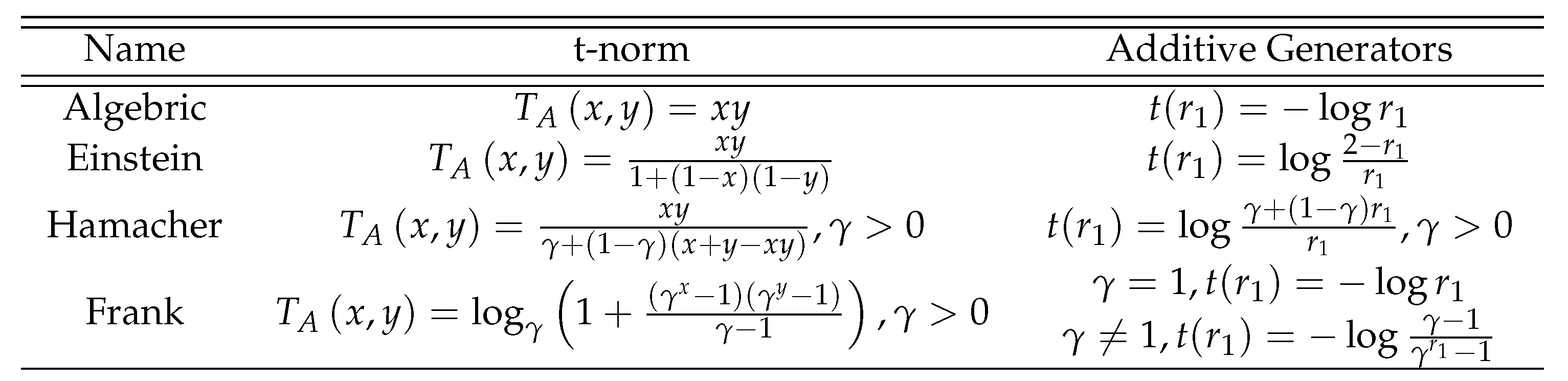
Figure 2.
T-norm with its Generators.

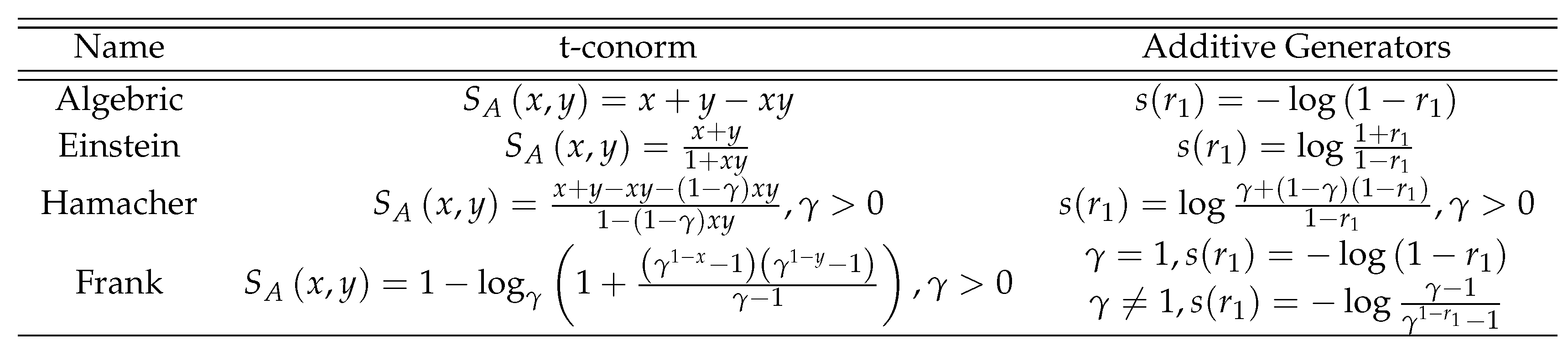
Figure 3.
T-conorm with its Generators.

Figure 4.
Algorithmic Steps.

Figure 5.
Ranking of Alternatives.

Figure 6.
Comparison Ranking.


Table 1.
Emerging technology Eenterprises .
Table 2.
Emerging technology enterprises .
Table 3.
Emerging technology enterprises .
Table 4.
Emerging technology enterprises .
Table 5.
Emerging technology enterprises .
Table 6.
Emerging technology enterprises .
Table 7.
Collective spherical fuzzy decision information matrix .
Table 8.
Overall preference value and ranking of the alternatives for .
| Ranking | ||||||
|---|---|---|---|---|---|---|
| L-SFWA | 0.985356 | 0.996515 | 0.993345 | 0.737170 | 0.920198 | |
| L-SFOWA | 0.985236 | 0.996558 | 0.993479 | 0.737233 | 0.921374 | |
| L-SFHWA | 0.999817 | 0.999998 | 0.999863 | 0.913067 | 0.996664 | |
| L-SFWG | 0.982645 | 0.988581 | 0.984383 | 0.545559 | 0.910307 | |
| L-SFOWG | 0.982461 | 0.988519 | 0.984477 | 0.544563 | 0.911435 | |
| L-SFHWG | 0.999914 | 0.999997 | 0.999657 | 0.91689 | 0.999278 |
© 2019 by the authors. Licensee MDPI, Basel, Switzerland. This article is an open access article distributed under the terms and conditions of the Creative Commons Attribution (CC BY) license (http://creativecommons.org/licenses/by/4.0/).
Share and Cite
MDPI and ACS Style
Jin, Y.; Ashraf, S.; Abdullah, S. Spherical Fuzzy Logarithmic Aggregation Operators Based on Entropy and Their Application in Decision Support Systems. Entropy 2019, 21, 628. https://doi.org/10.3390/e21070628
AMA Style
Jin Y, Ashraf S, Abdullah S. Spherical Fuzzy Logarithmic Aggregation Operators Based on Entropy and Their Application in Decision Support Systems. Entropy. 2019; 21(7):628. https://doi.org/10.3390/e21070628
Chicago/Turabian StyleJin, Yun, Shahzaib Ashraf, and Saleem Abdullah. 2019. "Spherical Fuzzy Logarithmic Aggregation Operators Based on Entropy and Their Application in Decision Support Systems" Entropy 21, no. 7: 628. https://doi.org/10.3390/e21070628
Note that from the first issue of 2016, this journal uses article numbers instead of page numbers. See further details here.