Entropy Generation of Carbon Nanotubes Flow in a Rotating Channel with Hall and Ion-Slip Effect Using Effective Thermal Conductivity Model


Abstract
:1. Introduction
2. Basic Thermal Conductivities Models for CNTs
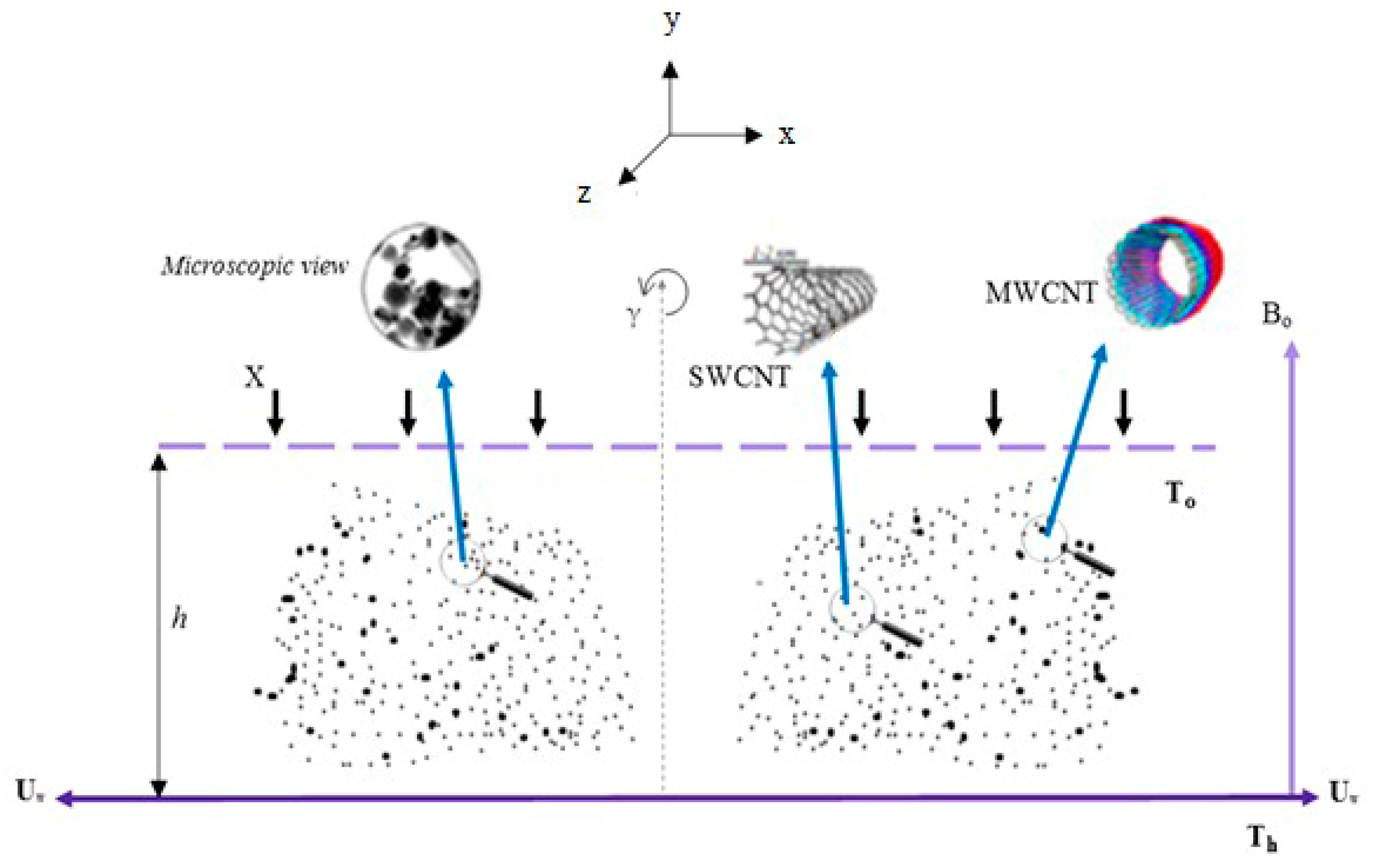
3. Mathematical Modeling
3.1. Physical Quantities of Interest
3.2. Entropy Analysis and Bejan Numbers
4. Solution by HAM
5. Results and Discussion
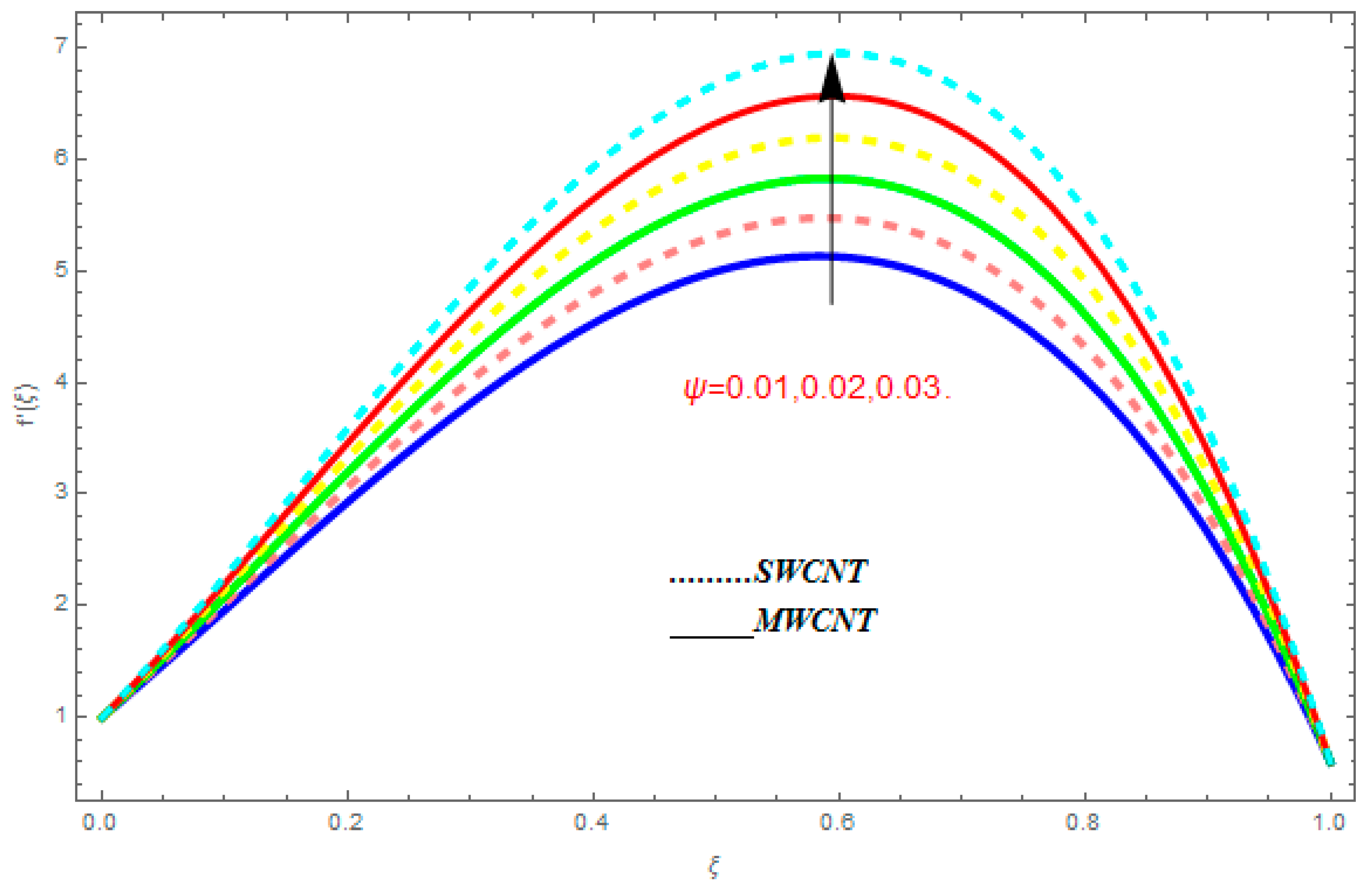
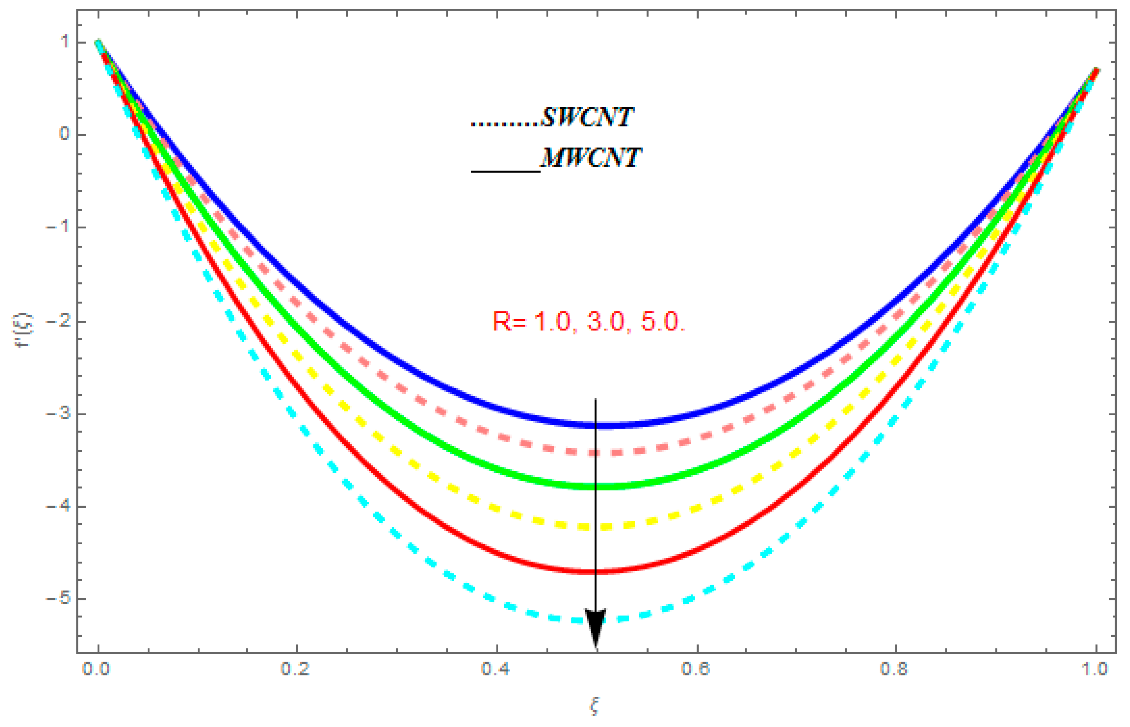
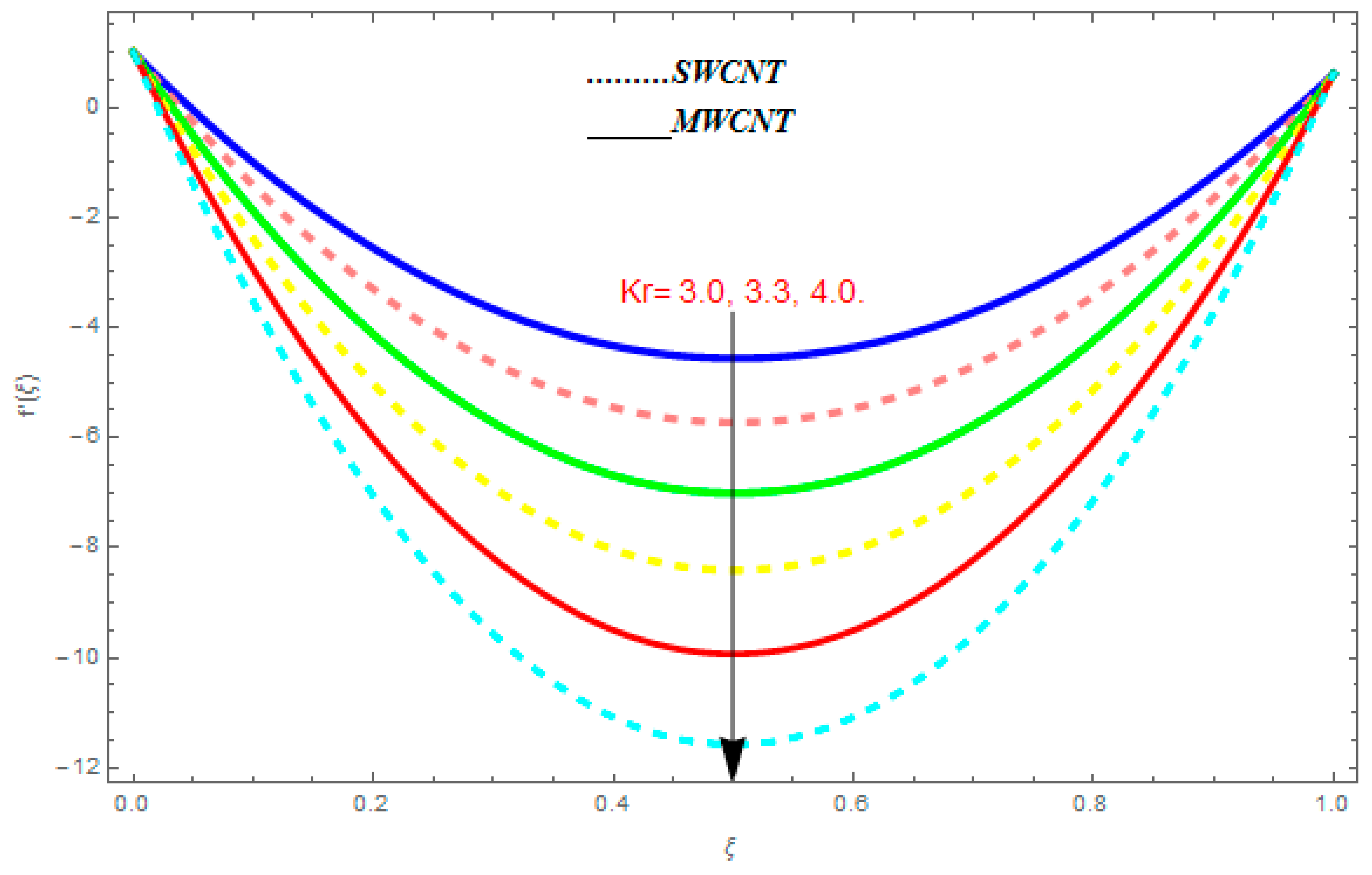
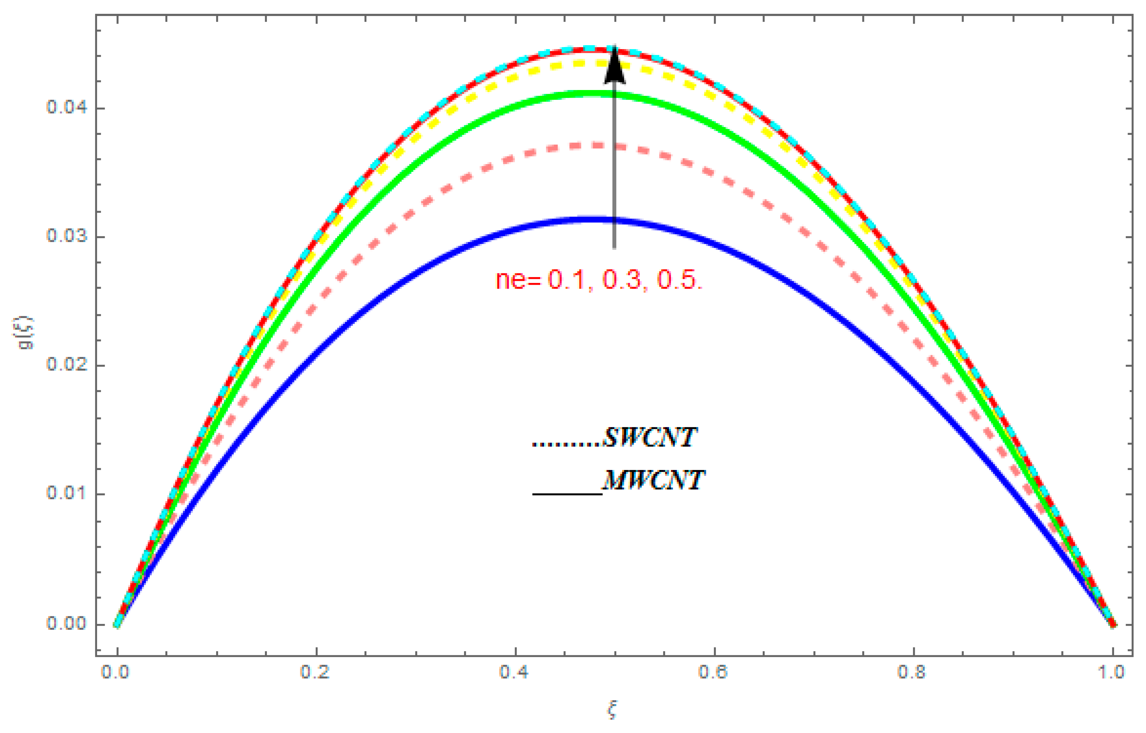
5.1. Velocity Profile
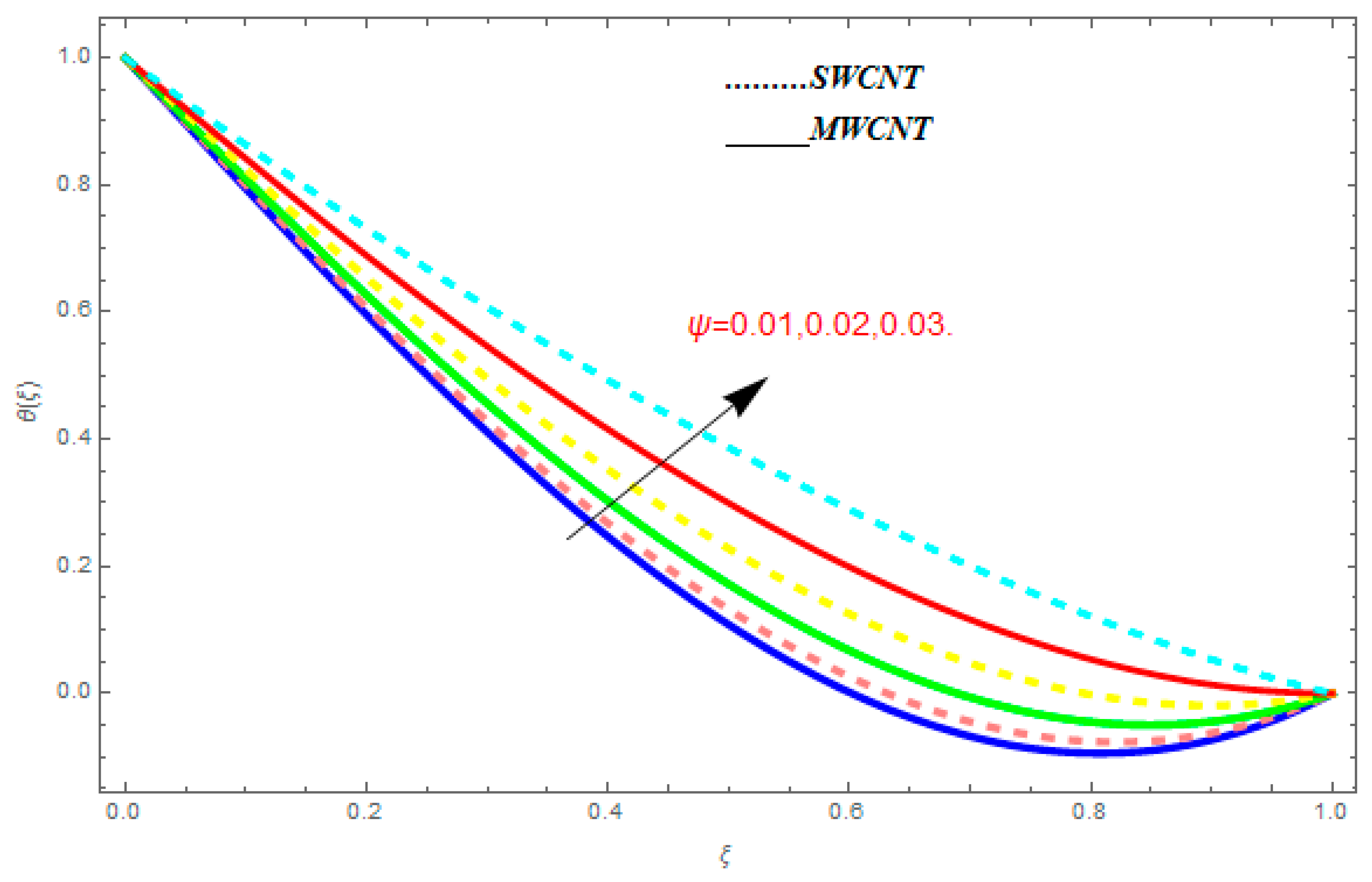
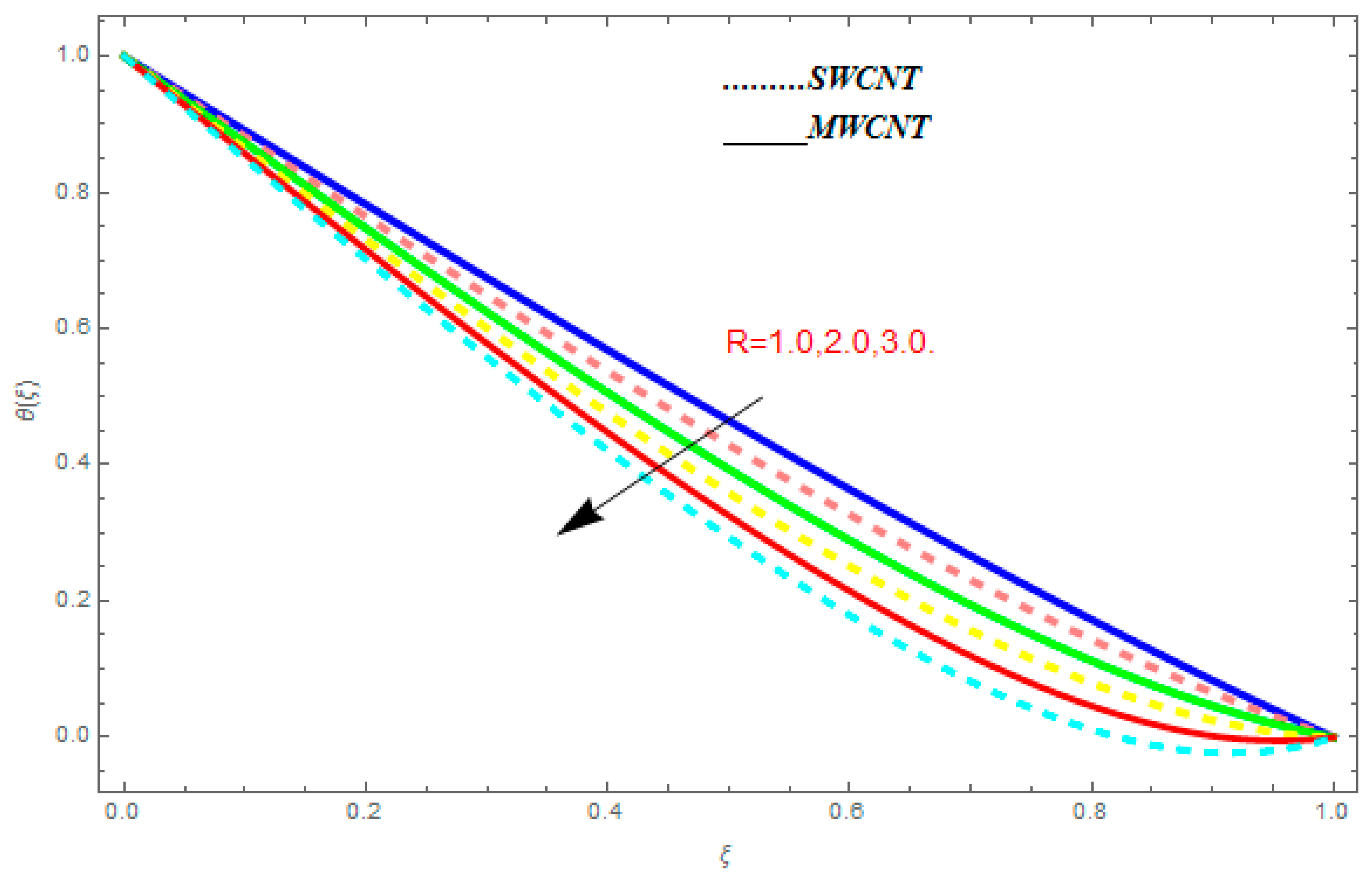
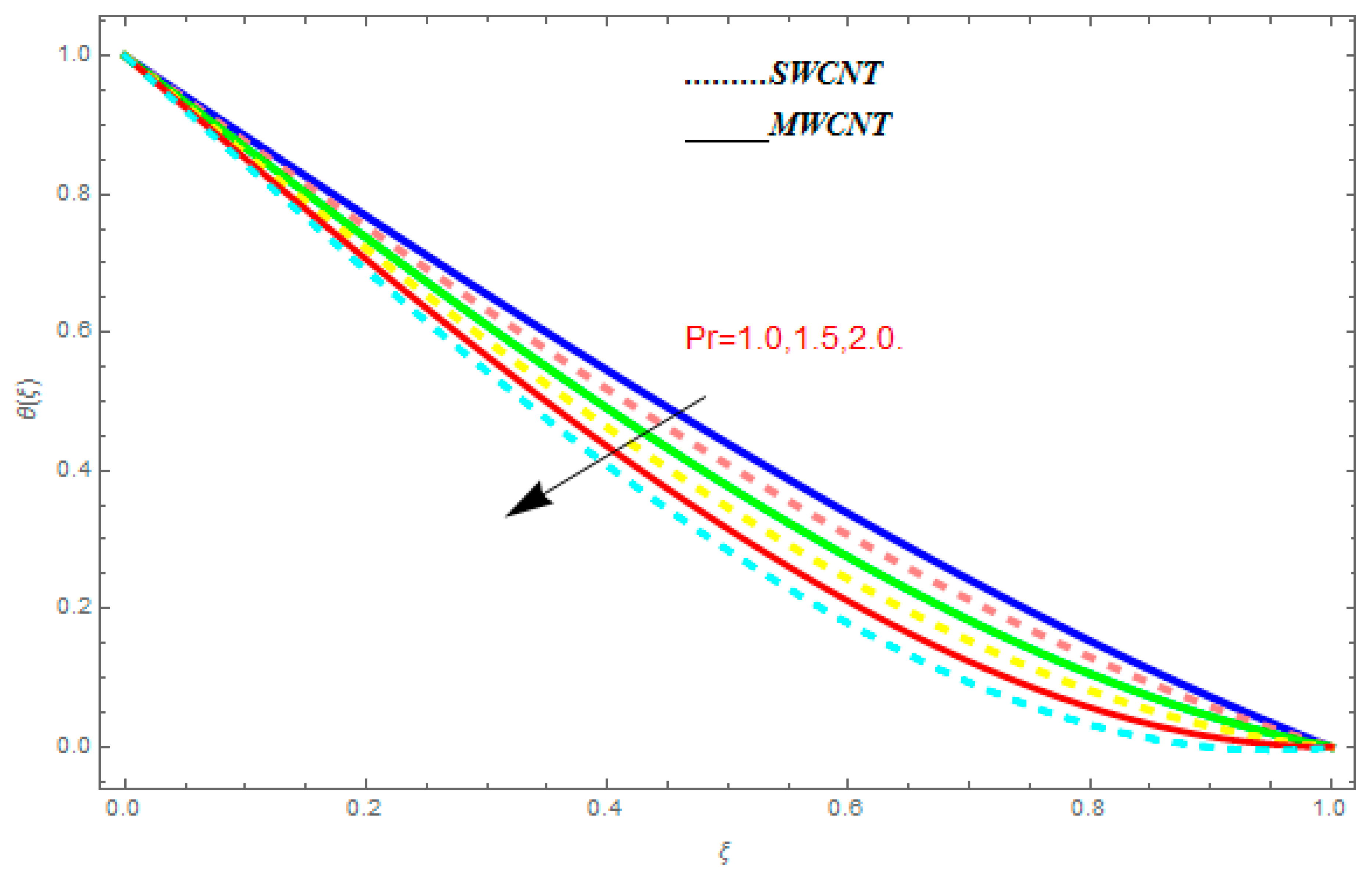
5.2. Temperature Function
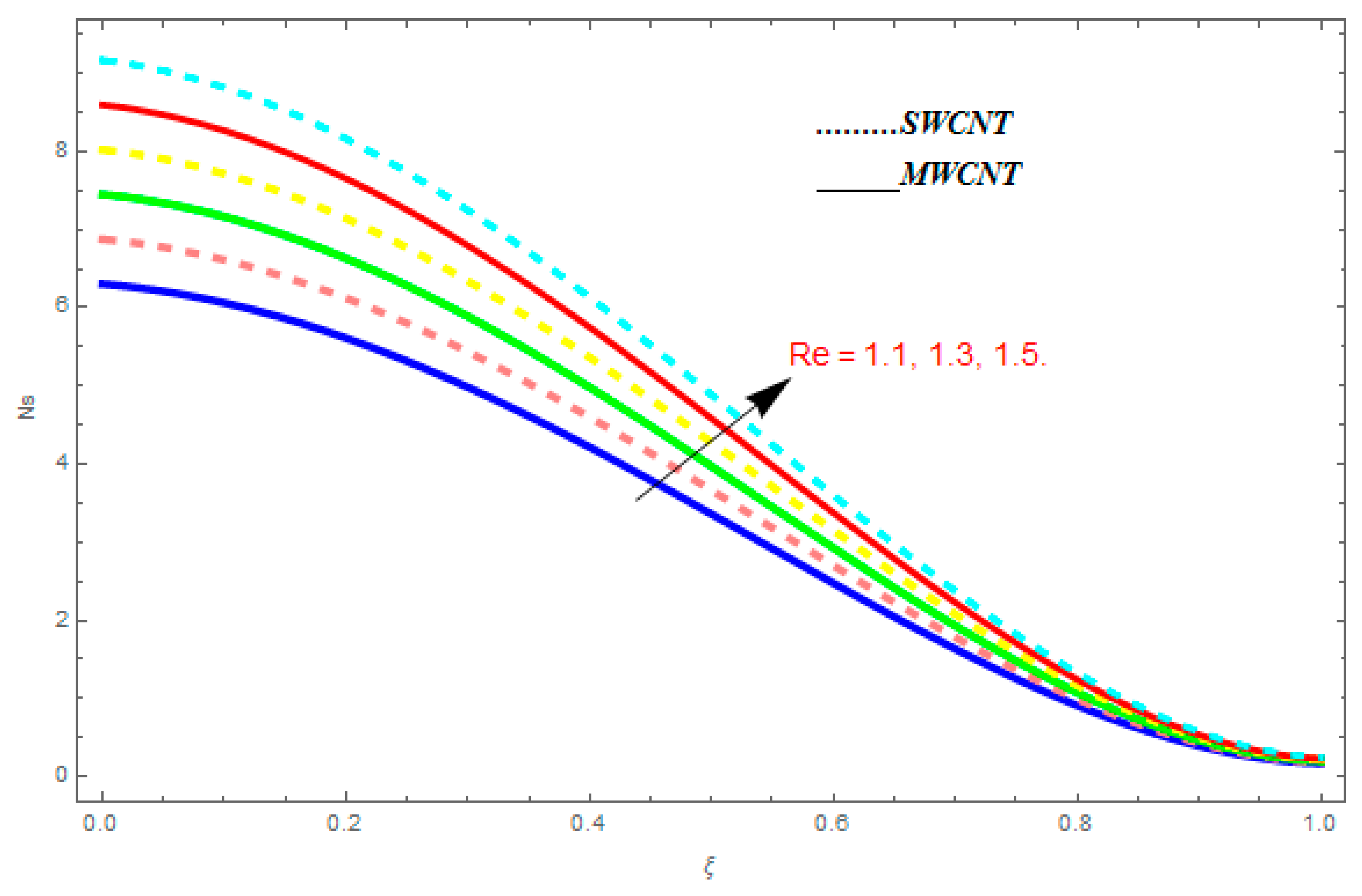
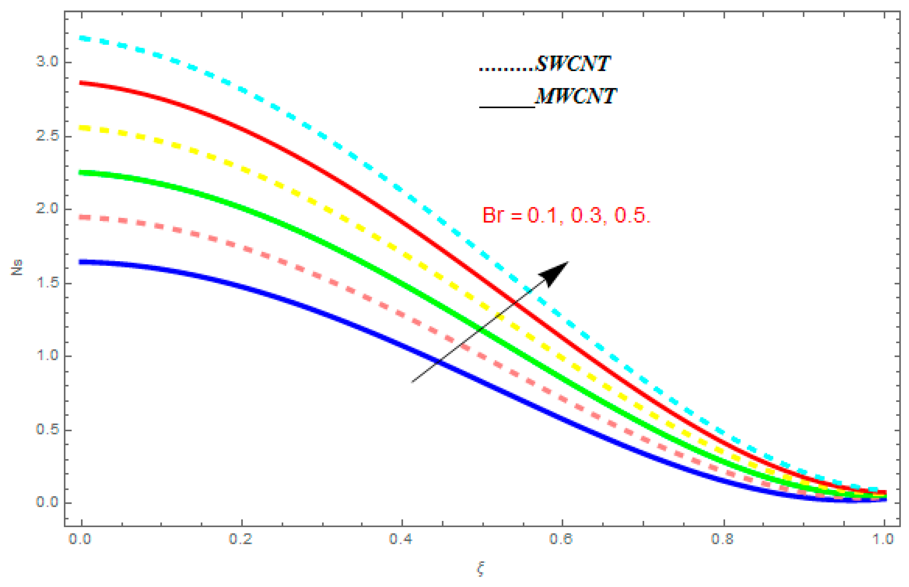
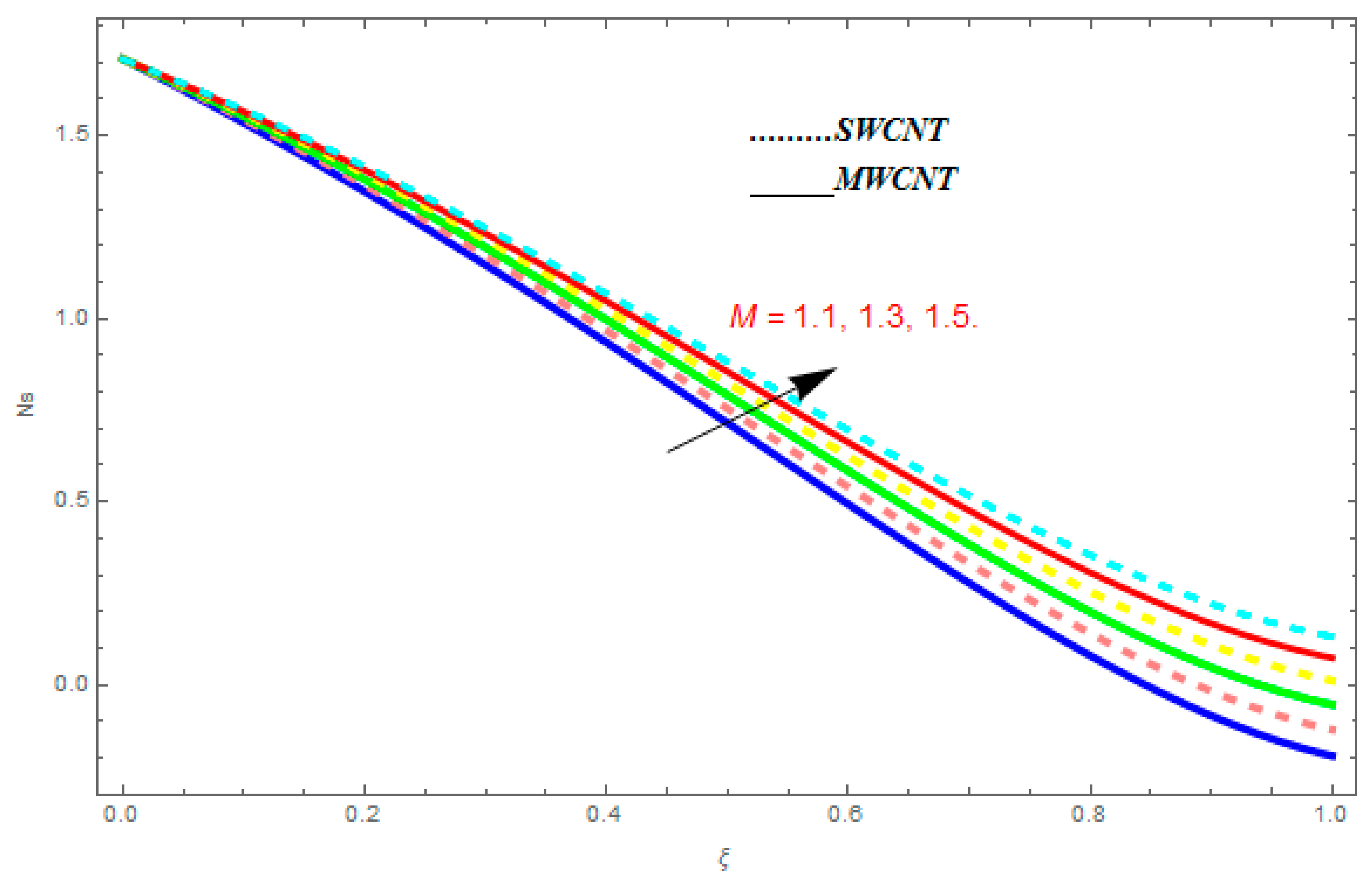
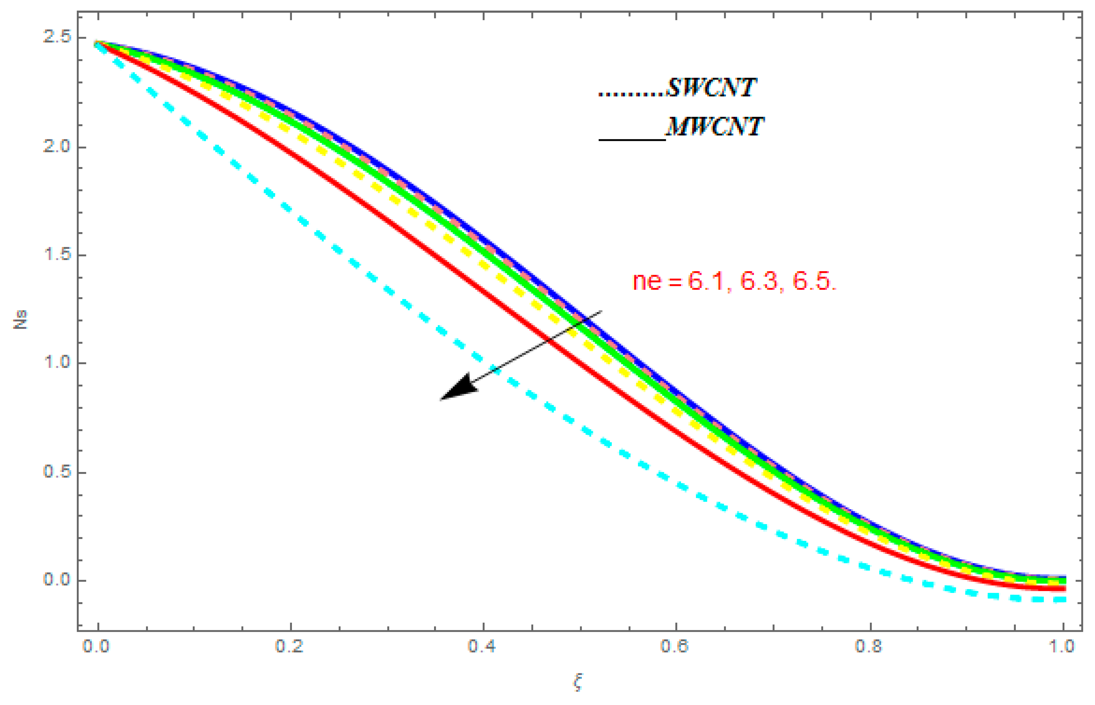
5.3. Entropy Generation () and Bejan Number ()
5.4. Tables Discussion
6. Conclusions
- (a)
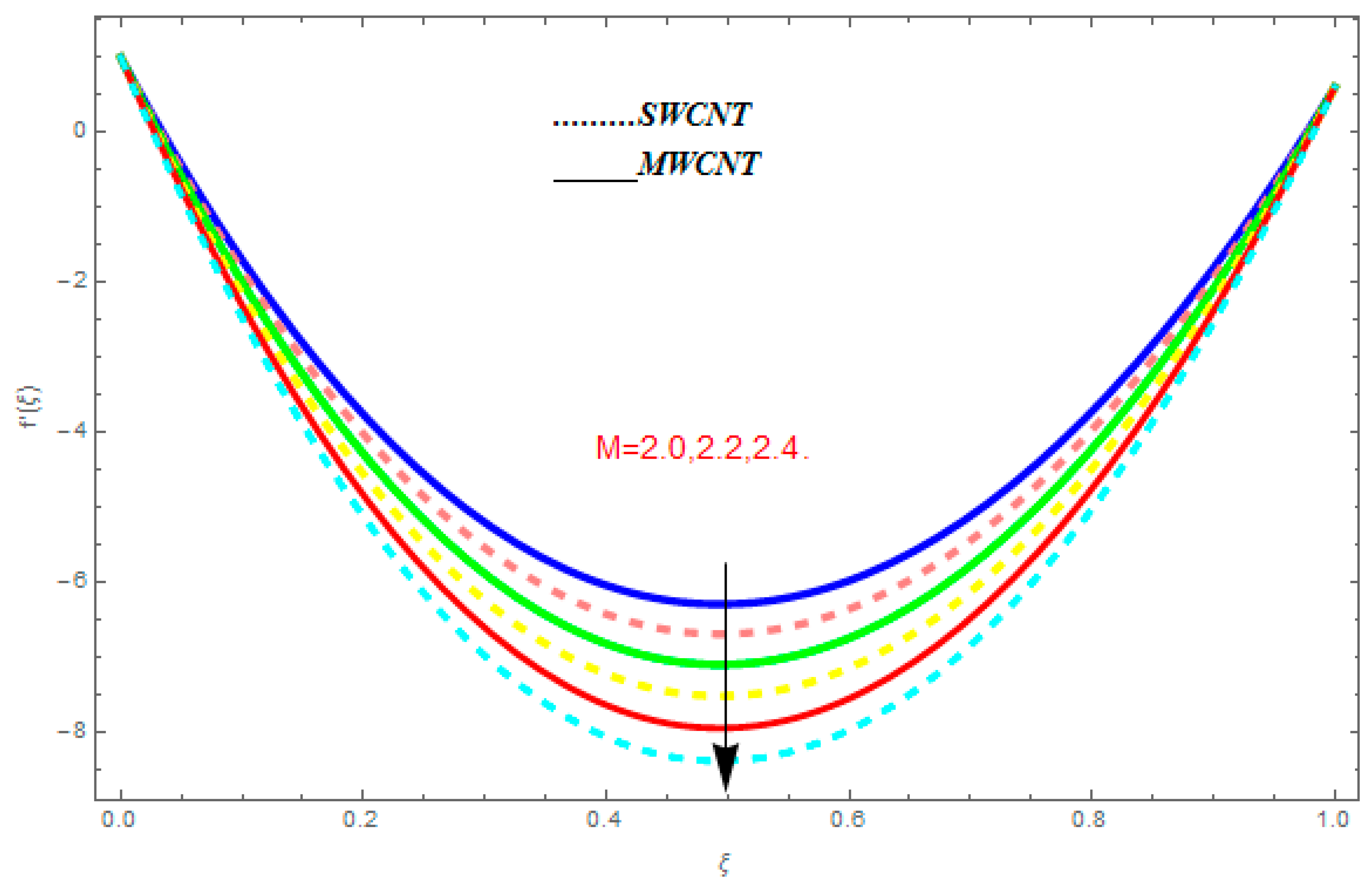
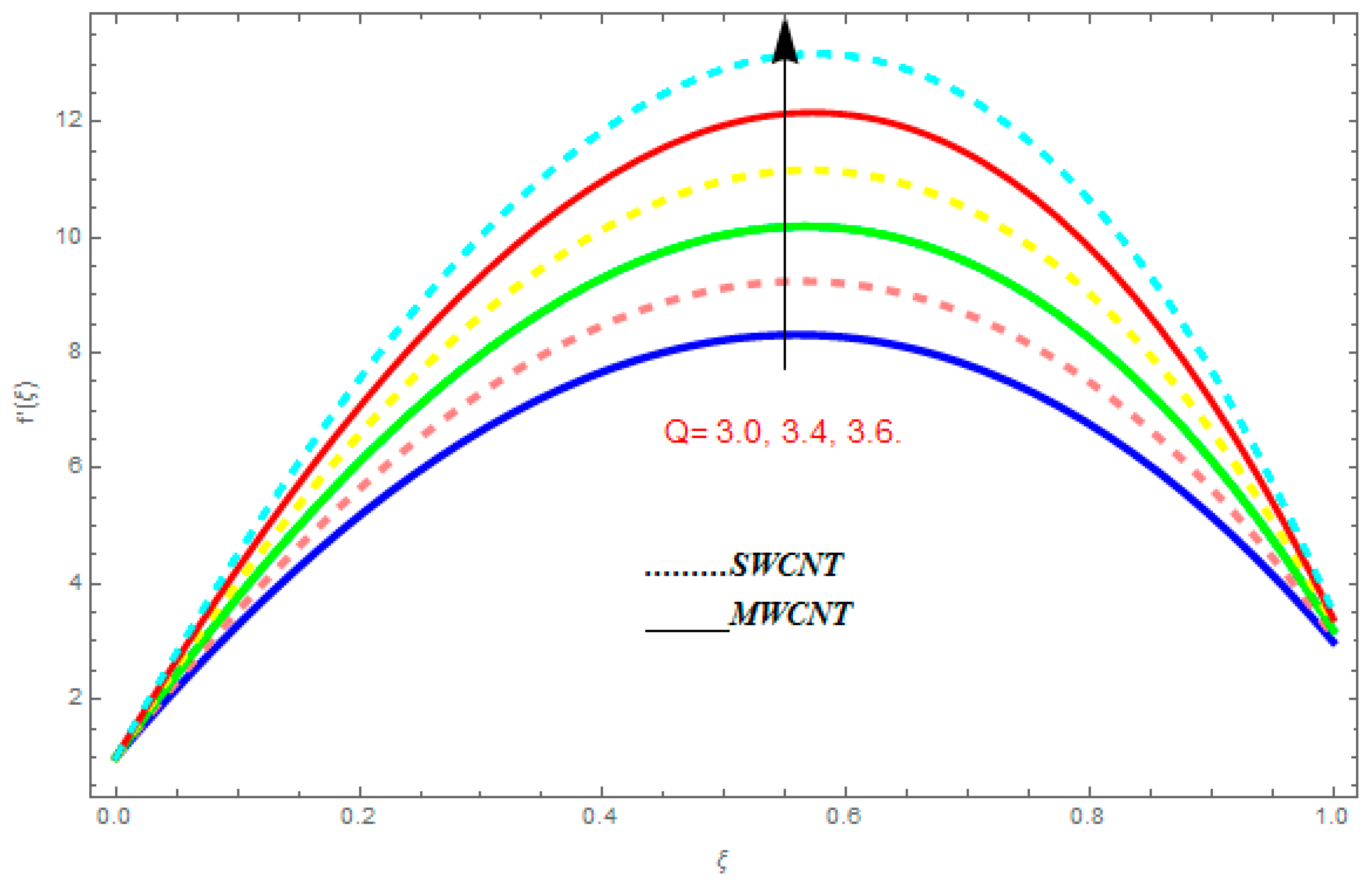
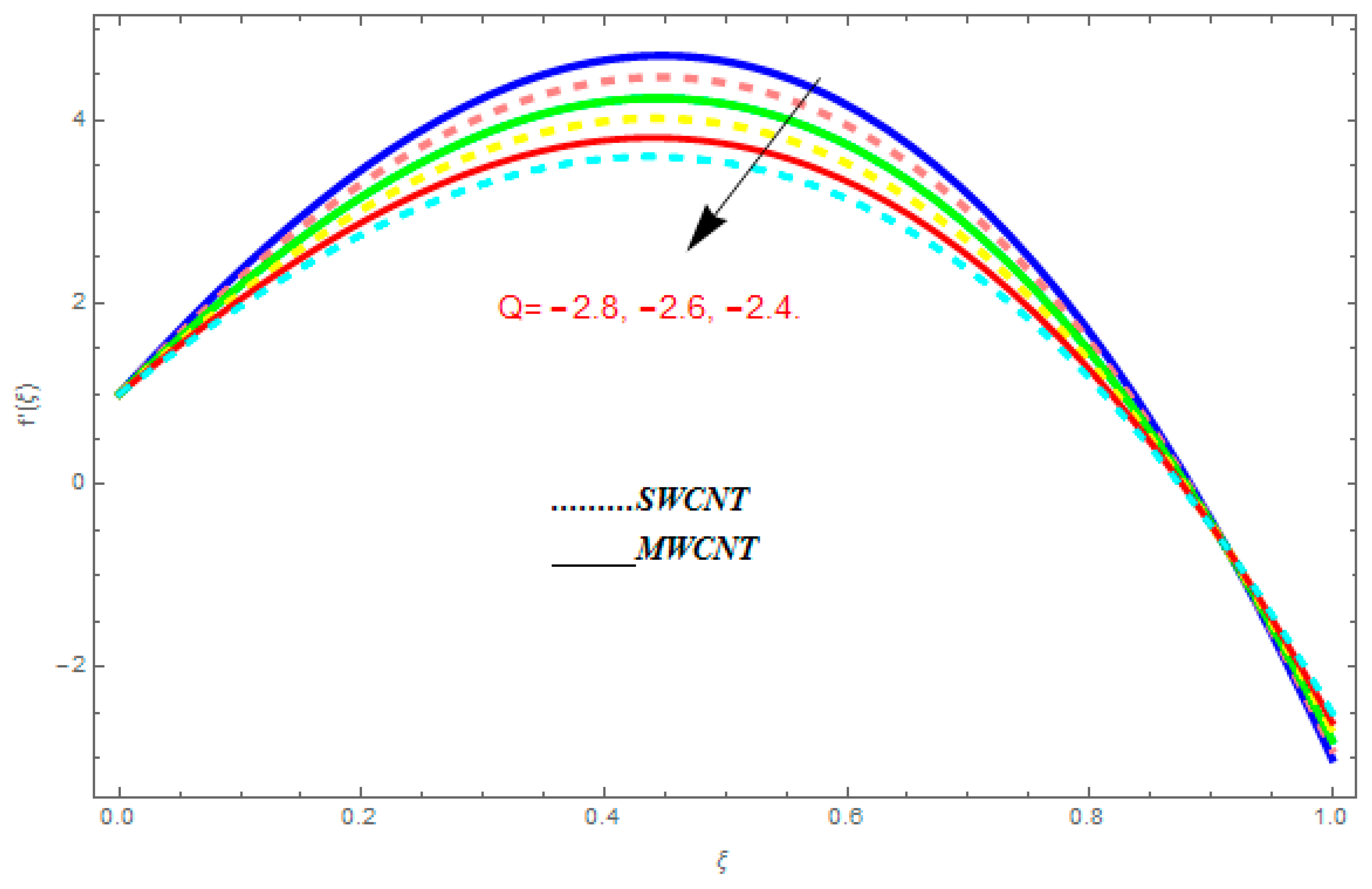
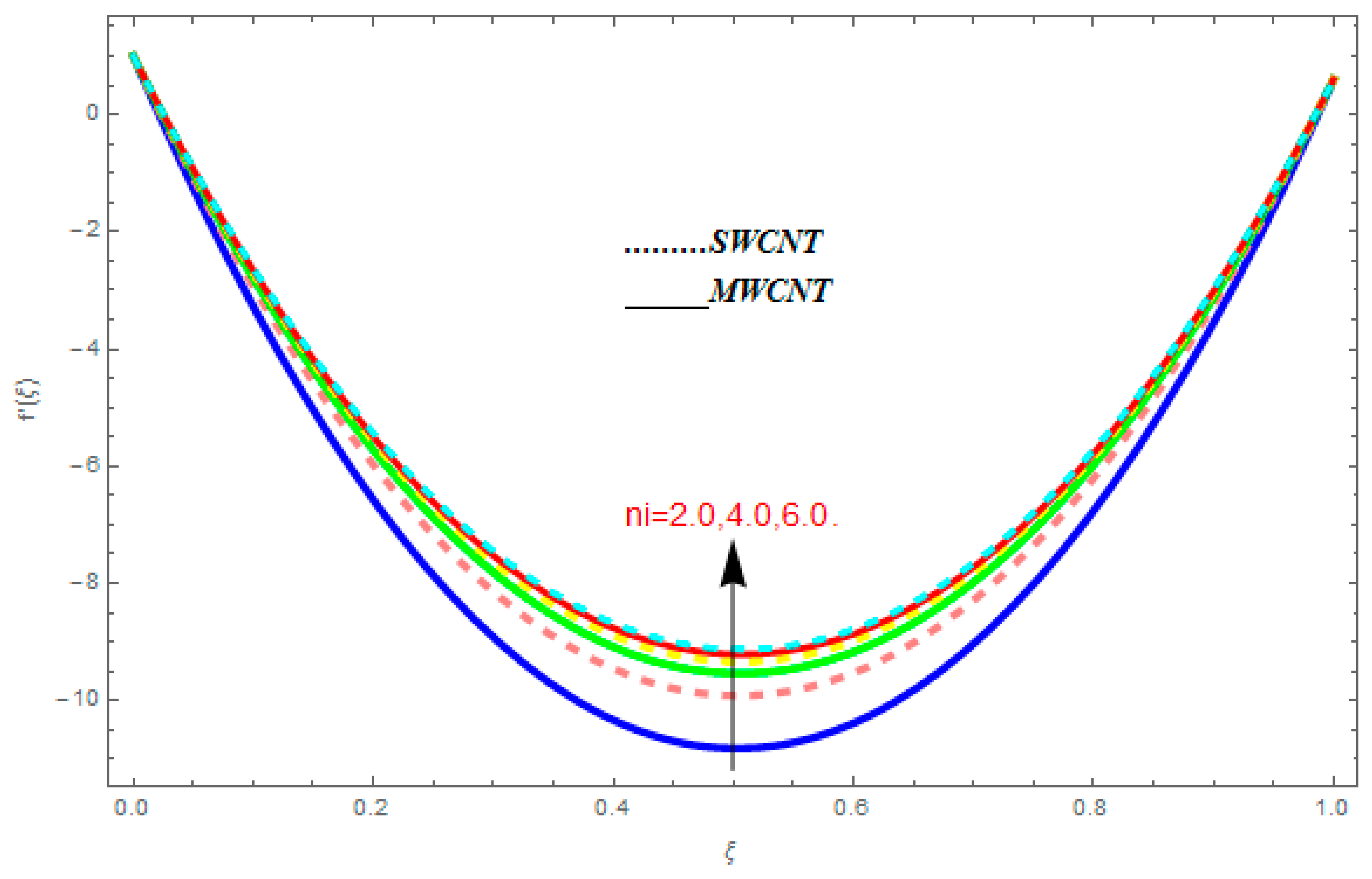
- The velocity function increased with the augmentation in , positive , , and , while it reduced with higher values of , , , and negative .
- (b)
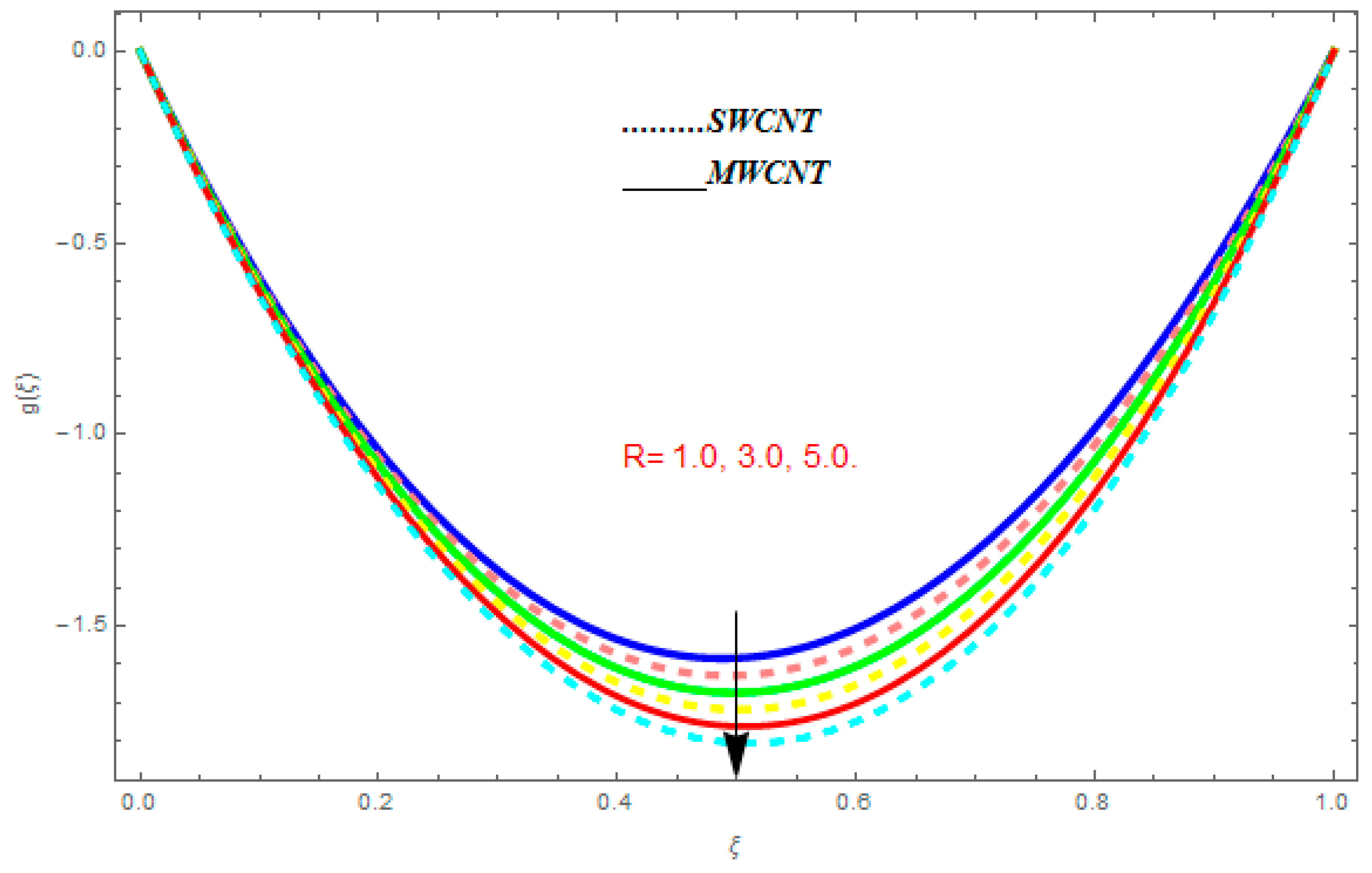
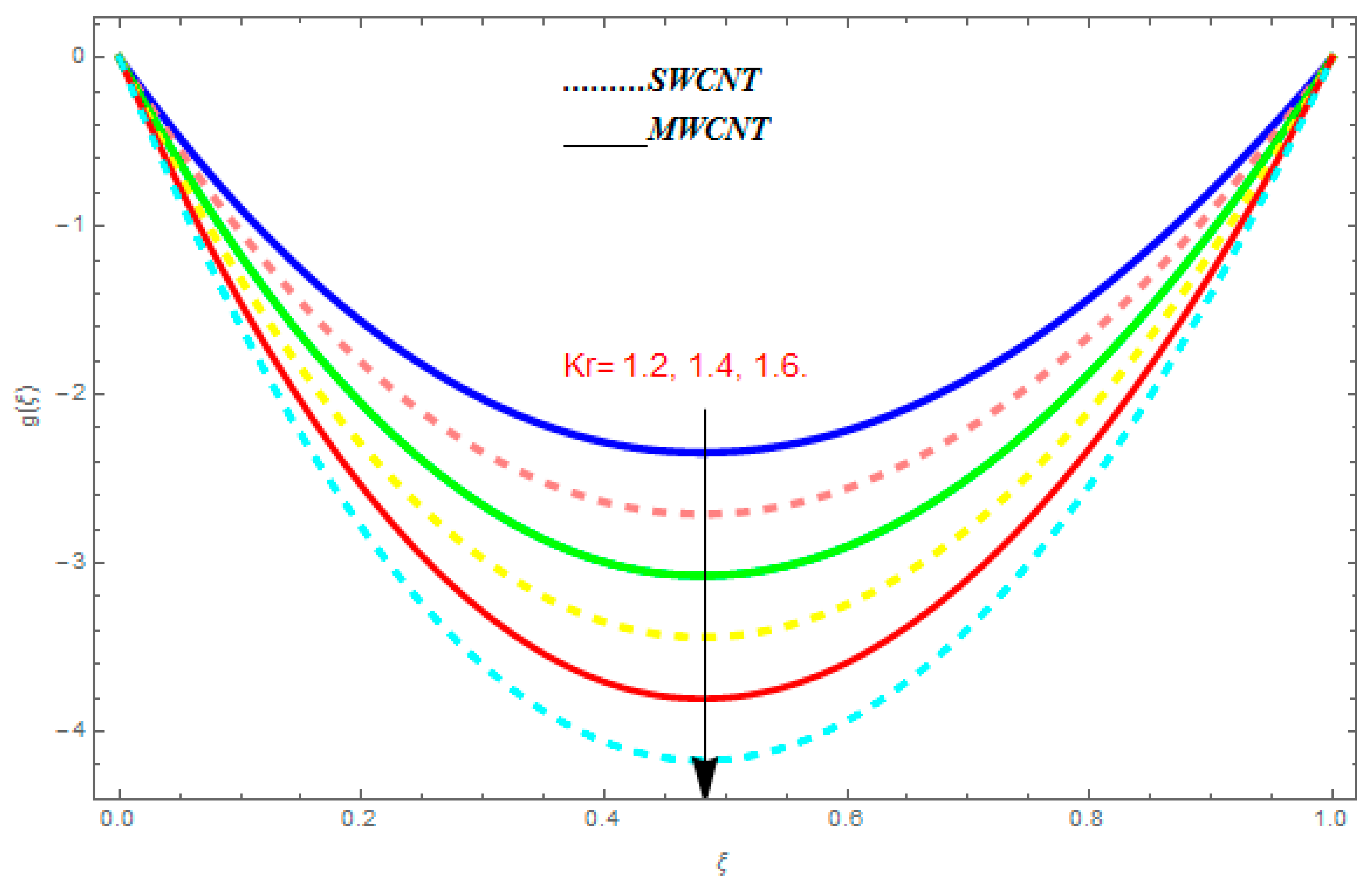
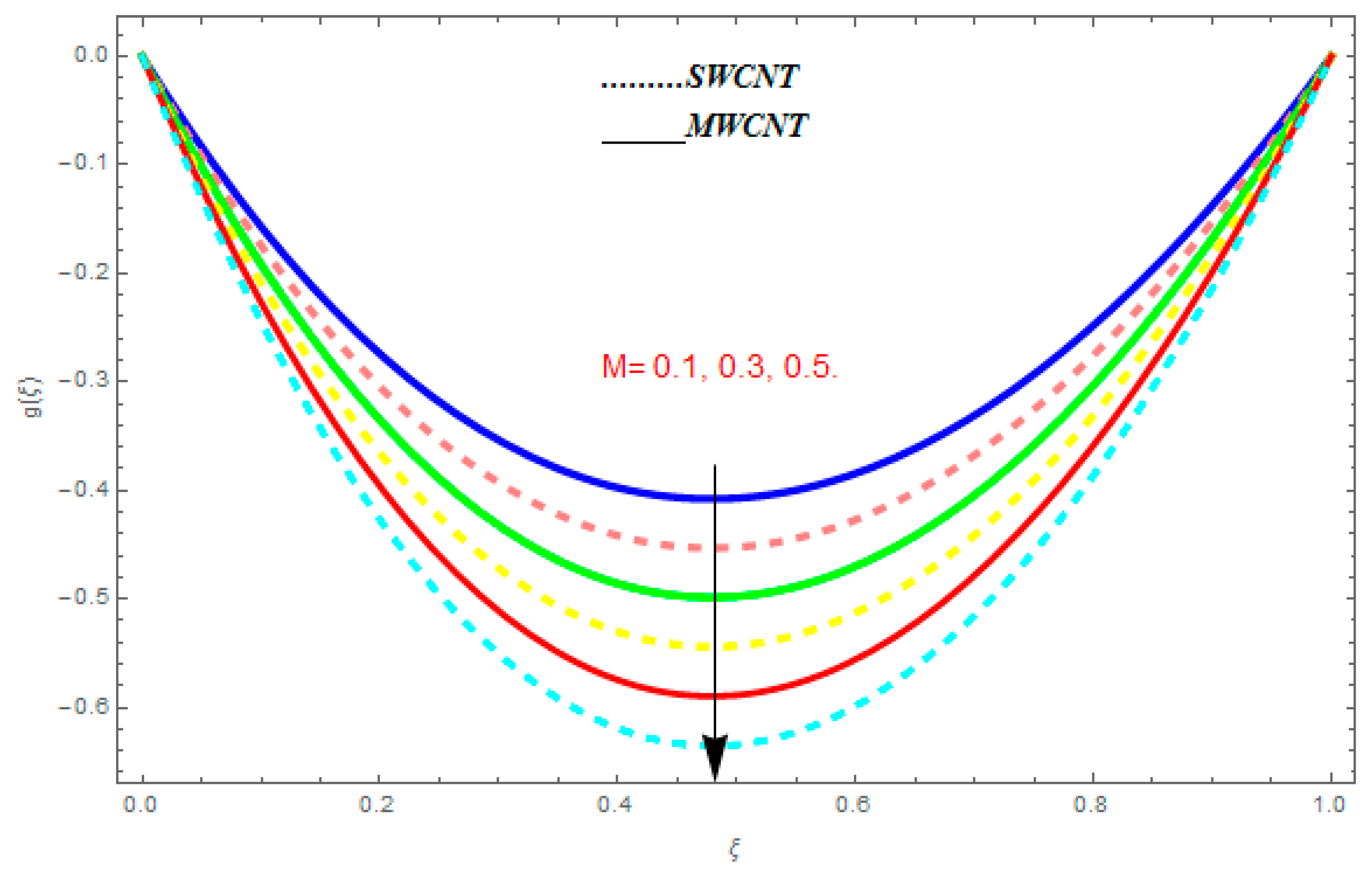
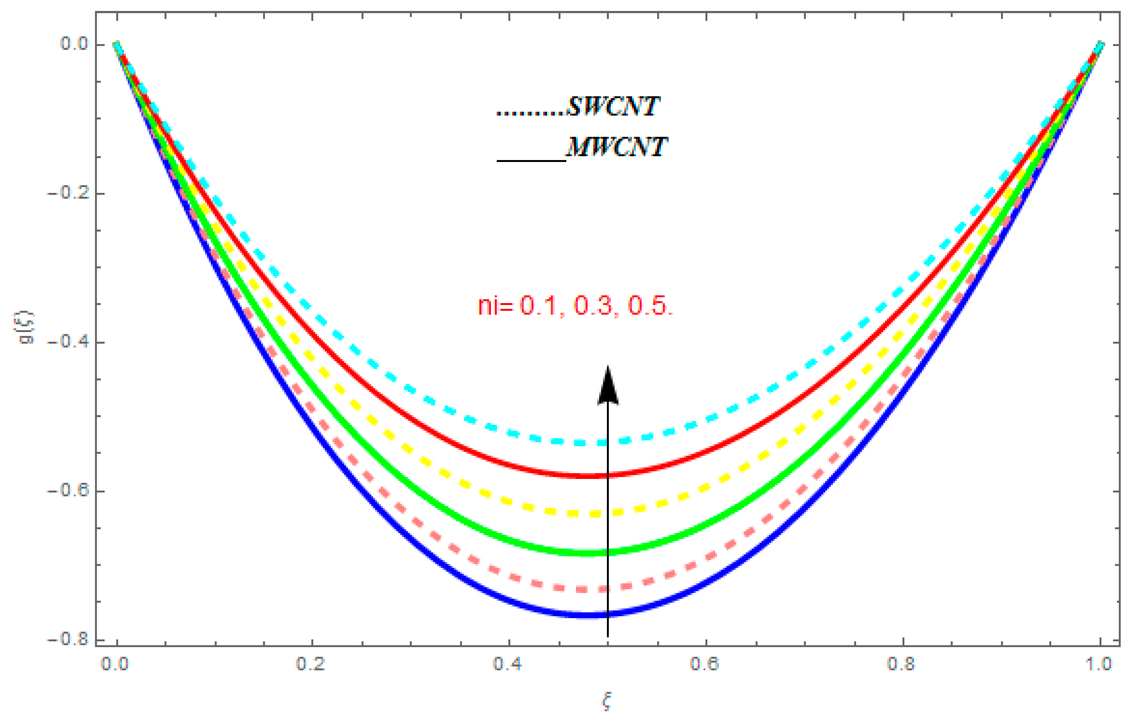
- It is observed that the transverse velocity function increased with greater value of , while it showed a reducing behavior for higher values of , , and .
- (c)
- The temperature function was augmented with the augmentation in , while it showed reducing behavior with the escalation in .
- (d)
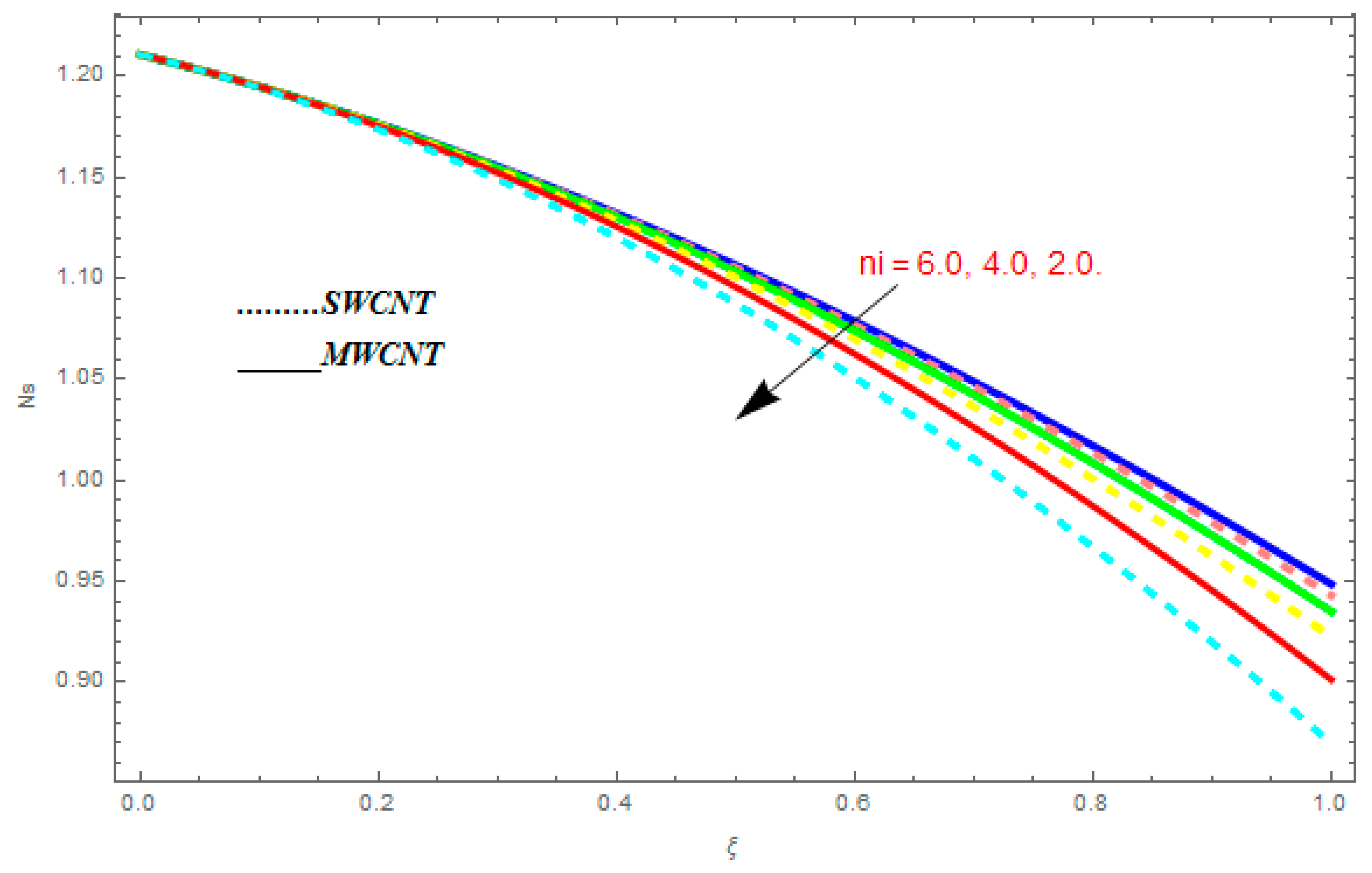
- For entropy profile, it was observed that entropy generation increased with higher value of while it showed decreasing behavior with an increase in .
- (e)
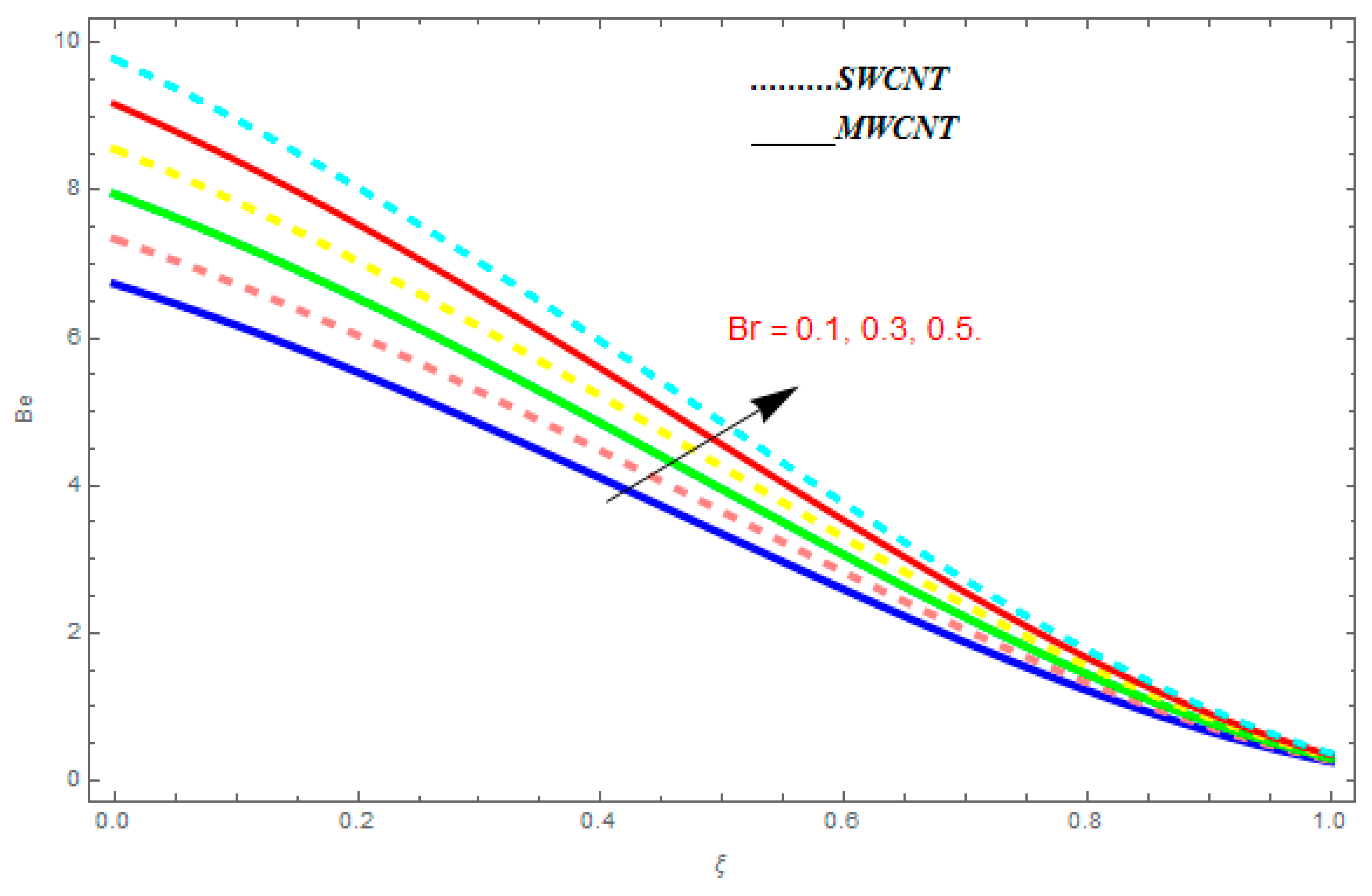
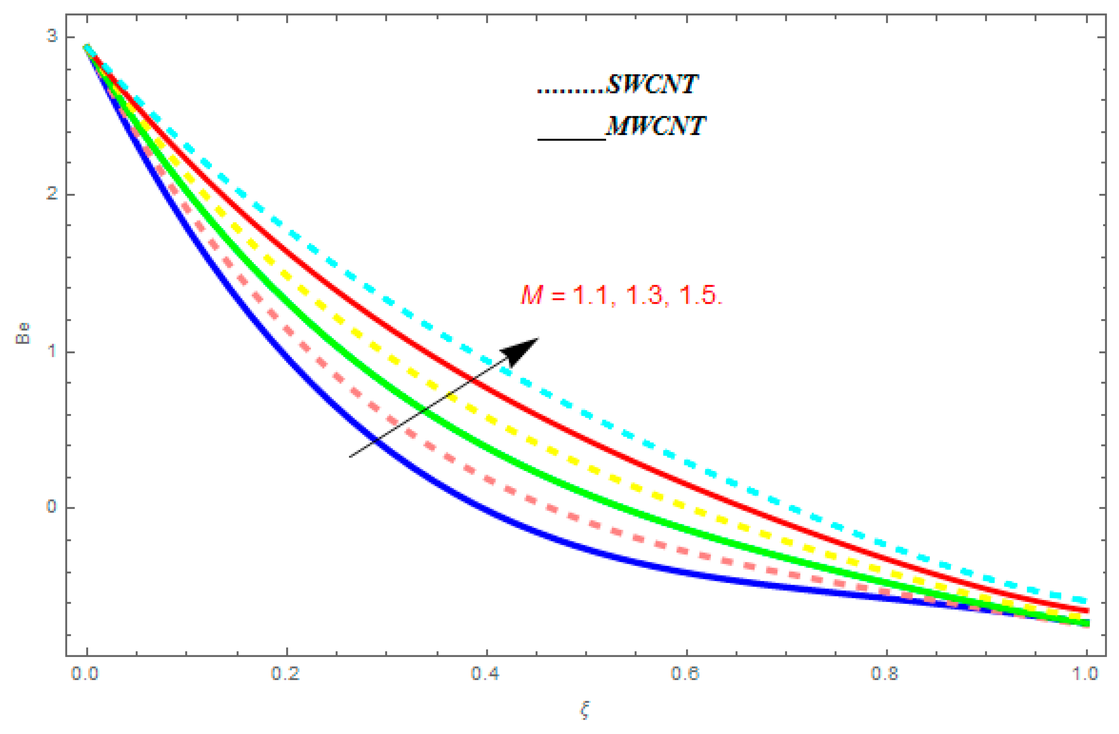
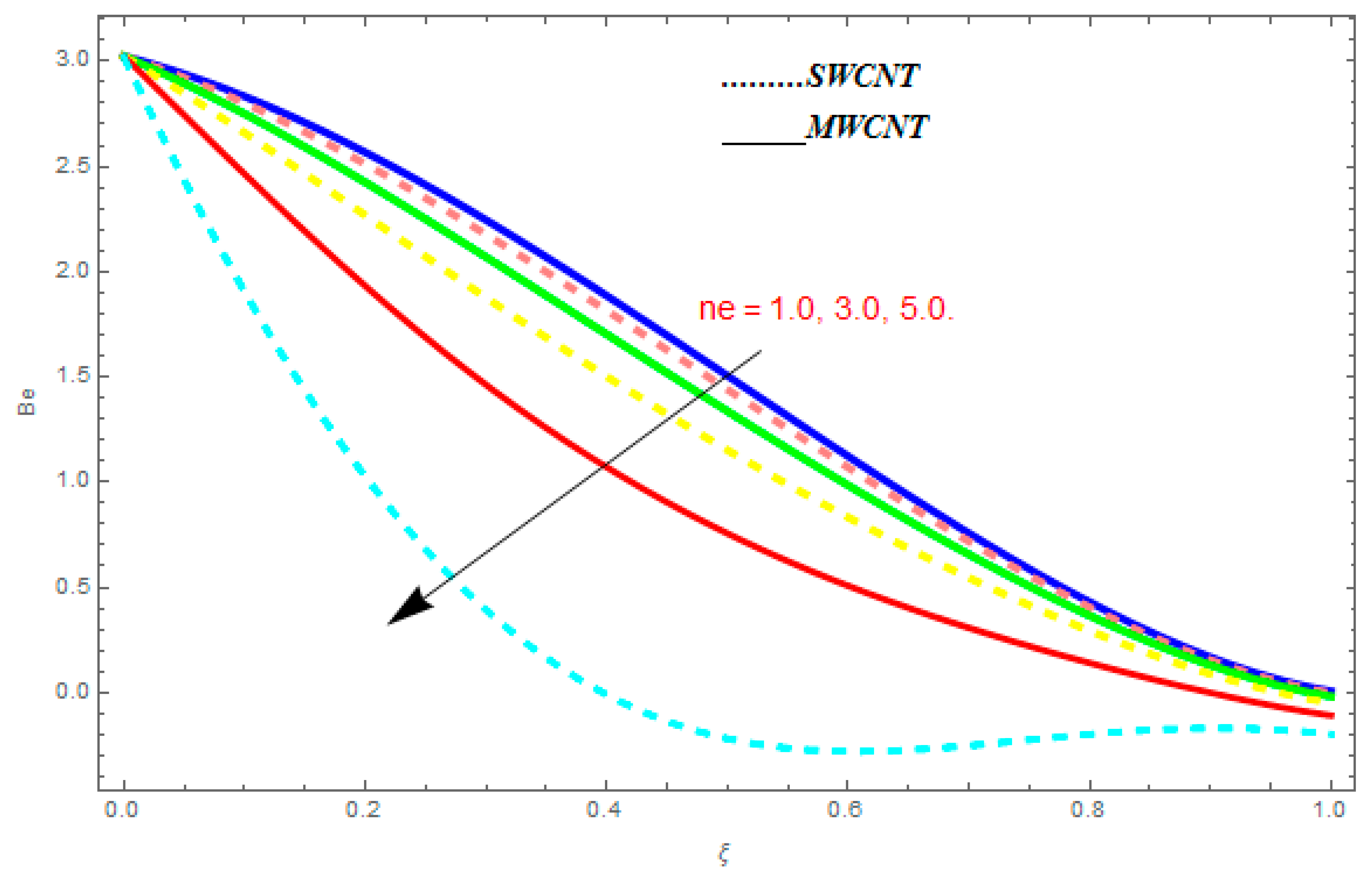
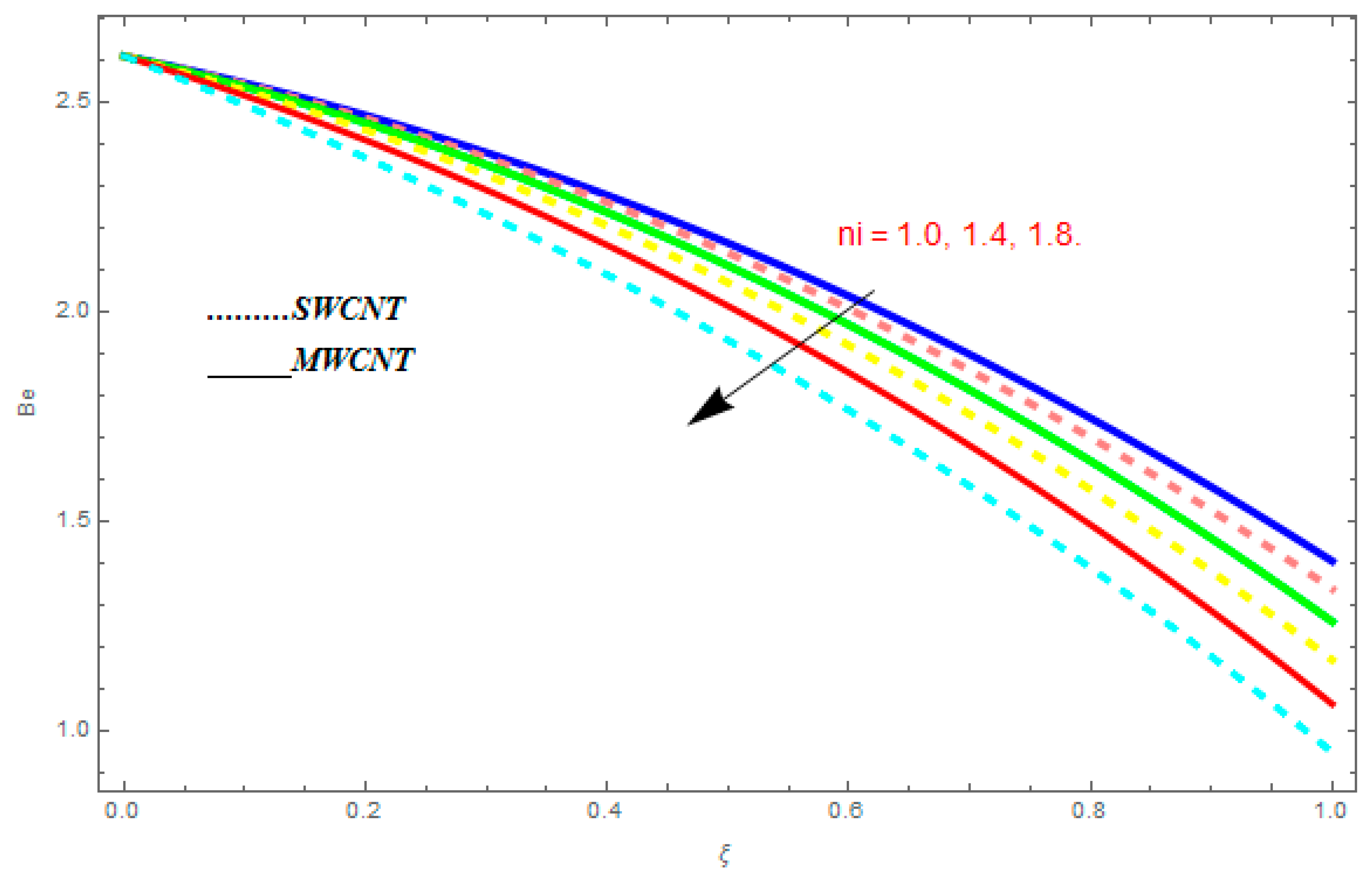
- The Bejan number showed increasing behavior with an increase in , , while it showed decreasing behavior with an increase in .
Author Contributions
Acknowledgments
Conflicts of Interest
Nomenclature
| Pr | Prandtl number | similarity variables | |
| P | fluid pressure | surface shear stress | |
| Nusselt number | electrical conductivity | ||
| internal energy distribution functions | thermal diffusivity | ||
| magnetic flux density | τ | lattice relaxation time | |
| Bejan number. | volume friction | ||
| Hall parameter | thermal conductivity | ||
| magnetic parameter | thermal diffusivity | ||
| current density | angular velocity | ||
| electric intensity | dynamic viscosity | ||
| ion-slip parameter | electron cyclotron | ||
| a, b, c | constants | ||
| fluid temperature | Subscripts | ||
| specific heat | nanofluid | ||
| carbon nanotubes | |||
| skin friction coefficient | hot | ||
| Reynolds number | average | ||
| suction and injection | |||
| rotation parameter | |||
| distance between the plates | |||
| surface heat flux | |||
| Dimensional entropy generation | |||
| non-dimensional entropy generation | |||
| , | velocities components | ||
| coordinates | |||
| origin | |||
| Nusselt number | |||
| Greek symbols | |||
| kinematic viscosity | |||
| fluid density | |||
References
- Xiao, B.; Chen, H.; Xiao, S.; Cai, J. Research on Relative Permeability of Nanofibers with Capillary Pressure Effect by Means of Fractal-Monte Carlo Technique. J. Nanosci. Nanotechnol. 2017, 17, 6811–6817. [Google Scholar] [CrossRef]
- Xiao, B.; Wang, W.; Fan, J.; Chen, H.; Hu, X.; Zhao, D.; Zhang, X.; Ren, W. Optimization of the Fractal-Like Architecture of Porous Fibrous Materials Related to Permeability, Diffusivity and Thermal Conductivity. Fractals 2017. [Google Scholar] [CrossRef]
- Xiao, B.; Zhang, X.; Wang, W.; Long, G.; Chen, H.; Kang, H.; Ren, W. A fractal model for water flow through unsaturated porous rocks. Fractals 2018. [Google Scholar] [CrossRef]
- Liang, M.; Liu, Y.; Xiao, B.; Yang, S.; Han, H. An analytical model for the transverse permeability of gas diffusion layer with electrical double layer effects in proton exchange membrane fuel cells. Int. J. Hydrog. Energy 2018. [Google Scholar] [CrossRef]
- Long, G.; Xu, G. The Effects of Perforation Erosion on Practical Hydraulic-Fracturing Applications. SPE J. 2017, 22, 645–659. [Google Scholar] [CrossRef]
- Long, G.; Liu, S.; Xu, G.; Wong, S.W.; Chen, H.; Xiao, B. A Perforation-Erosion Model for Hydraulic-Fracturing Applications. SPE Prod. Oper. 2018, 33, 770–783. [Google Scholar] [CrossRef]
- Kroto, H.W.; Heath, J.R.; O’Brien, S.C.; Curl, R.F.; Smalley, R.E. C60: The Best Constant of Discrete Sobolev Inequality on a Weighted Truncated Tetrahedron. Buckminsterfullerene. Nature 1985, 318, 162–163. [Google Scholar] [CrossRef]
- Iijima, S. Helical microtubules of graphitic carbon. Nature 1991, 354, 56–58. [Google Scholar] [CrossRef]
- Muhammad, S.; Ali, G.; Shah, Z.; Islam, S.; Hussain, A. The Rotating Flow of Magneto Hydrodynamic Carbon Nanotubes over a Stretching Sheet with the Impact of Non-Linear Thermal Radiation and Heat Generation/Absorption. Appl. Sci. 2018, 8, 482. [Google Scholar] [CrossRef]
- Novoselov, K.S.; Geim, A.K.; Morozov, S.V.; Jiang, D.; Zhang, Y.; Dubonos, S.V. Electric field effect in atomically thin carbon films. Science 2004, 306, 666–669. [Google Scholar] [CrossRef] [PubMed]
- Casari, C.S.; Tommasini, M.; Tykwinski, R.R.; Milani, A. Carbon-atom wires 1-D systems with tunable properties. Nanoscale 2016, 8, 4414–4435. [Google Scholar] [CrossRef] [PubMed]
- Choi, S.U.S. Enhancing thermal conductivity of fluids with nanoparticles. In Proceedings of the 1995 ASME International Mechanical Engineering Congress and Exposition, San Francisco, CA, USA, 12–17 November 1995; pp. 99–105. [Google Scholar]
- Kang, H.U.; Kim, S.H.; Oh, J.M. Estimation of thermal conductivity of nanofluid using experimental effective particle volume. Exp. Heat Transf. 2006, 19, 181–191. [Google Scholar] [CrossRef]
- Haq, R.U.; Nadeem, S.; Khan, Z.H.; Noor, N.F.M. Convective heat transfer in MHD slips flow over a stretching surface in the presence of carbon nanotubes. Phys. B Condens. Matter 2015, 457, 40–47. [Google Scholar] [CrossRef]
- Liu, M.S.; Lin, M.C.C.; Te, H.I.; Wang, C.C. Enhancement of thermal conductivity with carbon nanotube for nanofluids. Int. Commun. Heat Mass Transf. 2005, 32, 1202–1210. [Google Scholar] [CrossRef]
- Shah, Z.; Dawar, A.; Islam, S.; Khan, I.; Ching, D.L.C. Darcy-Forchheimer Flow of Radiative Carbon Nanotubes with Microstructure and Inertial Characteristics in the Rotating Frame. Case Stud. Eng. 2018. [Google Scholar] [CrossRef]
- Alrashed, A.A.A.A.; Gharibdousti, M.S.; Goodarzi, M.; Oliveira, L.R.; Filho, E.P. Effects on thermophysical properties of carbon based nanofluids: Experimental data, modelling using regression, ANFIS and ANN. Int. J. Heat Mass Transf. 2018, 23, 920–932. [Google Scholar] [CrossRef]
- Safaei, M.R.; Togun, K.H.; Vafai, S.; Kazi, N.; Badarudin, A. Investigation of Heat Transfer Enhancement in a Forward-Facing Contracting Channel Using FMWCNT Nanofluids. Int. J. Comput. Methodol. 2014. [Google Scholar] [CrossRef]
- Khan, W.; Gul, T.; Idrees, M.; Islam, S.; Khan, I.; Dennis, L.C.C. Thin Film Williamson Nanofluid Flow with Varying Viscosity and Thermal Conductivity on a Time-Dependent Stretching Sheet. Appl. Sci. 2016, 6, 334. [Google Scholar] [CrossRef]
- Sheikholeslami, M.; Hatami, D.; Ganji, D.D. Nanofluid flow and heat transfer in a rotating system in the presence of a magnetic field. J. Mol. Liq. 2014, 190, 112–120. [Google Scholar] [CrossRef]
- Sheikholeslami, M. Lattice Boltzmann Method simulation of MHD non-Darcy nanofluid free convection. Physica B 2017, 516, 55–71. [Google Scholar] [CrossRef]
- Sheikholeslami, M. Influence of magnetic field on nanofluid free convection in an open porous cavity by means of Lattice Boltzmann Method. J. Mol. Liq. 2017, 234, 364–374. [Google Scholar] [CrossRef]
- Sheikholeslami, M. Magnetohydrodynamic nanofluid forced convection in a porous lid driven cubic cavity using Lattice Boltzmann Method. J. Mol. Liq. 2017, 231, 555–565. [Google Scholar] [CrossRef]
- Jawad, M.; Shah, Z.; Islam, S.; Islam, S.; Bonyah, E.; Khan, Z.A. Darcy-Forchheimer flow of MHD nanofluid thin film flow with Joule dissipation and Navier’s partial slip. J. Phys. Commun. 2018. [Google Scholar] [CrossRef]
- Khan, N.; Zuhra, S.; Shah, Z.; Bonyah, E.; Khan, W.; Islam, S. Slip flow of Eyring-Powell nanoliquid film containing graphene nanoparticles. AIP Adv. 2018, 8, 115302. [Google Scholar] [CrossRef]
- Khan, A.S.; Nie, Y.; Shah, Z.; Dawar, A.; Khan, W.; Islam, S. Three-Dimensional Nanofluid Flow with Heat and Mass Transfer Analysis over a Linear Stretching Surface with Convective Boundary Conditions. Appl. Sci. 2018, 8, 2244. [Google Scholar] [CrossRef]
- Mendoza, E. Reflections on the Motive Power of Fire and other Papers on the Second Law of Thermodynamics; Clapeyron, E., Clausius, R., Eds.; Dover Publications: New York, NY, USA, 1988; ISBN 0-486-44641-7. [Google Scholar]
- Clausius, R. Mechanical Theory of Heat; Institute of Human Thermodynamics Publishing Ltd.: Chicago, IL, USA, 2006; pp. 1850–1865. [Google Scholar]
- Bejan, A. Second law analysis in heat transfer. Energy 1980, 5, 720–732. [Google Scholar] [CrossRef]
- Rashidi, M.M.; Kavyani, N.; Abelman, S. Investigation of entropy generation in MHD and slip flow over a rotating porous disk with variable. Int. J. Heat Mass Transf. 2014, 70, 892–917. [Google Scholar] [CrossRef]
- Soomro, F.A.; Rizwan-ul-Haq, K.Z.H.; Zhang, Q. Numerical study of entropy generation in MHD water-based carbon nanotubes along an inclined permeable surface. Eur. Phys. J. Plus 2017, 132, 412. [Google Scholar] [CrossRef]
- Mohammad, I.; Gohar, A.; Shah, Z.; Islam, S.; Muhammad, S. Entropy Generation on Nanofluid Thin Film Flow of Eyring–Powell Fluid with Thermal Radiation and MHD Effect on an Unsteady Porous Stretching Sheet. Entropy 2018, 20, 412. [Google Scholar] [CrossRef]
- Darbari, B.; Rashidi, S.; Esfahani, J.A. Sensitivity analysis of entropy generation in nanofluid flow inside a channel by response surface methodology. Entropy 2016, 18, 52. [Google Scholar] [CrossRef]
- Bhatti, M.M.; Abbas, T.; Mehdi, M.; Rashidi, M.; Mohamed, S.; Ali, E. Numerical simulation of Entropy Generation with thermal radiation on MHD Carreau Nanofluid towards a Shrinking Sheet. Entropy 2016, 18, 200. [Google Scholar] [CrossRef]
- Mohammad, Y.A.J.; Mohammad, R.S.; Abdullah, A.; Truong, K.N.; Enio, P.B.F. Entropy Generation in Thermal Radiative Loading of Structures with Distinct Heaters. Entropy 2017, 19, 506. [Google Scholar] [CrossRef]
- Mohammad, M.R.; Mohammad, N.; Mustafa, S.S.; Zhighang, Y. Entropy Generation in a Circular Tube Heat Exchanger Using Nanofluids: Effects of Different Modeling Approaches. J. Heat Transf. Eng. 2017. [Google Scholar] [CrossRef]
- Cramer, K.; Pai, S. Magnetofluid Dynamics for Engineers and Applied Physicists; McGraw-Hill: New York, NY, USA, 1973. [Google Scholar]
- Attia, H.A. Effect of the ion slip on the MHD flow of a dusty fluid with heat transfer under exponential decaying pressure gradient. Cent. Eur. J. Phys. 2005, 3, 484–507. [Google Scholar] [CrossRef] [Green Version]
- Motsa, S.S.; Shatery, S. The effects of chemical reaction, Hall and ion-slip currents on MHD micropolar fluid flow with thermal diffusivity using a noval numerical technique. J. Appl. Math. 2012. [Google Scholar] [CrossRef]
- Shah, Z.; Islam, S.; Ayaz, H.; Khan, S. Radiative Heat and Mass Transfer Analysis of Micropolar Nanofluid Flow of Casson Fluid between Two Rotating Parallel Plates with Effects of Hall Current. ASME J. Heat Transf. 2018. [Google Scholar] [CrossRef]
- Shah, Z.; Islam, S.; Gul, T.; Bonyah, E.; Altaf Khan, M. The Elcerical MHD And Hall Current Impact On Micropolar Nanofluid Flow Between Rotating Parallel Plates. Results Phys. 2018. [Google Scholar] [CrossRef]
- Greenspan, H.P.; Howard, L.N. On a time-dependent motion of a rotating fluid. J. Fluid Mech. 1963, 17, 385–404. [Google Scholar] [CrossRef]
- Nazar, R.; Amin, N.; Pop, I. Unsteady boundary layer flow due to a stretching surface in a rotating fluid. Mech. Res. Commun. 2004, 31, 121–128. [Google Scholar] [CrossRef]
- Mustafa, M.; Wasim, M.; Hayat, T.; Alsaedi, A. A revised model to study the rotating flow of nanofluid over an exponentially deforming sheet: Numerical solutions. J. Mol. Liq. 2017, 225, 320–327. [Google Scholar] [CrossRef]
- Khan, A.; Shah, Z.; Islam, S.; Khan, S.; Khan, W.; Khan, Z.A. Darcy–Forchheimer flow of micropolar nanofluid between two plates in the rotating frame with non-uniform heat generation/absorption. Adv. Mech. Eng. 2018. [Google Scholar] [CrossRef]
- Nor AthirahMohd, Z.; Khan, I.; Sharidan, S.; Alshomrani, A.S. Analysis of heat transfer for unsteady MHD free convection flow of rotating Jeffrey nanofluid saturated in a porous medium. Results Phys. 2017, 7, 288–309. [Google Scholar] [CrossRef]
- Mohammadreza, H.; Rad, S.; Goodarz, A.; Mahidzal, B.D.; Salim, N.K.; Mohammad, R.S.; Emad, S. Numerical Study of Entropy Generation in a Flowing Nanofluid Used in Micro- and Minichannels. Entropy 2013, 15, 144–155. [Google Scholar] [CrossRef] [Green Version]
- Nasiri, H.; Jamalabadi, M.Y.A.; Safaei, M.R.; Nguyen, T.K.; Shadlo, M.S. A smoothed particle hydrodynamics approach for numerical simulation of nano-fluid flows. J. Therm. Anal. 2018. [Google Scholar] [CrossRef]
- Bhatti, M.M.; Sheikhulislami, M.; Zeeshan, A. Entropy Analysis on Electro-Kinetically Modulated Peristaltic Propulsion of Magnetized Nanofluid Flow through a Microchannel. Entropy 2017, 19, 481. [Google Scholar] [CrossRef]
- Yarmand, H.; Ahmadi, G.; Gharehkhani, G.; Kazi, S.N.; Safei, M.R.; Alehshem, M.S.; Mahat, A.B. Entropy Generation during Turbulent Flow of Zirconia-water and Other Nanofluids in a Square Cross Section Tube with a Constant Heat Flux. Entropy 2014, 16, 6116–6132. [Google Scholar] [CrossRef] [Green Version]
- Cho, C.C.; Yau, H.T.; Chiu, C.H.; Chiu, K.C. Numerical Investigation into Natural Convection and Entropy Generation in a Nanofluid-Filled U-Shaped Cavity. Entropy 2015, 17, 5980–5994. [Google Scholar] [CrossRef] [Green Version]
- Shadlo, M.S.; kimiaeifar, A.; Bagheri, D. Series solution for heat transfer of continuous stretching sheet immersed in a micropolar fluid in the existence of radiation. Int. J. Numer. Methods Heat Fluid Flow 2013, 23, 289–304. [Google Scholar] [CrossRef]
- Aghaei, A.; Sheikhzadeh, G.A.; Goodarzi, M.; Hasani, H.; Damirchi, H.; Afrand, M. Effect of horizontal and vertical elliptic baffles inside an enclosure on the mixed convection of a MWCNTs-water nanofluid and its entropy generation. Eur. Phys. J. Plus 2018, 133, 486. [Google Scholar] [CrossRef]
- Liao, S.J. On the Analytic Solution of Magnetohydrodynamic Flows of Non-Newtonian Fluids over a Stretching Sheet. J. Fluid Mech. 2013, 488, 189–212. [Google Scholar] [CrossRef]
- Liao, S.J. On Homotopy Analysis Method for Nonlinear Problems. Appl. Math. Comput. 2004, 147, 499–513. [Google Scholar] [CrossRef]
- Shah, Z.; Bonyah, E.; Islam, S.; Khan, W.; Ishaq, M. Radiative MHD thin film flow of Williamson fluid over an unsteady permeable stretching. Heliyon 2018, 4, e00825. [Google Scholar] [CrossRef]
- Hammed, K.; Haneef, M.; Shah, Z.; Islam, I.; Khan, W.; Asif, S.M. The Combined Magneto hydrodynamic and electric field effect on an unsteady Maxwell nanofluid Flow over a Stretching Surface under the Influence of Variable Heat and Thermal Radiation. Appl. Sci. 2018, 8, 160. [Google Scholar] [CrossRef]
- Shadlo, M.S.; Kimiaeifar, A. Application of homotopy perturbation method to find an analytical solution for magnetohydrodynamic flows of viscoelastic fluids in converging/diverging channels. J. Mech. Eng. Sci. Part C 2010. [Google Scholar] [CrossRef]
- Maxwell, J.C. Electricity and Magnetism, 3rd ed.; Clarendon: Oxford, UK, 1904. [Google Scholar]
- Jaffery, D.J. Conduction through a random suspension of spheres. Proc. R. Soc. Lond. Ser. A Math. Phys. Sci. 1973, 335, 335–336. [Google Scholar] [CrossRef]
- Davis, R. The effective thermal conductivity of a composite material with spherical inclusions. Int. J. 1986, 7, 609–620. [Google Scholar] [CrossRef]
- Hamilton, R.L.; Crosser, O.K. Thermal conductivity of heterogenous two-component systems. Ind. Eng. Chem. Fund. 1962, 3, 187–191. [Google Scholar] [CrossRef]
- Xue, Q. Model for thermal conductivity of carbon nanotube-based composites. Phys. B Condens. Matter 2005, 368, 302–307. [Google Scholar] [CrossRef]


| at | at | ||||||
|---|---|---|---|---|---|---|---|
| 0.1 | 0.2 | 0.4 | 0.5 | 0.3 | 0.2 | −0.484638 | −0.515879 |
| 0.3 | −0.470976 | −0.529161 | |||||
| 0.5 | 0.2 | −0.458474 | −0.541466 | ||||
| 0.4 | −0.461839 | −0.538401 | |||||
| 0.6 | 0.4 | −0.465886 | −0.534719 | ||||
| 0.7 | −0.472578 | −0.529764 | |||||
| 1.0 | −1.5 | −0.483196 | −0.521086 | ||||
| −0.1 | −2.187070 | −1.202060 | |||||
| 0.1 | −1.006670 | −0.971885 | |||||
| 1.5 | 0.3 | −0.835078 | 0.523539 | ||||
| 0.4 | 0.491335 | 0.511560 | |||||
| 0.5 | 0.2 | 0.498996 | −0.503849 | ||||
| 0.6 | 0.490763 | 0.511484 | |||||
| 1.0 | 0.495080 | 0.507058 |
| at | at | |||||||
|---|---|---|---|---|---|---|---|---|
| 0.1 | 0.2 | 0.4 | 0.5 | 0.3 | 0.2 | 7.2 | −0.001105 | 0.000884 |
| 0.3 | −0.001107 | 0.000886 | ||||||
| 0.5 | 0.2 | −0.001110 | 0.000889 | |||||
| 0.4 | −0.001445 | 0.001157 | ||||||
| 0.6 | 0.4 | −0.001779 | 0.001429 | |||||
| 0.7 | −0.002337 | 0.001887 | ||||||
| 1.0 | −1.5 | −0.002932 | 0.002347 | |||||
| −0.1 | −0.000808 | 0.000995 | ||||||
| 0.1 | −0.002280 | 0.001443 | ||||||
| 1.5 | 0.3 | −0.002596 | 0.004649 | |||||
| 0.4 | −0.003721 | 0.004249 | ||||||
| 0.5 | 0.2 | −0.003404 | 0.003887 | |||||
| 0.6 | −0.002348 | 0.002682 | ||||||
| 1.0 | 7.2 | −0.001862 | 0.002126 | |||||
| 7.3 | −0.001862 | 0.002126 | ||||||
| 7.5 | −0.001862 | 0.002126 |
| Materials | SWCNTs | MWCNTs |
|---|---|---|
| Thermal Conductivity () | 3000 | 3000 |
| Specific gravity (g/cm3) | ||
| Strength | 50–500 | 10–60 |
| Elastic Modulus | 1 | 0.3–1 |
© 2019 by the authors. Licensee MDPI, Basel, Switzerland. This article is an open access article distributed under the terms and conditions of the Creative Commons Attribution (CC BY) license (http://creativecommons.org/licenses/by/4.0/).
Share and Cite
Feroz, N.; Shah, Z.; Islam, S.; Alzahrani, E.O.; Khan, W. Entropy Generation of Carbon Nanotubes Flow in a Rotating Channel with Hall and Ion-Slip Effect Using Effective Thermal Conductivity Model. Entropy 2019, 21, 52. https://doi.org/10.3390/e21010052
Feroz N, Shah Z, Islam S, Alzahrani EO, Khan W. Entropy Generation of Carbon Nanotubes Flow in a Rotating Channel with Hall and Ion-Slip Effect Using Effective Thermal Conductivity Model. Entropy. 2019; 21(1):52. https://doi.org/10.3390/e21010052
Chicago/Turabian StyleFeroz, Nosheen, Zahir Shah, Saeed Islam, Ebraheem O. Alzahrani, and Waris Khan. 2019. "Entropy Generation of Carbon Nanotubes Flow in a Rotating Channel with Hall and Ion-Slip Effect Using Effective Thermal Conductivity Model" Entropy 21, no. 1: 52. https://doi.org/10.3390/e21010052