1. Introduction
In the
M-closed world, where a fitted model class is implicitly assumed to contain the sample distribution from which the data came, Bayesian updating is highly compelling. However, modern statisticians are increasingly acknowledging that their inference is taking place in the
M-open world [
1]. Within this framework we acknowledge that any class of models we choose is unlikely to capture the actual sampling distribution, and is then at best an approximate description of our own beliefs and the underlying real world process. In this situation it is no longer possible to learn about the parameter which generated the data and a statistical divergence measure must be specified between the fitted model and the genuine one in order to define the parameter targeted by the inference [
2]. Remarkably in the
M-open world, standard Bayesian updating can be seen as a method which learns a model by minimising the predictive Kullback–Leibler (KL)-divergence from the model from which the data were sampled [
2,
3]. Therefore, traditional Bayesian updating turns out to still be a well principled method for belief updating provided the decision maker (DM) concerns themselves with the parameter of the model that is closest to the data as measured by KL-divergence [
2]. Recall the KL-divergence of functioning model
f from data generating density
g is defined as the extra logarithmic score incurred for believing
Z was distributed according to
F when it was actually distributed according to
G [
1]
It is well known that when the KL-divergence is large, which is almost inevitable in high dimensional problems, the KL-divergence minimising models can give a very poor approximation if our main interest is in getting the central part of the posterior model uncertainty well estimated. This is because the KL-divergence gives large consideration to correctly specifying the tails of the generating sample distribution—see
Section 2.2.1. As a result, when the DM acknowledges that they are in the
M-open world, they have several options currently available to them:
- 1.
Proceed as though the model class does contain the true sample distribution and conduct a posteriori sensitivity analysis.
- 2.
Modify the model class in order to improve its robustness properties.
- 3.
Abandon the given parametric class and appeal to more data driven techniques.
To this we add:
- 4.
Acknowledge that the model class is only approximate, but is the best available, and seek to infer the model parameters in a way that are most useful to the decision maker.
Method 1 is how [
4] recommends approaching parametric model estimation and is the most popular approach amongst statisticians. Although it is acknowledged that the model is only approximate, Bayesian inference is applied as though the statistician believes the model to be correct. The results are then checked to examine how sensitive these are to the approximations made. Authors [
5] provide a thorough review while [
6] consider this in a decision focused manner.
Method 2 corresponds to the classical robustness approach. Within this approach, one model within the parametric class may be substituted for a model providing heavier tails [
5]. Alternatively, different estimators, for example M-estimators [
7,
8], see [
9] for a Bayesian analogue, are used instead of those justified by the model class. Bayes linear methods [
10], requiring many fewer belief statements than a full probability specification, form a special subclass of these techniques.
The third possibility is to abandon any parametric description of the probability space. Examples of this solution include, empirical likelihood methods [
11]; a decision focused general Bayesian update [
3]; Bayesian non-parametric methods; or to appeal to statistical learning methods such as neural networks or support vector machines. Such methods simply substitute the assumptions and structure associated with the model class, for a much broader class of models with less transparent assumptions and thus are not as free of misspecification related worries as they may seem.
Though alternatives 2 and 3 can be shown to be very powerful in certain scenarios, it is our opinion that within the context described above that a fourth option holds considerable relative merit. In an applied statistical problem the model(s) represents the DM’s best guess of the sample distribution. The model provides the only opportunity to input not only structural, but quantitative expert judgements about the domain, something that is often critical to a successful analysis—see [
12] for example. The model provides an interpretable and transparent explanation about how different factors might be related to each other. This type of evidence is often essential when advising on decisions to policy makers. Often, simple assumptions play important roles in providing interpretability to the model and in particular in preventing it from over fitting to any non-generic features contained in any one data set.
For the above reasons, an unambiguous statement of a model, however simple, is in our opinion an essential element for much of applied statistics. In light of this, statistical methodology should also be sufficiently flexible to cope with the fact that the DM’s model is inevitably an approximation both of their beliefs and the real world process. Currently, Bayesian statistics sometimes struggles to do this well. We argue below that this is because it implicitly minimises the KL-divergence to the underlying process.
By fitting the model parameter in a way that can be non-robust, the DM is having to combine their best guess belief model with something that will be robust to the parameter fitting. The DM must seek the best representation of their beliefs about a process in order to make future predictions. However, under traditional Bayesian updating they must also give consideration to how robust these beliefs are. This seems an unfair task to ask of the DM. We therefore propose to decouple what the DM believes about the data generating process, from how the DM wishes the model to be fitted. This results in option 4 above.
This fourth option suggests the DM may actually want to explicitly target more robust divergences, a framework commonly known as Minimum Divergence Estimation (MDE), see [
13]. Minimum divergence estimation is of course a well-developed field by frequentists, with Bayesian contributions coming more recently. However, when the realistic assumption of being in the
M-open world is considered the currently proposed Bayesian minimum divergence, posteriors fail to fully appreciate the principled justification and motivation required to produce a coherent updating of beliefs. A Bayesian cannot therefore make principled inference using currently proposed methods in the
M-open setting, except in a way that [
14] describe as “tend(ing) to be either limited in scope, computationally prohibitive, or lacking a clear justification”. In order to make principled inference it appears as though the DM must currently concern themselves with the KL-divergence. However, in this paper we remove this reliance upon the KL-divergence by providing a justification for Bayesian updating minimising alternative divergences, both theoretically and ideologically. Our updating of beliefs does not produce an approximate or pseudo posterior, but uses general Bayesian updating [
3] to produce the coherent posterior beliefs of a decision maker who wishes to produce predictions from a model that provide an explanation of the data that is as good as possible in terms of some pre-specified divergence measure. By doing this, the principled statistical practice of fitting model parameters to produce predictions is adhered to, but the parameter fitting is done so acknowledging the
M-open nature of the problem.
In
Section 2 of this article we examine the inadequacies in the justification provided by the currently available Bayesian MDE techniques and use general Bayesian updating [
3] to prove that the Bayesian can still do principled inference on the parameters of the model using alternative, more robust divergences to KL-divergence. This theoretical contribution then allows us to propose a wider variety of divergences that the Bayesian could wish to minimise than have currently been considered in the literature in
Section 3. In this section we also consider decision theoretic reasons why targeting alternative divergences to the KL-divergence can be more desirable. Lastly, in
Section 4 we demonstrate the impact model misspecifications can have on a traditional Bayesian analysis for simple inference, regression and time series analysis, and that superior robustness can be obtained by minimising alternative divergences to the KL-divergence. In
Appendix A we also show that when the observed data is in fact generated from the model, these methods can be shown not to lose too much precision. In this paper we demonstrate that this advice is not simply based on expedience but has a foundation in a principled inferential methodology. For this purpose we have deliberately restricted ourselves to simple demonstrations designed to provide a transparent illustration of the impact that changing the divergence measure can have on inferential conclusions. However, we discuss how robust methodology becomes more important as problems and models become more complex and high dimensional and thus encourage practitioners to experiment with this methodology in practice.
The Data Generating Process and the M-Open World
Sometimes in this paper we use the phrase “the data generating process”. The data generating process is a widespread term in the literature and appears to suggest that “Nature” is using a simulator to generate observations. While this may fit nicely with some theoretical contributions, it becomes difficult to argue for in reality. In this article we consider the data generating process to represent the DM’s true beliefs about the sample distribution of the observations. However, in order to correctly specify these the DM must be able to take the time and infinite introspection to consider all of the information available to them/in the world in order to produce probability specifications in the finest of details. As is pointed out by [
15], this requires many more probability specifications to be made at a much higher precision than any DM is ever likely to be able to manage within time constraints of the problem. As a result, these genuine beliefs must be approximated. This defines the subjectivist interpretation of the
M-open world we adopt in this paper—the model used for the belief updating is only ever feasibly an approximation of the DM’s true beliefs about the sample distribution they might use if they had enough time to fully reflect. In the special case when the data is the result of a draw from a known probability model—a common initial step in validating a methodology—then this thoughtful analysis and “a data generating process” obviously coincide. Henceforth we use the “the data generating process” in this sense to align our terminology as closely as possible with that in common usage.
3. Possible Divergences to Consider
The current formulation of Bayesian MDE methods has limited which divergences have been proposed for implementation. However, demonstrating that principled inference can be made using alternative divergence measures than the KL-divergence, as we have in
Section 2.3, allows us to consider the selection of the divergence used for updating to be a subjective judgement made by the DM, alongside the prior and model, to help tailor the inference to the specific problem. Authors [
23] observed that while [
24] advocate greater freedom for subjective judgements to impact statistical methodology, they fail to consider the possibility of subjective Bayesian parameter updating. In the
M-closed world, Bayes rule is objectively the correct thing to do, but in the
M-open world this is no longer so clear. Very few problems seek answers that are connected with a specific dataset or model, they seek answers about the real world process underpinning these. Authors [
25], focusing on belief statements, demonstrate that subjective judgements help to generalise conclusions from the model and the data to the real world process. Carefully selecting an appropriate divergence measure can further help a statistical analysis to do this. We see this as part of the meta-modelling process where the DM can embed beliefs about their nature and extent of their modelling class explicitly.
Below we list some divergences that a practitioner may wish to consider. We do not claim that the list is exhaustive, but merely contains the divergences we consider to be intuitive enough to be implemented and provide sufficient flexibility to the DM. Noteable exceptions to this list include the Generalised KL-divergence [
26] and Generalised Negative-Exponential-divergence [
27]. We qualitatively describe the features of the inferences produced by targeting each specific divergence, which will be demonstrated empirically in
Section 4. Throughout we consider the Lebesgue measure to be the dominating measure.
3.1. Total Variation Divergence
The Total-Variation divergence between probability distributions
g and
f is given by
and the general Bayesian update targeting the minimisation of the TV-divergence can be produced by using loss function
in Equation (
9). It is worth noting however that the loss function in Equation (
13) is not monotonic in the predicted probability of each observation. This is discussed further in
Appendix A. In fact, when informed decision making is the goal of the statistical analysis, closeness in terms of TV-divergence ought to be the canonical criteria the DM demands. If
then for any utility function bounded by 1, the expected utility under
g of making the optimal decision believing the data was distributed according to
f is at most
worse than the expected utility gained from the optimal decision under
g (see [
28] for example). Therefore, if the predictive distribution is close to the data generating process in terms of TV-divergence then the consequences of the model misspecification in terms of the expected utility of the decisions made is small. However, explicit expressions of the TV-divergence even between known families, are rarely available. This somewhat hinders an algebraic analysis of the divergence.
It is straightforward to see that and the KL-divergence form an upper bound on the TV-divergence through Pinsker’s inequality. However, the KL-divergence does not bound the TV-divergence below so there are situations where the TV-divergence is very small but the KL-divergence is very large. In this scenario, a predictive distribution whose associated optimal decisions achieve a close to optimal expected utility estimate (as the distribution is close in TV-divergence) will receive very little posterior mass. This is clearly undesirable in a decision making context.
Authors [
16] identify some drawbacks of having a bounded score function. The score function being upper bounded means that there is some limit to the score that can be incurred in the tails of the posterior distribution. The score incurred for one value of
, will here be very similar to the score incurred by another value of
past a given size. Therefore, the tails of the posterior will be equivalent to the tails of the prior. As a result, the DM is required to think more carefully about their prior distribution. Not only are improper priors prohibited, but more data is required to move away from a poorly specified prior. This can result in poor finite sample efficiency when the data generating process is within the chosen model class.
3.2. Hellinger Divergence
Authors [
29] observed that the Hellinger divergence can be used to bound the TV-divergence both above and below:
where
As a result, the Hellinger-divergence and the TV-divergence are geometrically equivalent. Thus, if one of them is small, the other is small and similarly if one of them is large the other also is. So if one distribution is close to another in terms of TV-divergence, then the two distributions will be close in terms of Hellinger-divergence as well. Authors [
30] first noted that minimising the Hellinger-divergence gave a robust alternative to minimising the KL-divergence, while [
16] proposed a Bayesian alternative (Equation (
10)) that has been discussed at length above. While [
16] motivated their posterior through asymptotic approximations, identifying the geometric equivalence between the Hellinger-divergence and TV-divergence proposes further justification for a robust Bayesian updating of beliefs similar to that of [
16]. Specifically, if being close in terms of TV-divergence is the ultimate robust goal, then being close in Hellinger-divergence will guarantee closeness in TV-divergence. Hellinger can therefore serve as a proxy for TV-divergence that retains some desirable properties of the KL-divergence: it is possible to compute the Hellinger divergence between many known families [
31] and the score associated with the Hellinger divergence has a similar strictly convex shape, this is discussed further in
Appendix A. A posterior targeting the Hellinger-divergence does suffer from the same drawbacks associated with having a bounded scoring function that are mentioned at the end of the previous section. Lastly, along with TV-divergence, the Hellinger-divergence is also a metric.
3.3. -Divergences
A much wider class of divergences are provided by the two parameter
-divergence family proposed in [
32]
Reparametrising this such that
and
gives the S-divergence of [
33].
The general Bayesian posterior targeting the parameter minimising the
-divergence of the model from the data generating density is
Letting
g represent the data generating density, and
some predictions of
g parametrised by
,
32] provide intuition about how the parameters
and
impact the influence each observation
x has on the inference about
. They consider influence to be how the observations impact the estimating equation of
, this is a frequentists setting but the intuition is equally valid in the Bayesian setting.
The size of for an observation x defines how outlying (large values) or inlying (small values) the observation is. Choosing ensures outliers relative to the model have little influence on the inference, while adjusting the value of such that down-weights the influence of unlikely observations from the model .
The hyperparameters and control the trade-off between robustness and efficiency and selecting these hyperparameters is part of the subjective judgement associated with selecting that divergence. This being the case we feel that to ask for values of and to be specified by a DM is perhaps over ambitious, even given the interpretation ascribed to these parameters above. However, using the -divergence for inference can provide greater flexibility to the DM, which may in some cases be useful. Here to simplify the subjective judgements made we focus on two important, one parameter subfamilies within the -divergence family—the alpha-divergence where and the beta-divergence where .
3.3.1. Alpha Divergence
The alpha-divergence, introduced by [
34] and extensively studied by [
35] is
where
. There exists various reparametrisations of this: Amari notation uses
with
; or Cressie-Read notation [
36] introduces
with
.
We generally restrict attention to values of . corresponds to a KL-divergence limiting case while is four times the Hellinger divergence. We think of these as two extremes of efficiency and robustness within the alpha-divergence family with which a DM would want to conduct inference between. The parameter thus controls this trade-off.
The general Bayesian posterior targeting the minimisation of the alpha-divergence is
Note the power on
g in Equation (
20) is reduced by 1 from Equation (
19) as we consider empirical expectations in order to estimate the expected score associated with the alpha-divergence.
It was demonstrated in [
37] (Corollary 1) that for
the alpha-divergence can be bounded above by TV-divergence :
Therefore, if the TV-divergence is small then the alpha-divergence will be small (provided
). So a predictive distribution that is close to the data generating density in terms of TV-divergence will receive high posterior mass under an update targeting the alpha-divergence. Once again, the general Bayesian posterior requires a density estimate to compute the empirical estimate of the score associated with the divergence and the same issues associated with having a bounded score function that were discussed in
Section 3.1 apply here.
Considering the alpha divergence as a subfamily of the -divergence takes , and therefore . Therefore, the influence of observations x are weighted based on their ratio of only and not on the value of in isolation. corresponded to the KL-divergence and in order to obtained greater robustness is chosen such that in order to down-weight the influence larger ratios of , corresponding to outlying values of x, have on the analysis. However, down-weighting some of these ratios relative to the KL-divergence sacrifices efficiency. This demonstrates the efficiency and robustness trade-off associated with the alpha-divergence.
3.3.2. Beta Divergence
The beta-divergence, also known as the density power-divergence [
38], is a member of the Bregman divergence family
Taking
, to be the Tsallis score returns the beta-divergence
. This results in the density power divergence given in Equation (
6), parameterised by
rather than
here. Both [
38] and [
39] noticed that inference can be made using the beta-divergence without requiring a density estimate. This was used in [
17] to produce a robust posterior distribution that did not require an estimate of the data generating density, which has been extensively discussed in previous sections.
Considering the density power divergence as part of the
-divergence family takes
, which results in treating all values of
equally in isolation, but taking
results in
which means observations that have low predicted probability
under the model are down-weighted. Under the KL-divergence at
, the influence of an observation
x is inversely related to its probability under the model, through the logarithmic score. Raising
above 0 will decrease the influence of the smaller values of
, robustifying the inference to tail specification. However, this results in a decrease in efficiency relative to methods minimising the KL-divergence [
18].
3.3.3. The S-Hellinger Divergence
One further one-parameter special case of the
-divergence (S-divergence) is the S-Hellinger divergence given by [
33]
This is generated from the S-divergence by taking
. Taking
recovers twice the squared Hellinger divergence and
gives the
squared divergence. Ref. [
33] observe that the S-Hellinger divergence is a proper distance metric. Translating these back into the notation of
-divergences gives
Therefore gives and . As a result, the squared Hellinger divergence down-weights the influence of large ratios of with respect to smaller ones and also down-weights these ratios when is small. In fact, there is a trade-off here: moving closer to 1 increase away from 1, thus increasing the amount that ratios of are down-weighted for small . However, as moves closer to 1, also draws closer to 1, which reduced the amount ratios of are down weighted with respect to smaller ones. Once again we consider trading these two off against each other to be too greater task for the DM to consider. We therefore do not consider the S-Hellinger divergence again here and instead for brevity consider only the choice between the one parameter alpha and density power divergences. In any case, bridging the gap between the Hellinger and the KL-divergence, as the alpha-divergence does, appears to make more sense in an inferential setting than bridging the gap between the Hellinger and squared divergence.
3.4. Comparison
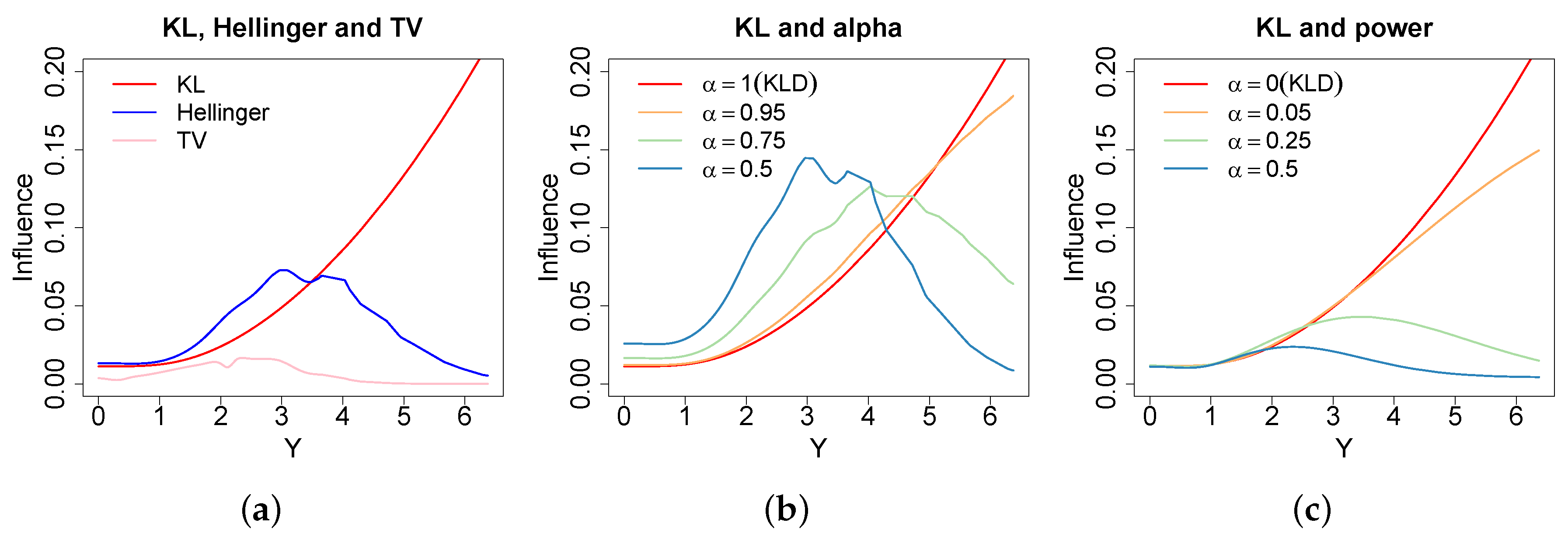
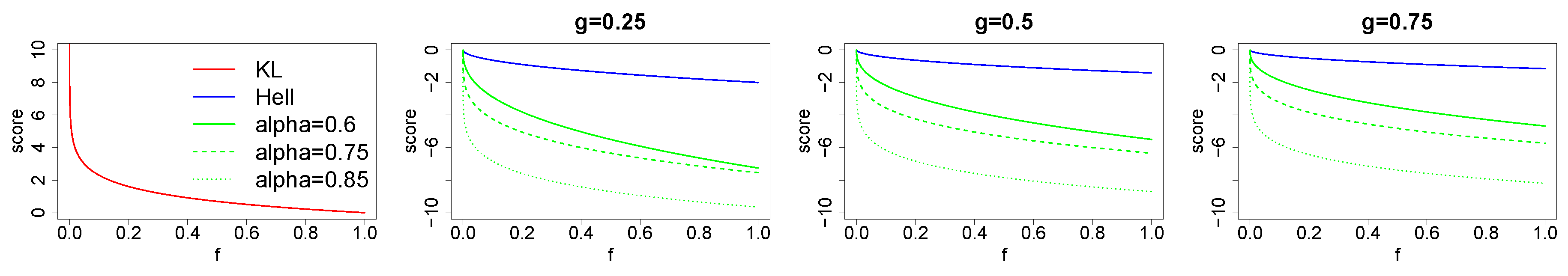
The plots in
Figure 1 demonstrate the influence one observation from a
distribution has on the minimum divergence posterior fitting
, where influence is measured using the method of [
40]. The KL-divergence has a strictly increasing influence function in the observations distance from the mean, so tail observations have large influence over the posterior. As a result, the KL-divergence is suitable if tails are important to the decision problem at hand, but increasing influence characterises a lack of robustness when tails are not important. Alternatively, all of the robust divergence listed above have concave influence functions. The influence of an observation increases as it moves away from the mean, mimicking the behaviour under the KL-divergence, initially, but then decreases as the observations are then declared outliers. The plots for the alpha and power divergence show that changing alpha allows a practitioner to control the level of robustness to tail observations, the values of alpha have been chosen above such that the likelihood is raised to the same power for a given colour across the alpha and power divergence. Influence under the power-divergence is down-weighted according to predicted probabilities under the model. As a result in this high variance example, the down-weighting is quite large. In contrast, the alpha divergence down-weights influence relative to the density estimate allowing observations consistent with this to have much greater influence. Therefore, a density estimate can be used to increase the efficiency of the learning method whilst still maintaining robustness. However, there are clear computational advantages to the power-divergence not requiring a density estimate.
The Hellinger-divergence and the TV-divergence can be selected to provide a fixed level of robustness that is well principled in a decision theoretic manner. Although the TV-divergence is optimal from this point of view, these influence plots show the large reduction in efficiency incurred for using the TV-divergence and this motivates considering the other robust divergence, especially in small sample situations. Once again we stress that we consider the choice of divergence to be a subjective and context specific judgement to be made by the DM similarly to their prior and model.
3.5. Density Estimation
As has been mentioned before, for the TV, Hellinger and
divergence, it is not possible to exactly calculate the loss function associated with any value of
and
x because the data generating density
will not be available. In this case, a density estimate of
is required to produce an empirical loss function. The Bayesian can consider the density estimate as providing additional information to the likelihood from the data (see
Section 2.3.1’s discussion on the likelihood principle), and can thus consider their general Bayesian posterior inferences to be made conditional upon the density estimate as well as the data. The general Bayesian update is a valid update for any loss function, and therefore conditioning on the density estimate as well as the data still provides a valid posterior. However, how well this empirical loss function approximates the exact loss function associated with each divergence ought to be of interest. The exact loss function is of course the loss function the DM would prefer to use having made the subjective judgement to minimise that divergence. If the density estimate is consistent to the data generating process, then provided the sample size is large the density estimate will converge to the data generating density, and the empirical loss function will then correctly approximate the loss function associated with that divergence. It is this fact that ensures the consistency of the posterior estimates of the minimum Hellinger posterior [
16].
Authors [
16] use a fixed width kernel density estimate (FKDE) to estimate the underlying data generating density and in our examples in
Section 4 we adopt this practice using a Radial Basis Function (RBF) kernel for simplicity and convenience. However, we note that [
41] identifies practical drawbacks of FKDEs, including their inability to correctly capture the tails of the data generating process, whilst not over smoothing the centre, as well as the number of data points required to fit these accurately in high dimensions. In addition to this, [
42] observe that the variance of the FKDE when using a density kernel in high dimensions led to asymptotic bias in the estimate that is larger than
. Alternatives include using a kernel with better mean-squared error properties [
43,
44], variable width adaptive KDEs [
45], which [
46] show to be promising in high dimensions, piecewise-constant (alternatively tree based) density estimation [
47,
48] which are also promising in high dimensions, or a fully Bayesian Gaussian process as is recommended in [
49].


