Analysis of Cell Signal Transduction Based on Kullback–Leibler Divergence: Channel Capacity and Conservation of Its Production Rate during Cascade

1
Clinical Research Center for Medical Equipment Development, Kyoto University Hospital, Shogoin-Kawahara-cho 54, Sakyo-ku, Kyoto 606-8057, Japan
2
Department of Drug Discovery Medicine, Pathology Division, Graduate School of Medicine, Kyoto University, Yoshida-Konoe-cho, Sakyo-ku, Kyoto 606-8315, Japan
Entropy 2018, 20(6), 438; https://doi.org/10.3390/e20060438
Submission received: 17 May 2018
/
Revised: 26 May 2018
/
Accepted: 3 June 2018
/
Published: 5 June 2018
(This article belongs to the Section Information Theory, Probability and Statistics)
Abstract
:Kullback–Leibler divergence (KLD) is a type of extended mutual entropy, which is used as a measure of information gain when transferring from a prior distribution to a posterior distribution. In this study, KLD is applied to the thermodynamic analysis of cell signal transduction cascade and serves an alternative to mutual entropy. When KLD is minimized, the divergence is given by the ratio of the prior selection probability of the signaling molecule to the posterior selection probability. Moreover, the information gain during the entire channel is shown to be adequately described by average KLD production rate. Thus, this approach provides a framework for the quantitative analysis of signal transduction. Moreover, the proposed approach can identify an effective cascade for a signaling network.
1. Introduction
Kullback–Leibler divergence (KLD) is a type of generalized entropy or information quantity. It was introduced by Solomon Kullback and Richard A. Leibler, who discussed information source coding theory for information transmission efficiency [1]. At present, KLD finds diverse applications, including the imaging analytical field [2,3], hydrodynamics [4], clinical laboratory tests including electrocardiogram [5,6], network analysis [7,8] for biological applications [9], cellular biology [10], evaluating the bioequivalence of formulations of a drug [11], and experimental design for clinical study [12]. In this study, KLD is applied to analyze the cell information transmission, signal transduction, mediated by the cellular biochemical reaction. In particular, the proposed approach using Bayesian statistics [13,14], which is based on KLD, is expected to provide a novel theoretical framework [7].
Previous studies have discussed cell signal transduction through pathways from a viewpoint of similarity in the thermodynamic process that produces entropy [15]. Luo et al. [16] analyzed the heat production during carbohydrate metabolism and estimated the relationship between energy consumption and biological information from a biological metabolism perspective. Moreover, several research studies have applied variable concepts of entropy. In biologic genome informatics, a type of expanded Shannon entropy, such as the local Shannon-Jayne entropy, is utilized for analyzing the correlation between a set of gene expressions [17,18,19,20,21,22]. Teschendorff et al. [20] introduced a stochastic matrix, whose components are the normalized probabilities of the gene expressions in individual samples; the signal entropy rate was obtained using the matrix. In the network, the maximum entropy rate is determined by the adjacency matrix of the network [20]. For a multi-cell system, the network approach is useful for understanding biological signal transduction behaviors [23,24,25]. Recently, single cell entropy was introduced as the analytical basis of the variable phenotypic or genotypic state of a single cell, which is based on the assembly framework of statistical physics [26]. In another study, using a non-Markovian approach, the mutual entropy between the stimulus and the response in a biological system was considered in a sensory system, wherein the past trajectories are utilized to add useful information to the present state. In a simulation conducted by Becker et al., E. coli was used to reliably predict the concentration changes of environmental chemokines for chemotaxis [27].
Previously, the authors reported analyses of biological signal transduction based on information thermodynamics. In these studies, a theoretical framework was developed on Shannon entropy. However, the objective of the present study is to evaluate signal transduction efficiency of KLD in individual steps on the actual biochemical reaction kinetics [28,29]. KLD is introduced for analysis of signal transduction in reference to fluctuation theorem (FT) [30,31,32,33].
Signal Cascade Model
The signal events can be modeled as a cascade of modification and/or demodification cycle reactions of proteins in a cell that are named signaling molecules. Equation (1) presents a signal cascade model [34,35]. Here, suffixes m and j represent the number of cascades and the step number, respectively. In this model, the signaling molecule at step 1 of cascade m, denoted by Xm1, induces the modification of the Xm2 into Xm2* by binding the signal mediated molecule A such as adenosine triphosphate (ATP). Subsequently, Xm2 activates Xm3 in the same manner. In this way, the signaling molecule at the (j − 1)-th step of cascade m, denoted as Xmj−1, induces the modification of Xmj into Xmj*. As the opposite orientation of signal, demodification of Xmj* into Xmj occurs, at the −(j − 1)-th step of cascade m, and the pre-stimulation steady state is subsequently recovered [34]:
In the above model, the subscript m represents the total number of the cascade.
We introduce a priori (prior) selection probability of signaling molecule for the analysis. Here, qmj, which represents the selection probability of inactive Xmj used in the j-th step in cascade m (forward direction), takes the form of the j-th molecule. On the other hand, qmj*, which represents the selection probability of active Xmj*, is used in the −j-th step for cascade m (backward direction), as follows:
where,
Here, Xm indicates the total concentration of signaling molecules in cascade m:
and the total concentration of active and inactive signaling molecules is given by:
and
The total duration of cascade m, τm0, which indicates the sum of forward and backward cascades comprising a set of signaling molecules, is determined by:
In Equations (2), (5), (6) and (7), the total duration was determined using the probabilities qmj and qmj*:
The suffix 0 represents the prior state. Here, the duration, as forward τmj0 and backward τ−mj0, are defined as shown in Figure 1. The Positive and negative values are assigned to τmj0 and τ−mj0 corresponding to the direction of the step in the m cascade [34,35]. In the above equations, τmj0 represents the duration corresponding to positive code length in which the active molecule Xmj* increases in concentration. On the other hand, τ−mj0 represents the duration corresponding to negative code length in which the active molecule Xmj* decreases in concentration. In this manner, the duration of individual step j-th can be represented as τmj0 − τ−mj0.
2. Results
2.1. A Prior Probability Distribution of Signaling Molecules
Here, the author hypothesizes that the selection of signaling molecules is equal a priori. In our previous studies [34,35], Shannon’s entropy Hm for m-th cascade was demonstrated. Using Equations (3), (5) and (6), entropy Hm0 at a priori (prior) state can be represented as:
To maximize Hm0, using non-determined parameters αm0, and βm0, in reference to the constraints established by Equations (3) and (8), let us introduce a function G.
Then, we have
To maximize G, the right sides of Equations (11)–(13) are equated to zero.
As indicated above, Equations (14) and (15) imply an important result; the coefficient βm0 is independent of the step number j. Therefore, Equations (14) and (15) will be utilized as a prior probability distribution later. Therefore, from Equations (9), (14) and (15) the author has:
2.2. Average Entropy Production Rate in a Signal Cascade
Next, the kinetics were investigated using qm (j|j − 1), which is the transitional probability of the j-th given (j − 1)-th step, and vm (j|j − 1), which is the transitional rate of the j-th step in a forward signaling direction. Given j-th step, qm (j − 1|j) is the transitional probability of the (j − 1)-th step given step j-th step. Similarly, given j-th step, vm (j − 1|j) is the transitional rate of the (j − 1)-th step in a backward signaling direction in a given cascade. The cell system remains at detailed balance around the steady state, the homeostasis, as follows:
Therefore, the author has:
Using kinetic coefficients for (j − 1)-th step and the reverse −(j − 1)-th step, km,j−1 and km,−(j−1) in (1), the right side of (18) is given
When the change of Xm,j−1* is negligible during signal transduction, relative to the fluctuation of Xmj*, we have:
In above, we used Equation (2). Dividing the both sides of above by τmj − τ−mj and taking the limit, the variables qmj and qmj* remain in the right side:
Using Equations (14) and (15), the author has:
In above Equations (22) and (23), |τ−mj0| is sufficiently longer than τmj0, according to experimental studies (Figure 1) [36,37,38,39,40,41,42,43,44,45,46,]. Here, using an arbitrary time parameter t, the average entropy production rate (AEPR), 〈ζmi〉 and 〈ζ−mi〉 are defined during signal transduction for τmj0 − τ−mj0 and |τ−mj0 − τmj0|. respectively for m cascade and reverse cascade −m.
The fluctuation theorem (FT) states that the right sides of Equations (22)–(25) are equal to AEPR
and
Here, βm0 has the dimension of entropy production rate and AEPRs are independent of the step number. Subsequently, AEPRs are redefined using Equations (14), as follows:
Notably, Equations (14), (15) and (28) indicate that AEPR is consistent during signal cascade. Here, the channel capacity is given by AEPR.
2.3. Multinomial Distribution with Population Distribution
KLD was used as a measure of information gain when obtaining a posteriori (posterior) distribution from the prior distribution in Equations (30) and (31) to a posterior distribution. Let probability qmj be the prior distribution. Therefore, the uncertainty reduces:
We define information Dm, as the KLD of signal events in cascade m,
The above equation represents KLD, which indicates the average value of the information obtained from data I with respect to pmj and pmj*. Consequently, KLD is known as information gain. The maximum likelihood estimation is thought to be an estimation method that empirically minimizes KLD.
Posterior probabilities are defined:
and
In addition,
Therefore, when considering the signal transduction occurs under a certain given condition, the probability is transformed from qmj* into pmj* with minimum KLD under the given condition.
To minimize Dm (pmj||qmj) using non-determined parameters αm, and βm in reference to the constraints established by Equations (34) and (36), a function L was introduced to apply Lagrange’s method to undetermined multipliers.
Here, the differences between αm and αm0 and βm0 and βm are indicative of the signaling. Subsequently,
For the minimization of L, the right hand sides of Equations (38)–(40) are equated to zero, as follows:
Therefore, from (41) and (42), the author has
Accordingly, from Equations (7), (43) and (44), KLD is given by:
And the author has:
Accordingly, βm is equal to the average KLD production rate, δ(pm‖qm), during the signal transduction and is consistent during the entire signal cascade. Therefore,
The author defined pm(j|j − 1), which is the transitional probability of the j-th given (j − 1)-th step, and vm(j|j − 1), which is the transitional rate of the j-th step in a forward signaling direction. In addition, given j-th step, pm(j − 1|j) is the transitional probability of the (j − 1)-th step given step j-th step. Similarly, given the j-th step, vm(j − 1|j) is the transitional rate of the (j − 1)-th step in a backward signaling direction in a given cascade.
Likewise from (18)–(20), dividing the both sides of above by τmj − τ−mj and taking the limit, we have:
Further, Equations (47), (50) and (51) give
In above, the author used τmj << τ−mj (Figure 1). Above Equation corresponds to the extended FT considering KLD, and the extended channel capacity can be defined as:
Here, K is an arbitrary constant. If entropy unit is used, K = kB, Boltzmann’s constant. On the other hand, in information science, K is equivalent to log2e.
3. Conclusions
Recently, theoretical analysis of the transduction capacity of biochemical signaling networks has greatly developed [47]. In this study, KLD, the average KLD production rate, and channel capacity based on the average KLD production rate were shown to be critical quantities that can be attributed to the entire signal transduction step. This KLD is a tool to estimate entropy production from stationary trajectories [48].
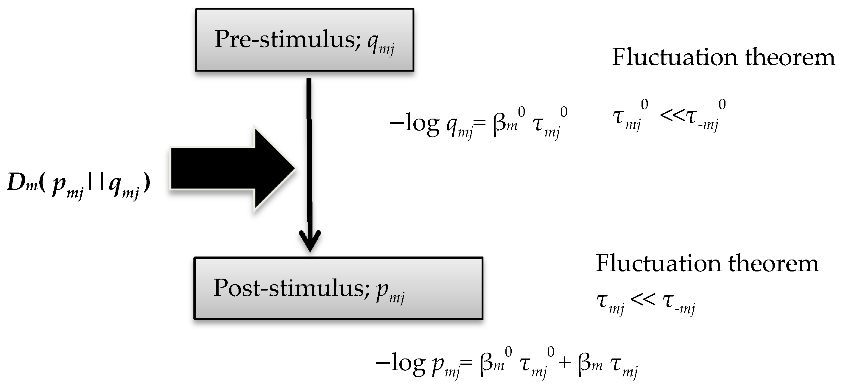
In this work, the author deduced simple but important relational formulae, (47)–(53). For a prior distribution probability qmj, the author derived Equations (14) and (15) in association with FT and source-coding theory [28]. This method was introduced in our previous study of Tsallis entropy [29]. The theoretical framework in the current study is shown in Figure 2.
In this study, uniform distribution was not applied as a prior distribution qmj before stimulus. As reported previously in [34,35], the selection probability of signal molecules, qmj, can be described by simple formulae given by Equations (14) and (15), which illustrate the simple relationship between the logarithm of the probability and time elapsed between tentative modification and demodification. Subsequent to the stimulus, the selection probability of the signal molecules are transformed into a posterior distribution probability pmj. It is likely that the formulation of signal transformation using KLD is more intuitive and easier to understand than using mutual entropy.
The Mitogen-activated Protein Kinase (MAPK) pathway is a multistep signal conversion step, in which the process of modification and demodification in the entire cascade can be understood as a repeated cycle reaction. It has been experimentally demonstrated that the demodification process is significantly longer than the modification process, as shown in τmj << τ−mj (Figure 1), with the former requiring a few hours for completion, while the latter achieves completion in a few minutes. This asymmetry in the time course kinetics points to an important result pertaining the conservation of AEPR and average KLD production rate with reference to FT. In addition, it should be noted that in Equation (53), the channel capacity of the entire signal cascade is represented by KLD. Moreover, the author introduced average KLD production rate in Equation (47), and the production rate was found to be consistent during the whole cascade, which is an expanded form of AEPR conservation during the whole cascade, as reported previously by the author [35].
In the experimental studies [36,37,38,39,40,41,42,43,44,45,46], the ratio of modified active type of signaling molecules was determined by the immunoblot intensity or other corresponding data. Thus, it is possible to compute, in principle, the channel capacity of the entire signal cascade. This can be attributed to the fact that in most cases, extracellular substances, such as ligands, simultaneously promote the activation of multiple cascades. Therefore, the selection of specific ligands for the given cascade is essential and enables the measurement of the rigorous activity of the cascade. In future, such recombinant protein ligand will be required to quantify the signal cascade accurately.
Thus, KLD and average KLD production rate may be regarded as a critical attribution of cell signal cascade. The thermodynamic approach in this manuscript can provide a theoretical framework for the quantitative analysis of signal transduction.
Funding
This research was funded by a Grant-in-Aid from the Ministry of Education, Culture, Sports, Science, and Technology of Japan (Synergy of Fluctuation and Structure: Quest for Universal Laws in Non-Equilibrium Systems, P2013-201 Grant-in-Aid for Scientific Research on Innovative Areas, MEXT, Japan).
Conflicts of Interest
The author declares no conflict of interest.
References
- Kullback, S.; Leibler, R.A. On information and sufficiency. Ann. Math. Stat. 1951, 22, 79–86. [Google Scholar] [CrossRef]
- Liang, S.; Yang, F.; Wen, T.; Yao, Z.; Huang, Q.; Ye, C. Nonlocal total variation based on symmetric kullback-leibler divergence for the ultrasound image despeckling. BMC Med. Imaging 2017, 17, 57. [Google Scholar] [CrossRef] [PubMed]
- Maddux, N.R.; Daniels, A.L.; Randolph, T.W. Microflow imaging analyses reflect mechanisms of aggregate formation: Comparing protein particle data sets using the kullback-leibler divergence. J. Pharm. Sci. 2017, 106, 1239–1248. [Google Scholar] [CrossRef] [PubMed]
- Granero-Belinchon, C.; Roux, S.G.; Garnier, N.B. Kullback-leibler divergence measure of intermittency: Application to turbulence. Phys. Rev. E 2018, 97, 013107. [Google Scholar] [CrossRef] [PubMed]
- Edward Jero, S.; Ramu, P.; Ramakrishnan, S. Discrete wavelet transform and singular value decomposition based ecg steganography for secured patient information transmission. J. Med. Syst. 2014, 38, 132. [Google Scholar] [CrossRef] [PubMed]
- Mager, D.E.; Merritt, M.M.; Kasturi, J.; Witkin, L.R.; Urdiqui-Macdonald, M.; Sollers, J.J., 3rd; Evans, M.K.; Zonderman, A.B.; Abernethy, D.R.; Thayer, J.F. Kullback-leibler clustering of continuous wavelet transform measures of heart rate variability. Biomed. Sci. Instrum. 2004, 40, 337–342. [Google Scholar] [PubMed]
- Arribas, J.I.; Calhoun, V.D.; Adali, T. Automatic bayesian classification of healthy controls, bipolar disorder, and schizophrenia using intrinsic connectivity maps from fmri data. IEEE Trans. Biomed. Eng. 2010, 57, 2850–2860. [Google Scholar] [CrossRef] [PubMed]
- Sun, L.; Ji, S.; Ye, J. Adaptive diffusion kernel learning from biological networks for protein function prediction. BMC Bioinform. 2008, 9, 162. [Google Scholar] [CrossRef] [PubMed]
- Hsiao, C.; Liu, M.; Stanton, R.; McGee, M.; Qian, Y.; Scheuermann, R.H. Mapping cell populations in flow cytometry data for cross-sample comparison using the friedman-rafsky test statistic as a distance measure. Cytometry A 2016, 89, 71–88. [Google Scholar] [CrossRef] [PubMed]
- Wedagedera, J.R.; Burroughs, N.J. T-cell activation: A queuing theory analysis at low agonist density. Biophys. J. 2006, 91, 1604–1618. [Google Scholar] [CrossRef] [PubMed]
- Dragalin, V.; Fedorov, V.; Patterson, S.; Jones, B. Kullback–leibler divergence for evaluating bioequivalence. Stat. Med. 2003, 22, 913–930. [Google Scholar] [CrossRef] [PubMed]
- Cannon, L.; Garcia, C.A.V.; Piovoso, M.J.; Zurakowski, R. Prospective hiv clinical trial comparison by expected kullback-leibler divergence. In Proceedings of the American Control Conference (ACC), Boston, MA, USA, 6–8 July 2016; pp. 1295–1300. [Google Scholar]
- Vogt, M.; Bajorath, J. Bayesian similarity searching in high-dimensional descriptor spaces combined with kullback-leibler descriptor divergence analysis. J. Chem. Inf. Model. 2008, 48, 247–255. [Google Scholar] [CrossRef] [PubMed]
- Wang, C.P.; Ghosh, M. A kullback-leibler divergence for bayesian model diagnostics. Open J. Stat. 2011, 1, 172–184. [Google Scholar] [CrossRef] [PubMed]
- Crofts, A.R. Life, information, entropy, and time: Vehicles for semantic inheritance. Complexity 2007, 13, 14–50. [Google Scholar] [CrossRef] [PubMed] [Green Version]
- Luo, L.-F. Entropy production in a cell and reversal of entropy flow as an anticancer therapy. Front. Phys. China 2009, 4, 122–136. [Google Scholar] [CrossRef] [Green Version]
- Edwards, D.; Wang, L.; Sorensen, P. Network-enabled gene expression analysis. BMC Bioinform. 2012, 13, 167. [Google Scholar] [CrossRef] [PubMed]
- Teschendorff, A.E.; Sollich, P.; Kuehn, R. Signalling entropy: A novel network-theoretical framework for systems analysis and interpretation of functional omic data. Methods 2014, 67, 282–293. [Google Scholar] [CrossRef] [PubMed] [Green Version]
- Sato, M.; Kawana, K.; Adachi, K.; Fujimoto, A.; Yoshida, M.; Nakamura, H.; Nishida, H.; Inoue, T.; Taguchi, A.; Ogishima, J.; et al. Intracellular signaling entropy can be a biomarker for predicting the development of cervical intraepithelial neoplasia. PLoS ONE 2017, 12, e0176353. [Google Scholar] [CrossRef] [PubMed]
- Teschendorff, A.E.; Banerji, C.R.; Severini, S.; Kuehn, R.; Sollich, P. Increased signaling entropy in cancer requires the scale-free property of protein interaction networks. Sci. Rep 2015, 5, 9646. [Google Scholar] [CrossRef] [PubMed]
- Teschendorff, A.E.; Breeze, C.E.; Zheng, S.C.; Beck, S. A comparison of reference-based algorithms for correcting cell-type heterogeneity in epigenome-wide association studies. BMC Bioinform. 2017, 18, 105. [Google Scholar] [CrossRef] [PubMed]
- White, D.R.; Kejzar, N.; Tsallis, C.; Farmer, D.; White, S. Generative model for feedback networks. Phys. Rev. E 2006, 73, 016119. [Google Scholar] [CrossRef] [PubMed] [Green Version]
- Levchenko, A.; Nemenman, I. Cellular noise and information transmission. Curr. Opin. Biotechnol. 2014, 28, 156–164. [Google Scholar] [CrossRef] [PubMed] [Green Version]
- Ellison, D.; Mugler, A.; Brennan, M.D.; Lee, S.H.; Huebner, R.J.; Shamir, E.R.; Woo, L.A.; Kim, J.; Amar, P.; Nemenman, I.; et al. Cell-cell communication enhances the capacity of cell ensembles to sense shallow gradients during morphogenesis. Proc. Natl. Acad. Sci. USA 2016, 113, E679–E688. [Google Scholar] [CrossRef] [PubMed]
- Maire, T.; Youk, H. Molecular-level tuning of cellular autonomy controls the collective behaviors of cell populations. Cell Syst. 2015, 1, 349–360. [Google Scholar] [CrossRef] [PubMed]
- Guo, M.; Bao, E.L.; Wagner, M.; Whitsett, J.A.; Xu, Y. Slice: Determining cell differentiation and lineage based on single cell entropy. Nucleic Acids Res. 2017, 45, e54. [Google Scholar] [CrossRef] [PubMed]
- Becker, N.B.; Mugler, A.; Ten Wolde, P.R. Optimal prediction by cellular signaling networks. Phys. Rev. Lett. 2015, 115, 258103. [Google Scholar] [CrossRef] [PubMed]
- Brillouin, L. Science and Information Theory, 2nd ed.; Dover Publication Inc.: Mineola, NY, USA, 2013; p. 42. [Google Scholar]
- Tsuruyama, T. Channel capacity of coding system on tsallis entropy and q-statistics. Entropy 2017, 19, 682. [Google Scholar] [CrossRef]
- Uda, S.; Kuroda, S. Analysis of cellular signal transduction from an information theoretic approach. Semin. Cell Dev. Biol. 2016, 51, 24–31. [Google Scholar] [CrossRef] [PubMed] [Green Version]
- Sagawa, T.; Kikuchi, Y.; Inoue, Y.; Takahashi, H.; Muraoka, T.; Kinbara, K.; Ishijima, A.; Fukuoka, H. Single-cell E. Coli response to an instantaneously applied chemotactic signal. Biophys. J. 2014, 107, 730–739. [Google Scholar] [CrossRef] [PubMed]
- Ito, S.; Sagawa, T. Maxwell’s demon in biochemical signal transduction with feedback loop. Nat. Commun. 2015, 6, 7498. [Google Scholar] [CrossRef] [PubMed] [Green Version]
- Ito, S.; Sagawa, T. Information thermodynamics on causal networks. Phys. Rev. Lett. 2013, 111, 18063. [Google Scholar] [CrossRef] [PubMed]
- Tsuruyama, T. Information thermodynamics derives the entropy current of cell signal transduction as a model of a binary coding system. Entropy 2018, 20, 145. [Google Scholar] [CrossRef]
- Tsuruyama, T. The conservation of average entropy production rate in a model of signal transduction: Information thermodynamics based on the fluctuation theorem. Entropy 2018, 20, 303. [Google Scholar] [CrossRef]
- Kim, D.S.; Hwang, E.S.; Lee, J.E.; Kim, S.Y.; Kwon, S.B.; Park, K.C. Sphingosine-1-phosphate decreases melanin synthesis via sustained erk activation and subsequent mitf degradation. J. Cell Sci. 2003, 116, 1699–1706. [Google Scholar] [CrossRef] [PubMed]
- Lee, C.S.; Park, M.; Han, J.; Lee, J.H.; Bae, I.H.; Choi, H.; Son, E.D.; Park, Y.H.; Lim, K.M. Liver x receptor activation inhibits melanogenesis through the acceleration of erk-mediated mitf degradation. J. Investig. Dermatol. 2013, 133, 1063–1071. [Google Scholar] [CrossRef] [PubMed]
- Mackeigan, J.P.; Murphy, L.O.; Dimitri, C.A.; Blenis, J. Graded mitogen-activated protein kinase activity precedes switch-like c-fos induction in mammalian cells. Mol. Cell Biol. 2005, 25, 4676–4682. [Google Scholar] [CrossRef] [PubMed]
- Newman, D.R.; Li, C.M.; Simmons, R.; Khosla, J.; Sannes, P.L. Heparin affects signaling pathways stimulated by fibroblast growth factor-1 and-2 in type ii cells. Am. J. Physiol. Lung Cell. Mol. Physiol. 2004, 287, L191–L200. [Google Scholar] [CrossRef] [PubMed]
- Petropavlovskaia, M.; Daoud, J.; Zhu, J.; Moosavi, M.; Ding, J.; Makhlin, J.; Assouline-Thomas, B.; Rosenberg, L. Mechanisms of action of islet neogenesis-associated protein: Comparison of the full-length recombinant protein and a bioactive peptide. Am. J. Physiol. Endocrinol. Metab. 2012, 303, E917–E927. [Google Scholar] [CrossRef] [PubMed]
- Tao, R.; Hoover, H.E.; Honbo, N.; Kalinowski, M.; Alano, C.C.; Karliner, J.S.; Raffai, R. High-density lipoprotein determines adult mouse cardiomyocyte fate after hypoxia-reoxygenation through lipoprotein-associated sphingosine 1-phosphate. Am. J. Physiol. Heart Circ. Physiol. 2010, 298, H1022–E1028. [Google Scholar] [CrossRef] [PubMed]
- Mina, M.; Magi, S.; Jurman, G.; Itoh, M.; Kawaji, H.; Lassmann, T.; Arner, E.; Forrest, A.R.; Carninci, P.; Hayashizaki, Y.; et al. Promoter-level expression clustering identifies time development of transcriptional regulatory cascades initiated by erbb receptors in breast cancer cells. Sci. Rep. 2015, 5, 11999. [Google Scholar] [CrossRef] [PubMed]
- Wang, H.; Ubl, J.J.; Stricker, R.; Reiser, G. Thrombin (par-1)-induced proliferation in astrocytes via mapk involves multiple signaling pathways. Am. J. Physiol. Cell Physiol. 2002, 283, C1351–C1364. [Google Scholar] [CrossRef] [PubMed]
- Wang, Y.Y.; Liu, Y.; Ni, X.Y.; Bai, Z.H.; Chen, Q.Y.; Zhang, Y.; Gao, F.G. Nicotine promotes cell proliferation and induces resistance to cisplatin by alpha7 nicotinic acetylcholine receptor-mediated activation in raw264.7 and el4 cells. Oncol. Rep. 2014, 31, 1480–1488. [Google Scholar] [CrossRef] [PubMed]
- Yeung, K.; Seitz, T.; Li, S.; Janosch, P.; McFerran, B.; Kaiser, C.; Fee, F.; Katsanakis, K.D.; Rose, D.W.; Mischak, H.; et al. Suppression of raf-1 kinase activity and map kinase signalling by rkip. Nature 1999, 401, 173–177. [Google Scholar] [CrossRef] [PubMed]
- Zhang, W.Z.; Yano, N.; Deng, M.Z.; Mao, Q.F.; Shaw, S.K.; Tseng, Y.T. Beta-adrenergic receptor-pi3k signaling crosstalk in mouse heart: Elucidation of immediate downstream signaling cascades. PLoS ONE 2011, 6, e26581. [Google Scholar]
- Cheong, R.; Rhee, A.; Wang, C.J.; Nemenman, I.; Levchenko, A. Information transduction capacity of noisy biochemical signaling networks. Science 2011, 334, 354–358. [Google Scholar] [CrossRef] [PubMed]
- Roldan, E.; Parrondo, J.M. Entropy production and kullback-leibler divergence between stationary trajectories of discrete systems. Phys. Rev. E 2012, 85, 031129. [Google Scholar] [CrossRef] [PubMed]
Figure 1.
A common time course of the j-th step for both prior and posterior cascades, indicating concentration Xmj*. The suffix 0 is omitted. The vertical axis denotes the concentration of signaling active molecule. τmj and τ−mj represent the duration of the j-th step and the reverse −j-th step, respectively. The horizontal line Xmj* = Xmj*st denotes the concentration of Xmj* at the steady state [35]. The “//” symbol on the horizontal axis indicates −τ−mj or |τ−mj| >> τmj.
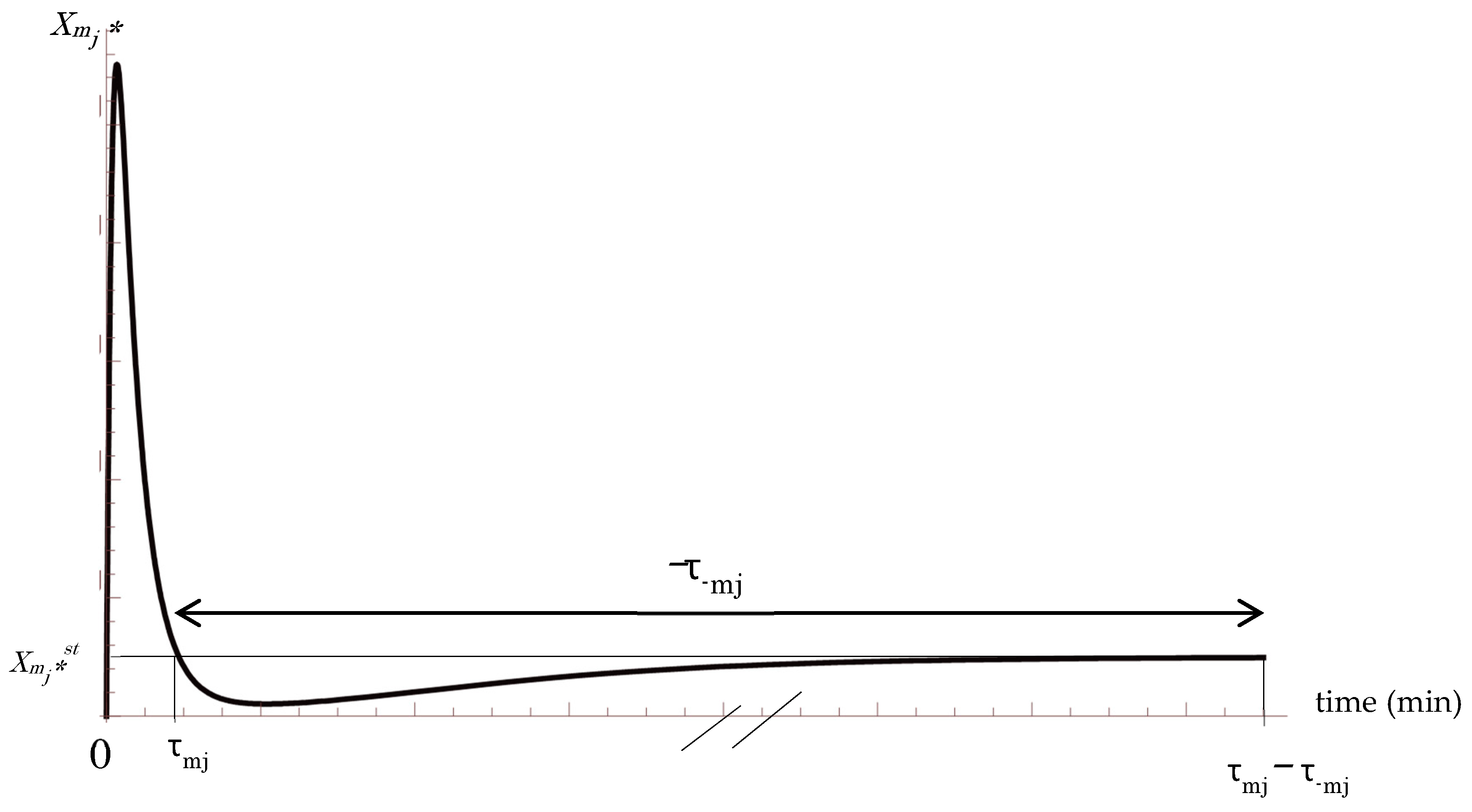
Figure 2.
Theoretical framework of the current study.

© 2018 by the author. Licensee MDPI, Basel, Switzerland. This article is an open access article distributed under the terms and conditions of the Creative Commons Attribution (CC BY) license (http://creativecommons.org/licenses/by/4.0/).
Share and Cite
MDPI and ACS Style
Tsuruyama, T. Analysis of Cell Signal Transduction Based on Kullback–Leibler Divergence: Channel Capacity and Conservation of Its Production Rate during Cascade. Entropy 2018, 20, 438. https://doi.org/10.3390/e20060438
AMA Style
Tsuruyama T. Analysis of Cell Signal Transduction Based on Kullback–Leibler Divergence: Channel Capacity and Conservation of Its Production Rate during Cascade. Entropy. 2018; 20(6):438. https://doi.org/10.3390/e20060438
Chicago/Turabian StyleTsuruyama, Tatsuaki. 2018. "Analysis of Cell Signal Transduction Based on Kullback–Leibler Divergence: Channel Capacity and Conservation of Its Production Rate during Cascade" Entropy 20, no. 6: 438. https://doi.org/10.3390/e20060438
Note that from the first issue of 2016, this journal uses article numbers instead of page numbers. See further details here.