Information Dynamics of a Nonlinear Stochastic Nanopore System


Abstract
1. Introduction
2. Definition and Estimation of Local and Specific Entropy Rates
2.1. Notation
2.2. Differential Entropy and Total Entropy Rate
2.3. Local Entropy Rate
2.4. Specific Entropy Rate
2.5. Specific Information Dynamics with Python
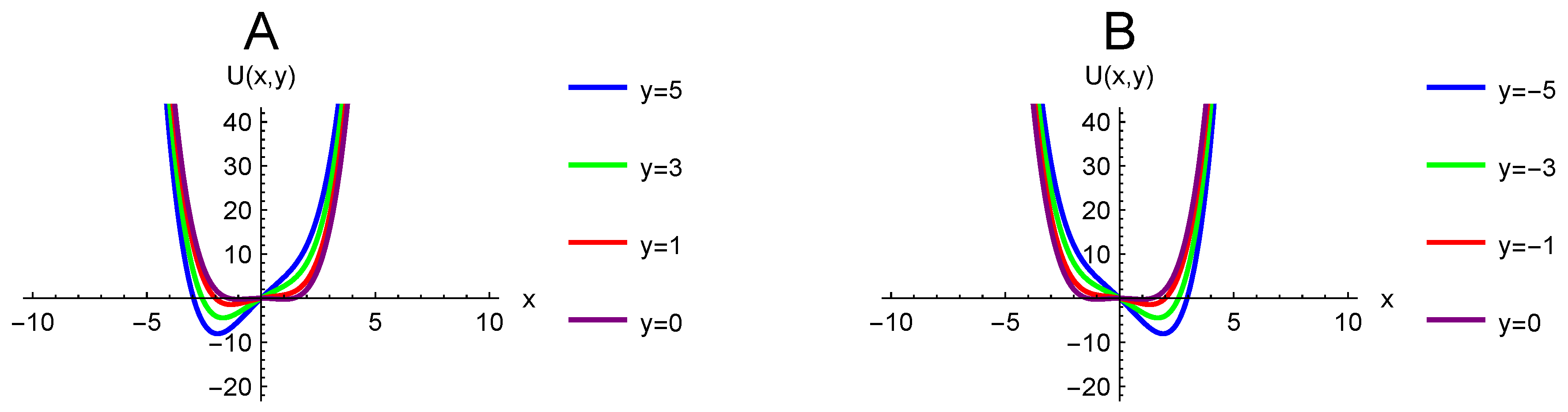
3. Model System
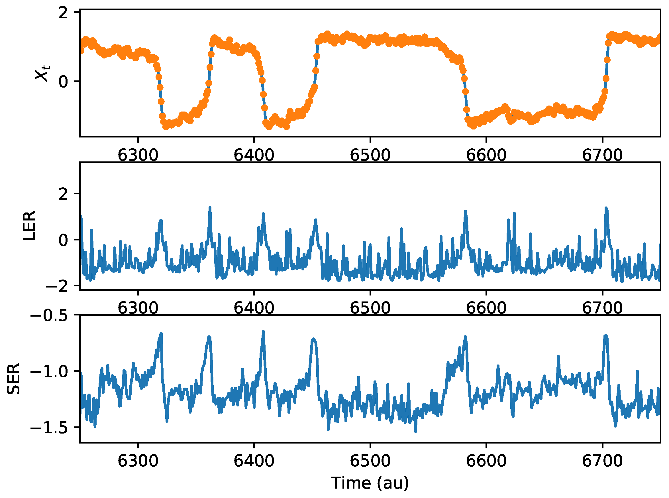
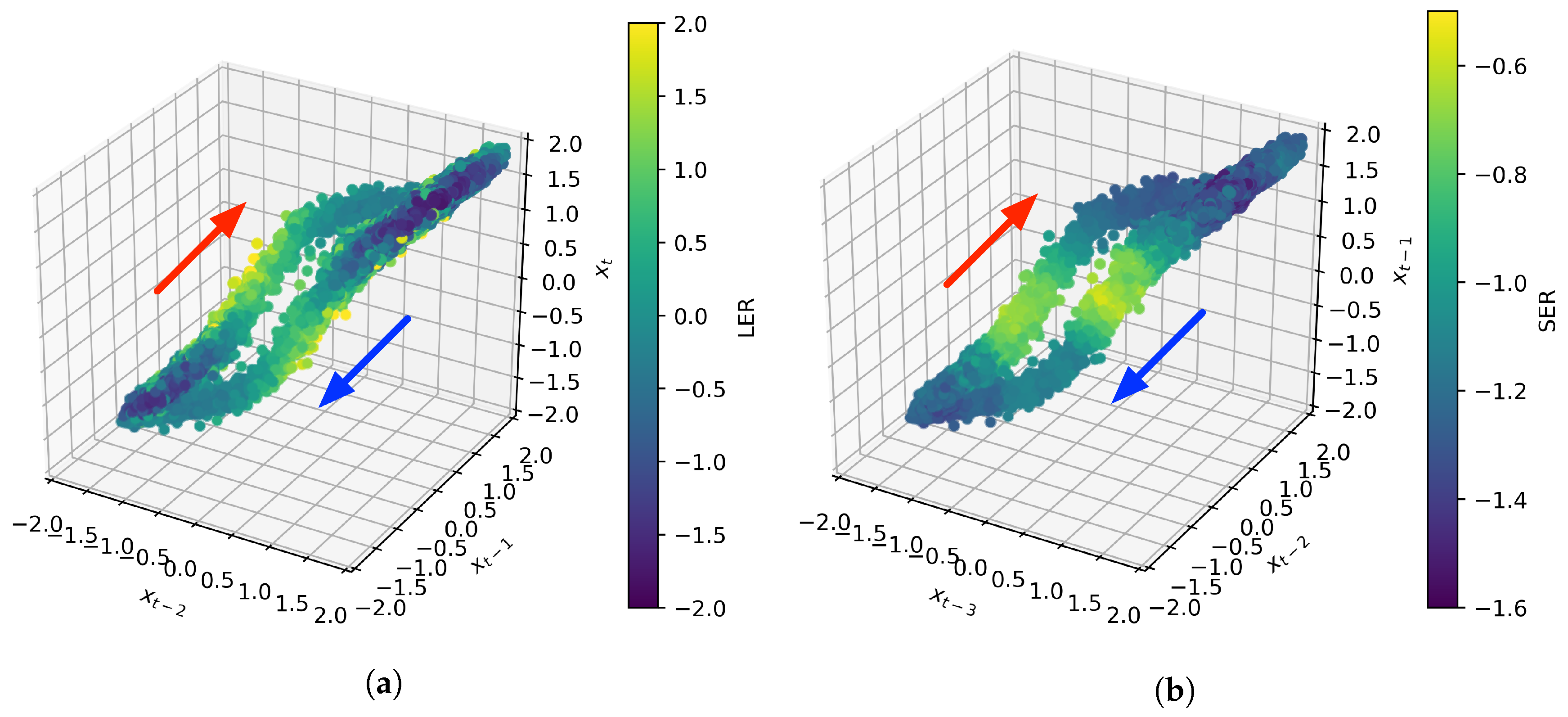
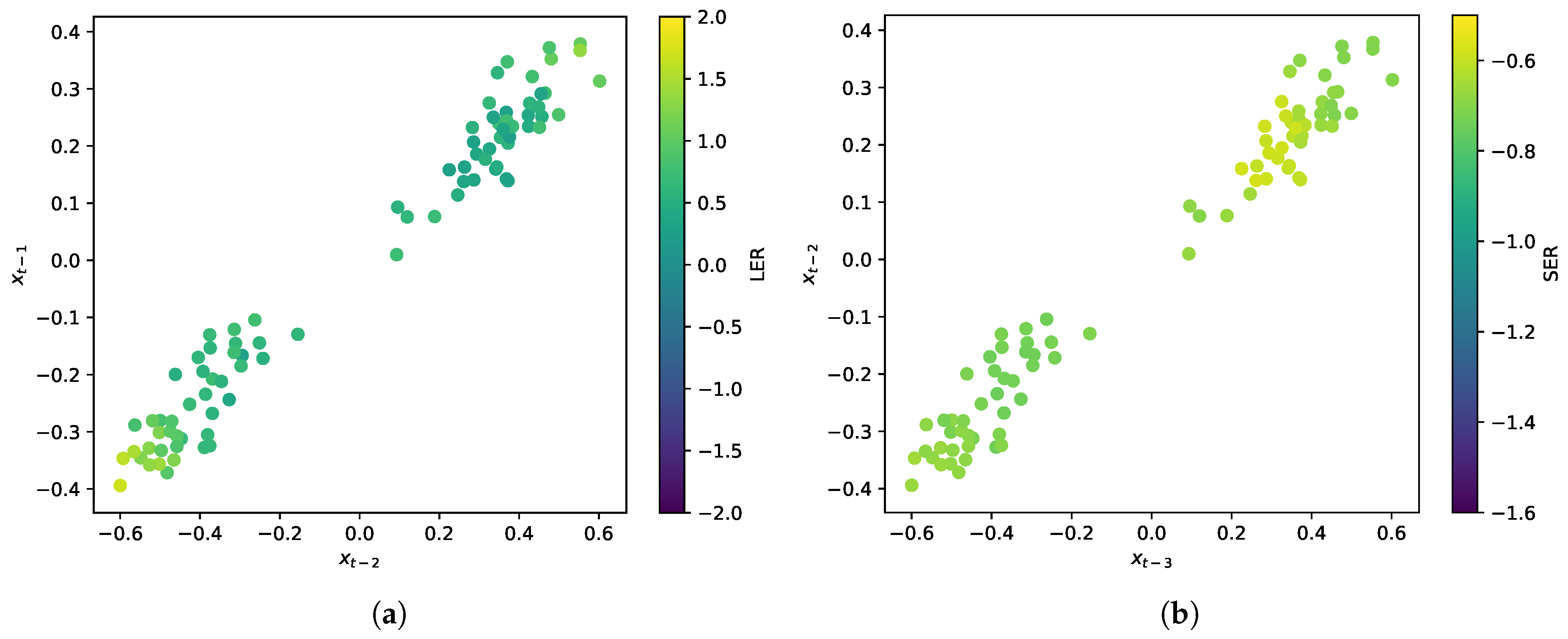
4. Results
5. Discussion
Acknowledgments
Author Contributions
Conflicts of Interest
Abbreviations
| LER | Local entropy rate |
| SER | Specific entropy rate |
| NLPL | Negative log predictive likelihood |
References
- Plett, T.S.; Cai, W.; Le Thai, M.; Vlassiouk, I.V.; Penner, R.M.; Siwy, Z.S. Solid-State Ionic Diodes Demonstrated in Conical Nanopores. J. Phys. Chem. C 2017, 121, 6170–6176. [Google Scholar] [CrossRef]
- Kannam, S.K.; Kim, S.C.; Rogers, P.R.; Gunn, N.; Wagner, J.; Harrer, S.; Downton, M.T. Sensing of protein molecules through nanopores: A molecular dynamics study. Nanotechnology 2014, 25, 155502. [Google Scholar] [CrossRef] [PubMed]
- Kolmogorov, M.; Kennedy, E.; Dong, Z.; Timp, G.; Pevzner, P.A. Single-molecule protein identification by sub-nanopore sensors. PLoS Comput. Biol. 2017, 13, e1005356. [Google Scholar] [CrossRef] [PubMed]
- Howorka, S.; Siwy, Z. Nanopores and Nanochannels: From Gene Sequencing to Genome Mapping. ACS Nano 2016, 10, 9768–9771. [Google Scholar] [CrossRef] [PubMed]
- Innes, L.; Gutierrez, D.; Mann, W.; Buchsbaum, S.F.; Siwy, Z.S. Presence of electrolyte promotes wetting and hydrophobic gating in nanopores with residual surface charges. Analyst 2015, 140, 4804–4812. [Google Scholar] [CrossRef] [PubMed]
- Schiel, M.; Siwy, Z.S. Diffusion and Trapping of Single Particles in Pores with Combined Pressure and Dynamic Voltage. J. Phys. Chem. C 2014, 118, 19214–19223. [Google Scholar] [CrossRef]
- Qiu, Y.; Hinkle, P.; Yang, C.; Bakker, H.E.; Schiel, M.; Wang, H.; Melnikov, D.; Gracheva, M.; Toimil-Molares, M.E.; Imhof, A.; et al. Pores with Longitudinal Irregularities Distinguish Objects by Shape. ACS Nano 2015, 9, 4390–4397. [Google Scholar] [CrossRef] [PubMed]
- Buchsbaum, S.F.; Nguyen, G.; Howorka, S.; Siwy, Z.S. DNA-Modified Polymer Pores Allow pH- and Voltage-Gated Control of Channel Flux. J. Am. Chem. Soc. 2014, 136, 9902–9905. [Google Scholar] [CrossRef] [PubMed]
- Buchsbaum, S.F.; Mitchell, N.; Martin, H.; Wiggin, M.; Marziali, A.; Coveney, P.V.; Siwy, Z.; Howorka, S. Disentangling Steric and Electrostatic Factors in Nanoscale Transport Through Confined Space. Nano Lett. 2013, 13, 3890–3896. [Google Scholar] [CrossRef] [PubMed][Green Version]
- Howorka, S.; Siwy, Z. Nanopores as protein sensors. Nat. Biol. 2012, 30, 506–507. [Google Scholar] [CrossRef] [PubMed]
- Howorka, S.; Siwy, Z. Nanopore analytics: Sensing of single molecules. Chem. Soc. Rev. 2009, 38, 2360–2384. [Google Scholar] [CrossRef] [PubMed]
- Mohammad, M.M.; Movileanu, L. Protein sensing with engineered protein nanopores. Methods Mol. Biol. 2012, 870, 21–37. [Google Scholar] [PubMed]
- Zhang, H.; Tian, Y.; Jiang, L. Fundamental studies and practical applications of bio-inspired smart solid-state nanopores and nanochannels. Nano Today 2016, 11, 61–81. [Google Scholar] [CrossRef]
- Wanunu, M. Nanopores: A journey towards DNA sequencing. Phys. Life Rev. 2012, 9, 125–158. [Google Scholar] [CrossRef] [PubMed]
- Schoch, R.B.; Han, J.; Renaud, P. Transport phenomena in nanofluidics. Rev. Mod. Phys. 2008, 80, 839. [Google Scholar] [CrossRef]
- Tian, Y.; Wen, L.; Hou, X.; Hou, G.; Jiang, L. Bioinspired Ion-Transport Properties of Solid-State Single Nanochannels and Their Applications in Sensing. ChemPhysChem 2012, 13, 2455–2470. [Google Scholar] [CrossRef] [PubMed]
- Pérez-Mitta, G.; Albesa, A.G.; Trautmann, C.; Toimil-Molares, M.E.; Azzaroni, O. Bioinspired integrated nanosystems based on solid-state nanopores: “Iontronic” transduction of biological, chemical and physical stimuli. Chem. Sci. 2017, 8, 890–913. [Google Scholar] [CrossRef] [PubMed]
- Kantz, H.; Schreiber, T. Nonlinear Time Series Analysis; Cambridge University Press: Cambridge, UK, 2004; Volume 7. [Google Scholar]
- Kaplan, D.; Glass, L. Understanding Nonlinear Dynamics; Springer Science & Business Media: New York, NY, USA, 2012. [Google Scholar]
- Lizier, J.T.; Prokopenko, M.; Zomaya, A.Y. Local information transfer as a spatiotemporal filter for complex systems. Phys. Rev. E 2008, 77, 026110. [Google Scholar] [CrossRef] [PubMed]
- Lizier, J.T. Measuring the dynamics of information processing on a local scale in time and space. In Directed Information Measures in Neuroscience; Understanding Complex Systems; Springer: Berlin/Heidelberg, Germany, 2014; pp. 161–193. [Google Scholar]
- Lizier, J.T. JIDT: An information-theoretic toolkit for studying the dynamics of complex systems. arXiv, 2014; arXiv:1408.3270. [Google Scholar]
- Wibral, M.; Lizier, J.T.; Vögler, S.; Priesemann, V.; Galuske, R. Local active information storage as a tool to understand distributed neural information processing. Front. Neuroinf. 2014, 8, 1. [Google Scholar] [CrossRef] [PubMed]
- Darmon, D. Specific differential entropy rate estimation for continuous-valued time series. Entropy 2016, 18, 190. [Google Scholar] [CrossRef]
- Hyland, B.; Siwy, Z.S.; Martens, C.C. Nanopore Current Oscillations: Nonlinear Dynamics on the Nanoscale. J. Phys. Chem. Lett. 2015, 6, 1800–1806. [Google Scholar] [CrossRef] [PubMed]
- Powell, M.R.; Sullivan, M.; Vlassiouk, I.; Constantin, D.; Sudre, O.; Martens, C.C.; Eisenberg, R.S.; Siwy, Z.S. Nanoprecipitation-assisted ion current oscillations. Nat. Nanotechnol. 2008, 3, 51. [Google Scholar] [CrossRef] [PubMed]
- Turker Acar, E.; Hinkle, P.; Siwy, Z.S. Concentration Polarization Induced Precipitation and Ionic Current Oscillations with Tunable Frequency. J. Phys. Chem. C 2018, 122, 3648–3654. [Google Scholar] [CrossRef]
- Caires, S.; Ferreira, J.A. On the non-parametric prediction of conditionally stationary sequences. Stat. Inference Stoch. Process. 2005, 8, 151–184. [Google Scholar] [CrossRef]
- Cover, T.M.; Thomas, J.A. Elements of Information Theory; John Wiley & Sons: New York, NY, USA, 2012. [Google Scholar]
- Simonoff, J.S. Smoothing Methods in Statistics; Springer Science & Business Media: New York, NY, USA, 2012; pp. 124–125. [Google Scholar]
- Darmon, D. Information-theoretic model selection for optimal prediction of stochastic dynamical systems from data. Phys. Rev. E 2018, 97, 032206. [Google Scholar] [CrossRef]
- Lincheng, Z.; Zhijun, L. Strong consistency of the kernel estimators of conditional density function. Acta Math. Sin. 1985, 1, 314–318. [Google Scholar] [CrossRef]
- Izbicki, R.; Lee, A.B. Nonparametric conditional density estimation in a high-dimensional regression setting. J. Comput. Graph. Stat. 2016, 25, 1297–1316. [Google Scholar] [CrossRef]
- Nelder, J.A.; Mead, R. A simplex method for function minimization. Comput. J. 1965, 7, 308–313. [Google Scholar] [CrossRef]
- Biau, G.; Devroye, L. Lectures on the Nearest Neighbor Method; Springer: Berlin, Germany, 2015. [Google Scholar]
- Darmon, D.; Rapp, P.E. Specific transfer entropy and other state-dependent transfer entropies for continuous-state input-output systems. Phys. Rev. E 2017, 96, 022121. [Google Scholar] [CrossRef] [PubMed]
- Loftsgaarden, D.O.; Quesenberry, C.P. A Nonparametric Estimate of a Multivariate Density Function. Ann. Math. Stat. 1965, 36, 1049–1051. [Google Scholar] [CrossRef]
- Wagner, T.J. Strong Consistency of a Nonparametric Estimate of a Density Function. IEEE Trans. Syst. Man Cybern. 1973, SMC-3, 289–290. [Google Scholar]
- Moore, D.S.; Yackel, J.W. Consistency Properties of Nearest Neighbor Density Function Estimators. Ann. Stat. 1977, 5, 143–154. [Google Scholar] [CrossRef]
- Darmon, D. Specific Information Dynamics with Python (sidpy), Version 0.1. 2018. Available online: https://github.com/ddarmon/sidpy (accessed on 28 February 2018).
- Wen, C.; Zeng, S.; Zhang, Z.; Hjort, K.; Scheicher, R.; Zhang, S.L. On nanopore DNA sequencing by signal and noise analysis of ionic current. Nanotechnology 2016, 27, 215502. [Google Scholar] [CrossRef] [PubMed]
- Rößler, A. Runge–Kutta methods for the strong approximation of solutions of stochastic differential equations. SIAM J. Numer. Anal. 2010, 48, 922–952. [Google Scholar] [CrossRef]


© 2018 by the authors. Licensee MDPI, Basel, Switzerland. This article is an open access article distributed under the terms and conditions of the Creative Commons Attribution (CC BY) license (http://creativecommons.org/licenses/by/4.0/).
Share and Cite
Gilpin, C.; Darmon, D.; Siwy, Z.; Martens, C. Information Dynamics of a Nonlinear Stochastic Nanopore System. Entropy 2018, 20, 221. https://doi.org/10.3390/e20040221
Gilpin C, Darmon D, Siwy Z, Martens C. Information Dynamics of a Nonlinear Stochastic Nanopore System. Entropy. 2018; 20(4):221. https://doi.org/10.3390/e20040221
Chicago/Turabian StyleGilpin, Claire, David Darmon, Zuzanna Siwy, and Craig Martens. 2018. "Information Dynamics of a Nonlinear Stochastic Nanopore System" Entropy 20, no. 4: 221. https://doi.org/10.3390/e20040221
APA StyleGilpin, C., Darmon, D., Siwy, Z., & Martens, C. (2018). Information Dynamics of a Nonlinear Stochastic Nanopore System. Entropy, 20(4), 221. https://doi.org/10.3390/e20040221