1. Introduction
The association between random variables is a subject of interest in many scientific fields. The most complete method of characterizing the association between random variables is to determine the joint distribution of these random variables. Multivariate density functions, for absolutely continuous variables, and multivariate probability mass functions, for discrete variables, have become the focus of researchers interested in evaluating such associations (see, for example, [
1,
2,
3,
4]).
The motivation for the present paper was a study performed as part of the Obsessive-Compulsive Spectrum Disorder Program of the Institute of Psychiatry, University of São Paulo Medical School. A group of 1001 consecutive adult outpatients diagnosed with primary obsessive-compulsive disorder (OCD) according to the DSM-IV criteria [
5] were recruited, and some of these patients were submitted to psychiatric treatment. Their OCD severity was evaluated using the Yale-Brown Scale (YBOCS; [
6,
7]) at the beginning of the project. At the time when the data records were accessed, only 213 patients participated in the re-evaluation using the same scale. The YBOCS is composed of two sub-scales, obsession (O) and compulsion (C), and each sub-scale assumes values in the set of integers
. To measure the OCD severity of the patients, we considered the maximum value between the O and C sub-scale measures, max{O;C}; this method of scoring is known as the M-YBOCS scale (see the discussions in [
8,
9]).
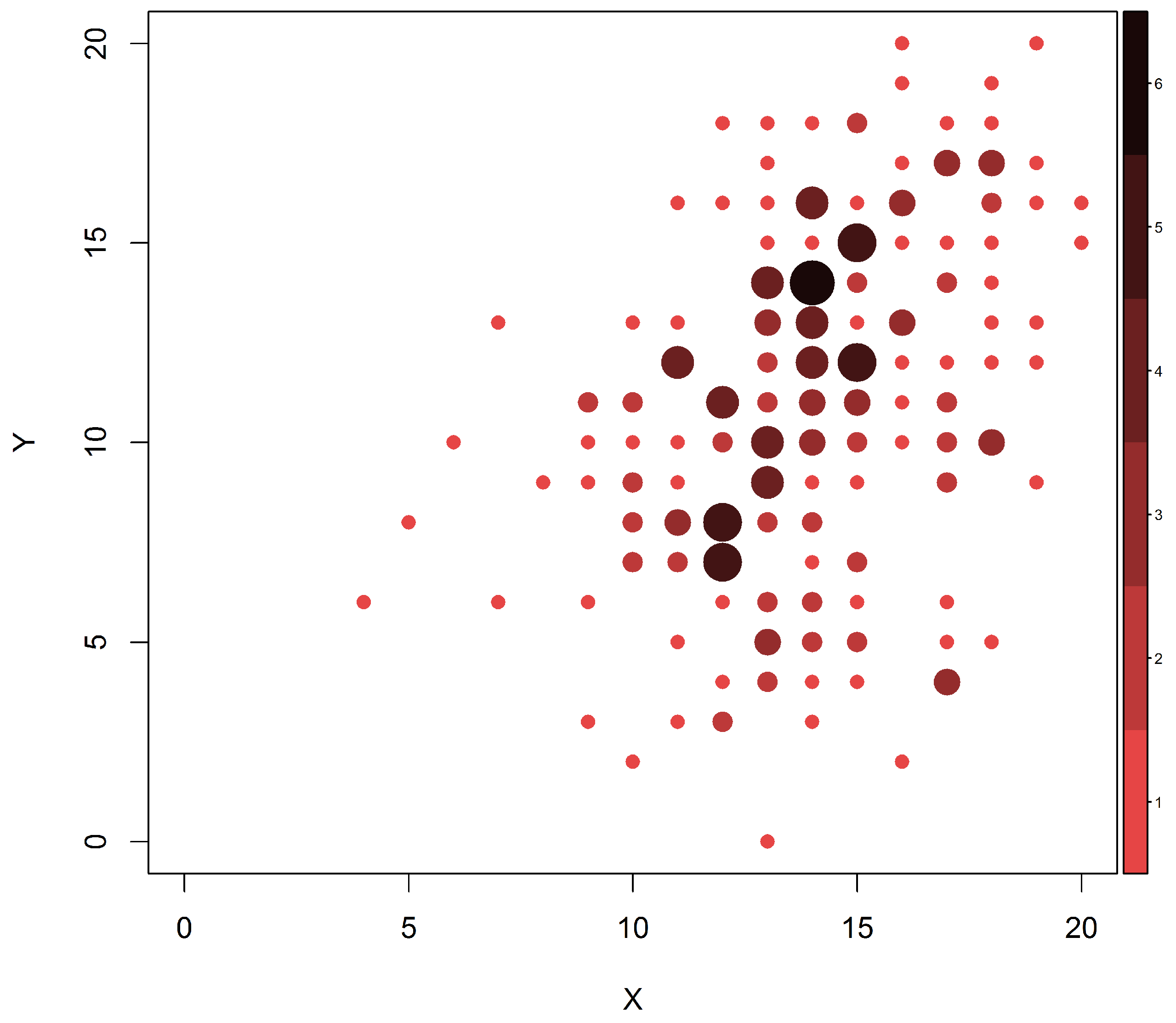
Figure 1 presents the initial (
X) and final (
Y) M-YBOCS scores for all 213 patients for whom both initial and final scores were obtained. In this graphic, darker colors and larger dots represent higher cell frequencies. Our first objective is to estimate the marginal distributions of the initial and final scores. For this purpose, all available information should be used: all 1001 patients included in the first evaluation and all 213 remaining patients at the end of the study. If we use only the complete pairs of observation, omitting missing marginal values, we obtain only 213 pairs of measurements to be used in the estimation of the joint distribution of interest, the support of which possibly contains
points, nearly double the sample size. As a consequence, standard methods of estimation (like maximum likelihood) would unavoidably yield estimates equal to zero for most cell probabilities. It is then reasonable to consider the whole dataset (including the available incomplete pairs) in order to improve such estimates.
The objective of the present paper is to introduce a method of estimating multivariate discrete probability mass functions in the presence of (marginal) missing data. For this purpose, we developed an estimation method that uses both empirical distribution functions and Bernstein polynomials. The procedure consists of estimating a smooth joint distribution function, followed by applying a method that transforms this function into a discrete function, i.e., the estimated joint probability mass function. The results of this new method are compared with those of alternative methods, both graphically and by evaluating standard distances.
Section 2 describes the existing methods found in the literature that will be considered for comparison.
Section 3 describes our estimator for the joint probability functions.
Section 4 presents a discussion of the new method and comparisons of this method to the alternative methods using both simulated samples and the real OCD example. Finally, in
Section 5, we present our final comments and considerations for future work.
2. Existing Solutions
First, we introduce the mathematical framework for our problem. Let F be the unknown distribution function of a random vector that takes values in a subset of . A sample of size n of is represented by , where and . In other words, the ’s are conditionally independent and identically distributed random variables, given any distribution function F. Observations of are denoted by .
Assuming that the distribution
F is drawn from a known family of distributions, we represent the statistical model by
, where
is the sample space,
is a sigma-algebra of its subsets and
is a family of distributions indexed by the parameter
that belongs to the parameter space
. The estimation of
F is then reduced to that of the parameter
, and the dependence structure is limited to that supported by the underlying statistical model. For many years, the multivariate normal distribution has been used for most multivariate analyses (see, for example, [
10,
11]). Recently, for many random phenomena whose distributions are skewed and possess heavier tails than those of the normal distribution, alternative distributions, such as multivariate skew-elliptical distributions, have been adopted [
12,
13].
In recent approaches, copulas have become a popular tool for modeling multivariate dependence structures and for obtaining new multivariate distributions with given marginals. In short, a copula is a multivariate distribution whose marginals are uniform over the entire range
. There are many parametric families of copulas, allowing for the modeling of many different dependence structures [
1,
2,
3,
4]. Let
F be a
p-dimensional distribution function with the margins
. Sklar [
14] first showed that there exists a
p-dimensional copula
C such that:
for all
in the domain of
F. If the variables
are absolutely continuous, then the copula
C is unique; otherwise,
C is uniquely determined on
, where
is the image of the function
,
[
14]. Thus, the copula can be used to separately model the margins and the dependence structure. The non-unique representation of a copula for discrete distributions is a theoretical issue that must be considered in the context of an analytical proof, but this does not limit its empirical applications [
15]. However, the above theorem [
14] does not tell us how to find the copula
C. This problem is widely discussed in the literature, and several solutions to this problem have been proposed (see, for example, [
16]). The most widely-used approach is to adjust several families of (parametric) copulas and choose one of them using certain selection criteria or a goodness-of-fit test [
17,
18,
19,
20,
21].
Nonparametric techniques may also be applied to estimate a multivariate distribution. A popular solution using this approach is the application of the empirical distribution function
, which is defined, for
, as:
where
is the indicator of the set
A. This approach is equivalent to using the relative frequencies to estimate the joint probability mass function. The relative frequencies coincide with the maximum-likelihood estimate under the assumption that the data are drawn from a multinomial distribution. One shortcoming of such approaches is that the probability of any non-observed cells will be estimated to be zero.
Another possible approach is to use some function to smooth the empirical distribution. We can consider the Bernstein polynomials [
22,
23] for this purpose because of their simplicity and good mathematical properties [
24,
25]. Let
be a continuous function. The
mth-degree (multivariate) Bernstein polynomial for the function
h, namely,
, is defined as:
The multivariate Bernstein polynomials for the function
h converge uniformly to the function
h as
[
26,
27], and its derivatives are simple to obtain. The function
h must be defined in
, and therefore, for practical purposes, data that do not take values in
must first be transformed [
24]. To apply this method to the OCD data, for example, we consider the transformation
. Moreover, the polynomial degree adopted here is
, as suggested by [
24]. Bernstein polynomials have been used to approximate a copula
C by simply replacing the function
h with the copula. The resulting Bernstein polynomial,
, which is also a copula that strongly converges to
C, is called a Bernstein copula [
28,
29,
30,
31,
32]. When the true copula is unknown, the empirical copula can be used instead, and the resulting function is called the empirical Bernstein copula [
16,
33,
34,
35,
36,
37]. The empirical copula is defined as:
Note that even when
,
, is unknown, we can use the empirical marginal distribution
as a consistent estimator of
, according to the Glivenko–Cantelli theorem (e.g., [
38]). Other estimators for marginal distributions could be considered instead, as in the procedure proposed in the next section.
We have so far obtained a continuous function as an estimate while our objective is clearly to estimate a (discrete) probability mass function. Hence, this function must be discretized to obtain an adequate estimate. This can be achieved as follows: suppose, with no loss of generality, that
is a random vector such that all its components
,
, assume values in the set
with probability one. In addition, there always exists a continuous random vector
with distribution function
F such that
,
, and
,
i. It follows that:
Let
F (or an estimate
) be the continuous joint distribution function of the random vector
, and let
be a
p-dimensional rectangle with all its vertices in
. The
F-volume of
B [
4] is then given by:
where the sum is taken over all vertices
of
B, and
is given by:
In particular, suppose
, and take
, with
,
, then the probability of the event
can be calculated (estimated) as:
Because weak convergence occurs at the points of continuity of the limiting distribution function F and because our goal is to estimate a discrete probability mass function, we consider sets of the form , with , so that the vertices of the p-dimensional rectangle B are always points of continuity of the distribution function of the discrete random vector . Thus, such discretization yields satisfactory estimates for the probability mass function of .
3. Proposed Solutions
Our proposed method for estimating the joint distribution of a discrete random vector consists of using Bernstein polynomials to estimate both the marginals and the copula. The advantage of this method is that it allows all observations to be used, even in the case of missing values in some variable. Furthermore, this method is a nonparametric approach, and there are few restrictions on the dependence structure.
First, for each random variable
, we estimate the marginal distributions using the empirical marginal distribution with
observations,
,
; then, the Bernstein polynomial of degree
is used to smooth this function:
As this estimator converges to the marginal distribution [
24], we estimate the copula using an alternative version of the empirical copula based on the
n complete observations and the estimates
,
,
and smooth this function to obtain the corresponding empirical Bernstein copula,
Note that the construction of the copula
using Bernstein polynomials rather than empirical (marginal) distribution functions yields, at least in the examples to be presented in
Section 4, non-zero estimates for non-observed cells. This feature justifies the choice of this alternative version of the empirical copula.
The estimate of the joint distribution function is a discretization (Equation (
3)) of the following function:
The algorithm used to obtain the proposed solution is quite simple and is summarized below:
for all observations of each variable , estimate the marginal empirical distribution function ;
smooth each function using a Bernstein polynomial of degree ;
for all complete observations of the random vector , estimate the empirical copula ;
estimate the Bernstein copula by smoothing the empirical copula using the mth-degree multivariate Bernstein polynomial ;
obtain a continuous estimate of the multivariate distribution function
given by Equation (
4);
discretize
using Equation (
3) to obtain an estimate of the discrete multivariate probability mass function.
4. Applications
To evaluate the robustness of the method, we simulated datasets from two bivariate discrete distributions generated using copulas (Examples 4.1 and 4.2). For each simulated example, we present the estimated probabilities for three cases:
600 pairs of observations with no censored data;
censored data in only one marginal, with 1000 observations in one marginal and 200 in another; and
censored data in both variables, with 600 observations for each variable, 300 of which form complete pairs.
After these examples, we present and compare estimates to the observed data from the OCD study (Example 4.3).
For the examples described above, we present the estimates for the probability mass functions considering the proposed method and compare its performance with some existing solutions, similar to those briefly discussed in
Section 2 and which are more detailed below:
the empirical distribution presented in Equation (
1), that is obtained using only the complete pairs and the resulting probability function, coincides with the relative frequencies of the points observed in the sample;
the multivariate skew t approximation that is obtained through a discretization of a parametric multivariate continuous distribution, estimated by the maximum likelihood method using only the complete pairs;
the discretization of the normal copula with the normal marginal approximation to the distribution function that is obtained by using all observations for marginal distribution estimation and using only the complete pairs for copula estimation. This method is quite similar to that described in (b) considering the normal multivariate distribution rather than the skew t distribution, but here, it is possible to estimate the marginal distributions using all available data, not just the complete pairs;
the discretization of the empirical Bernstein polynomial approximation presented in Equation (
2), replacing the function
h by the empirical distribution
obtained in (a) and using only the complete pairs; and
our proposed solution described in the previous section, which is obtained by using the Bernstein polynomial to approximate the margins using all observations and the approximated copula using the complete pairs.
For all examples, we graphically illustrate the estimates of the probability mass distributions and evaluate several distances between the estimated and theoretical distributions. For this purpose, some notation must be introduced. Let be the theoretical probabilities, and let be the estimated probabilities. We consider the following distances for comparison of the estimates:
Total variation distance:
Kullback–Leibler symmetrized divergence:
Aitchison [
39,
40] and Pawlowsky [
41] have presented many arguments for using Aitchison’s distance for compositional vectors, that is when the sum of the vector’s components is constant (in our case, the sum of the probabilities is equal to one). Moreover, the orderings implied by these distances agree in most cases.
At the end of this section, we present the estimates for the distribution of the real data described in the Introduction. In this case, we do not know the theoretical distribution; we present only the estimates and the distances calculated from the empirical distribution.
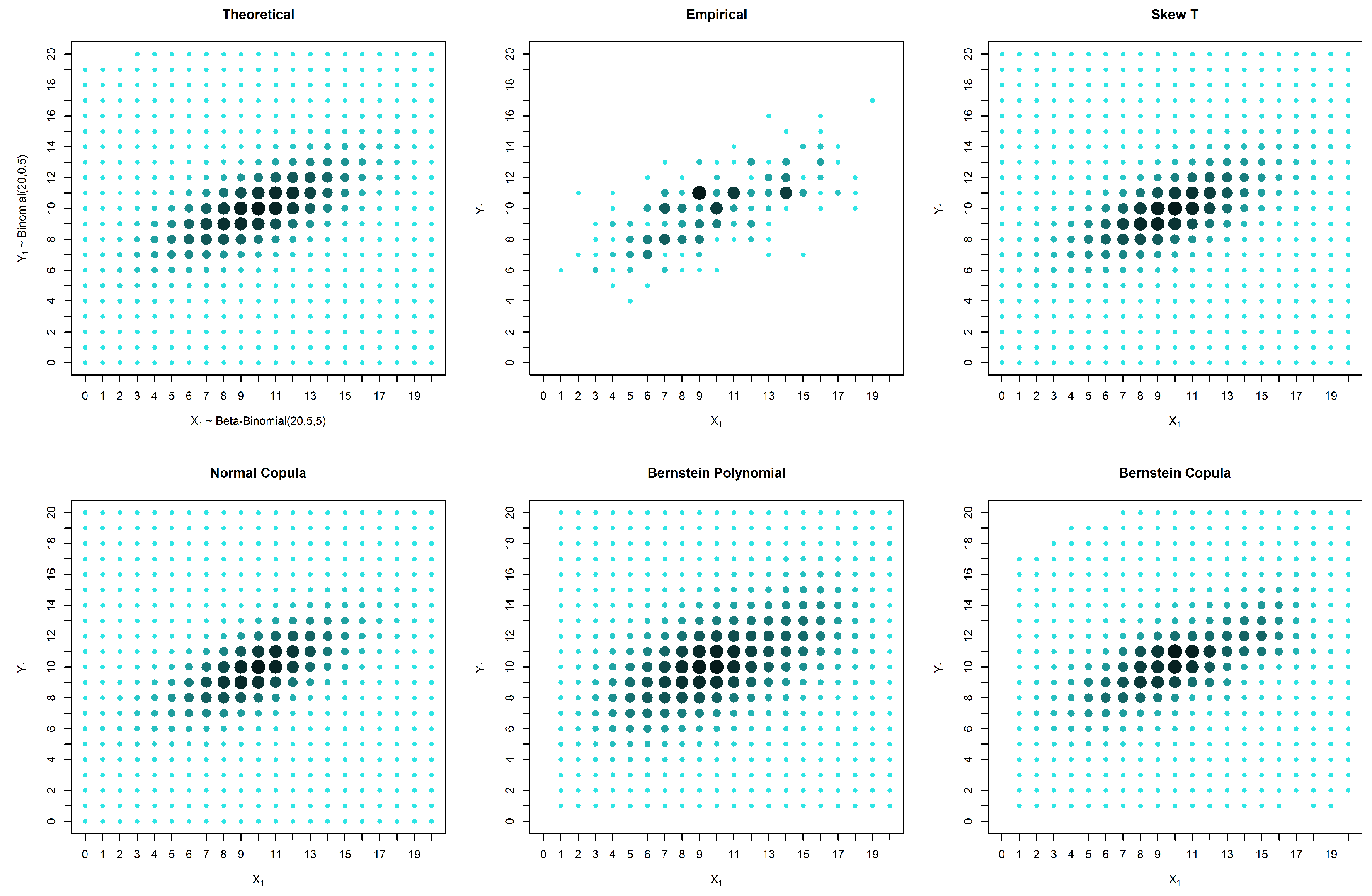
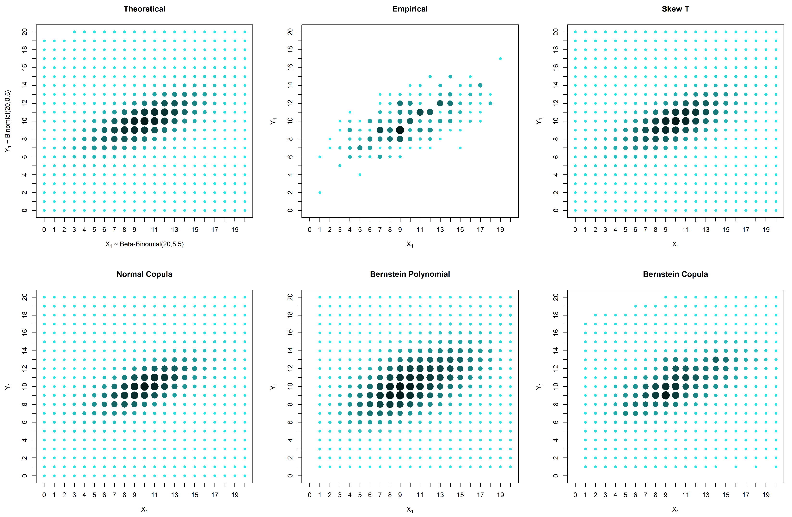
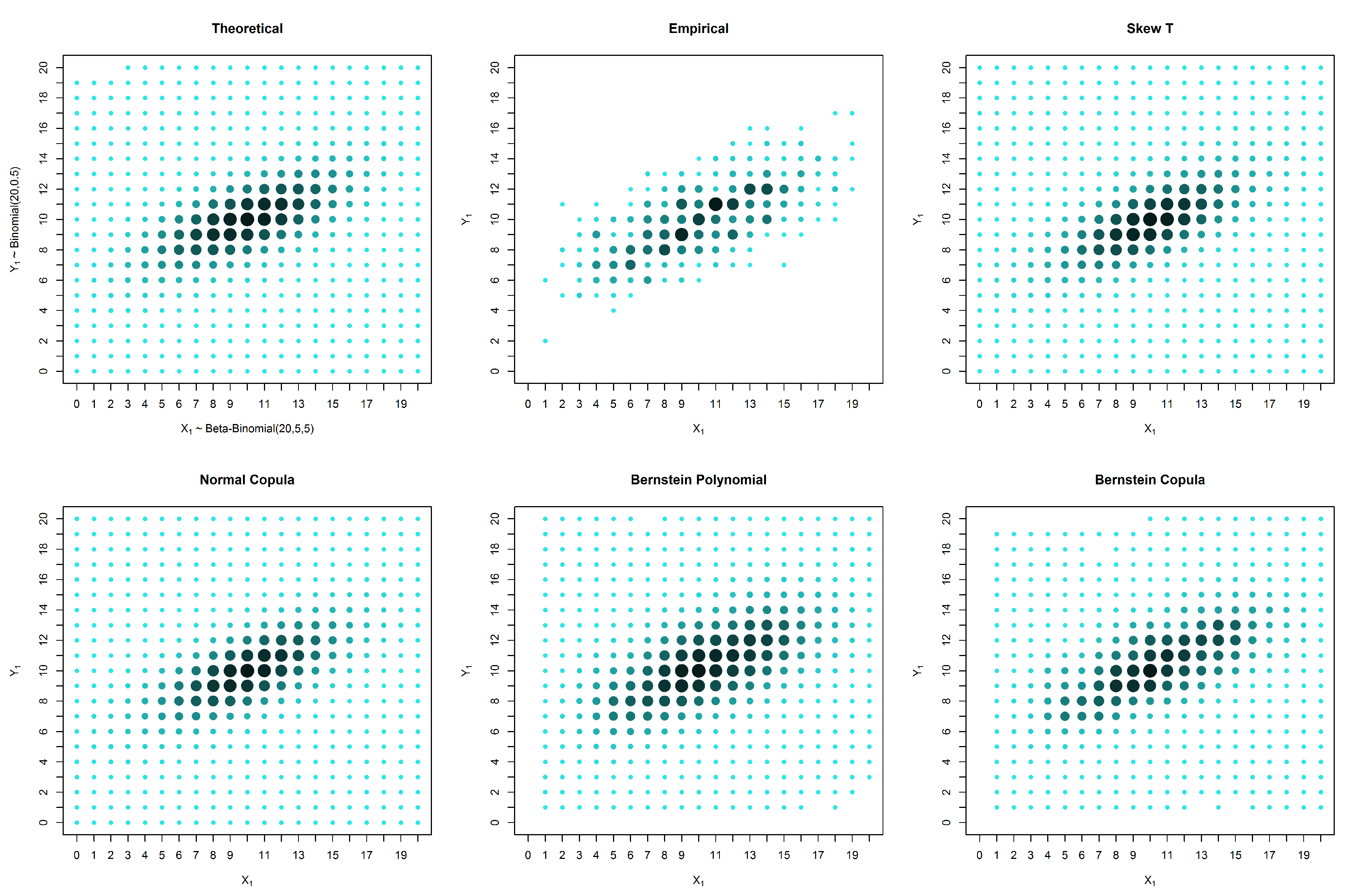
4.1. Simulated Elliptically-Shaped Distribution
In this section, we simulate data from an elliptically-shaped distribution with marginals and and a normal copula with parameter .
We can see from
Figure 2,
Figure 3 and
Figure 4 and from
Table 1,
Table 2 and
Table 3 that in these examples, the solutions based on elliptical distributions, namely the skew t and normal distributions, yield better estimates. This superior estimation occurs because the theoretical probability mass function is elliptical in shape. However, in practical situations, we have no knowledge of the real shape of the distribution. In such a case, the empirical distribution may be a good basis for evaluating the estimates, despite the existence of many unobserved points that are estimated as zero. When the estimates are compared with the empirical distribution, our proposed solution appears to produce good results, particularly in the presence of censored data.
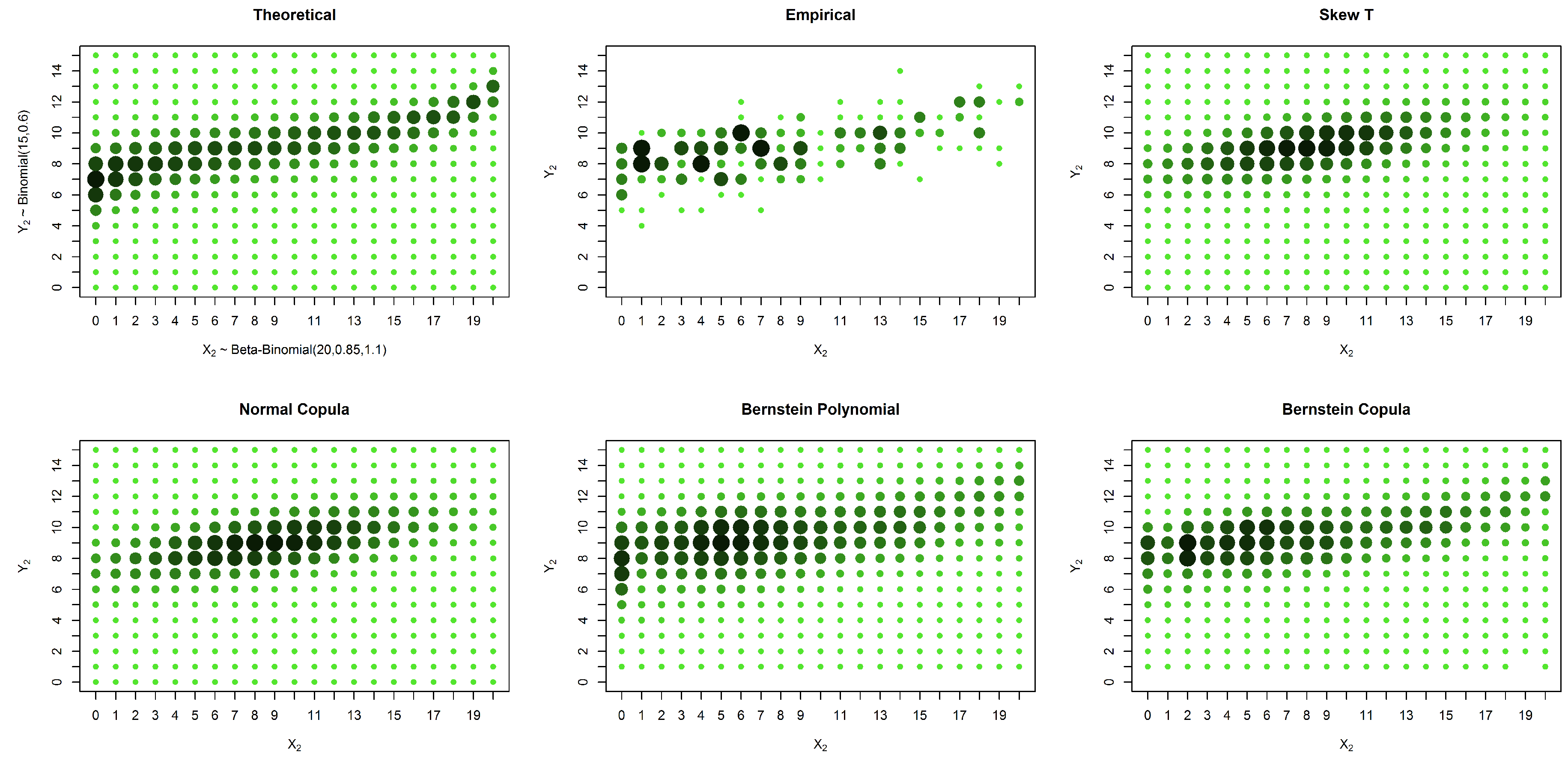
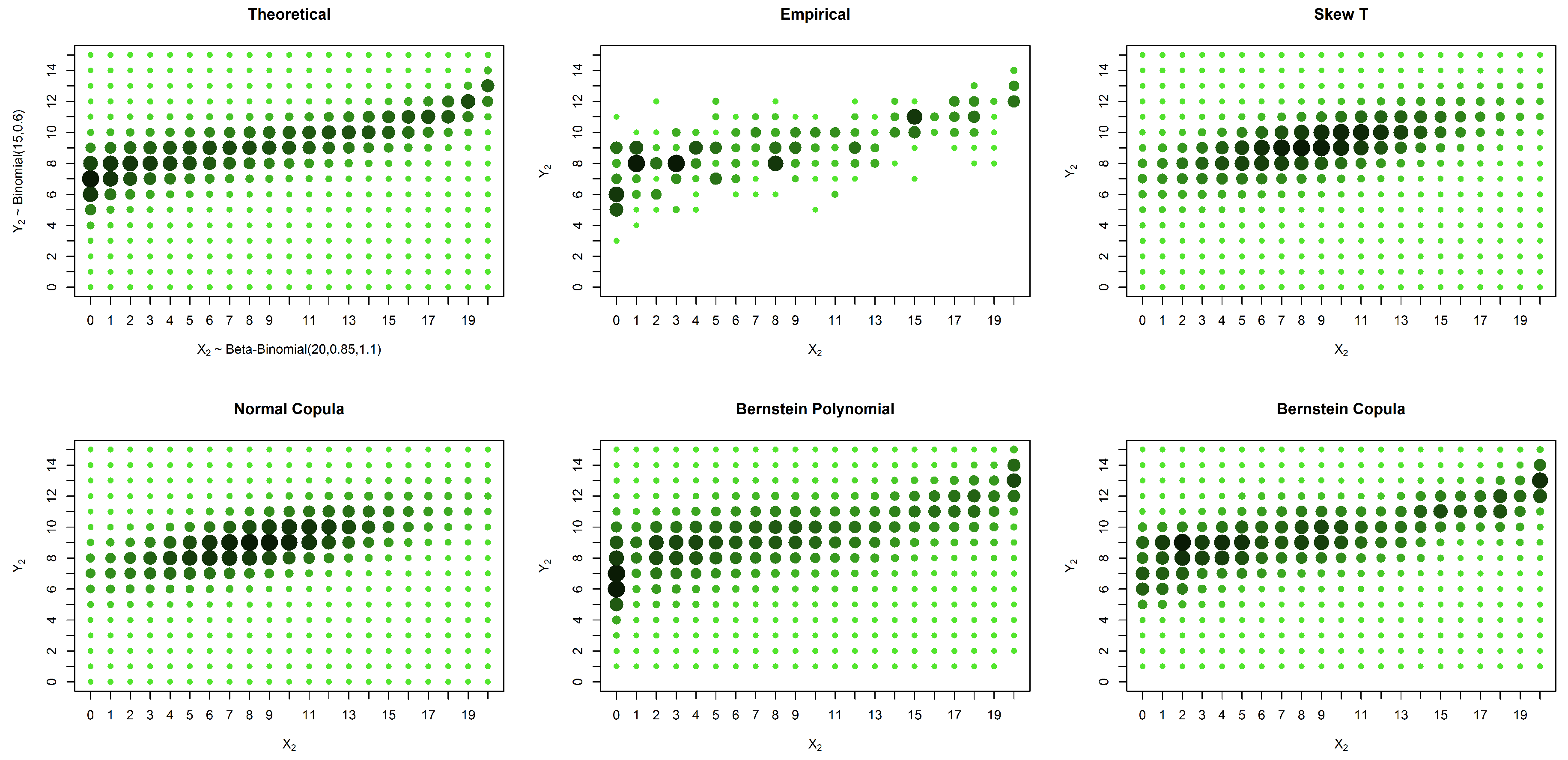
4.2. Simulated Asymmetrical Distribution
In this section, we present the simulated data for an asymmetrical distribution with margins and and a Gumbel copula with the parameter .
In the case of an asymmetrical distribution, our proposed solution yields a better estimation in all three considered cases: the case with no censored data, the case with missing data in one variable and the case with missing data in both variables. The superior performance of our approach can be observed both graphically (
Figure 5,
Figure 6 and
Figure 7) and from the calculated distances (
Table 4,
Table 5 and
Table 6). It is possible to graphically observe that the probabilities of both the smaller and larger values of
are well estimated by our method.
The new method performed better than the other presented solutions in the case of asymmetric models. It should be emphasized that the method was developed for cases with a large proportion of censored data or situations in which the number of points to be estimated is larger than the sample size.
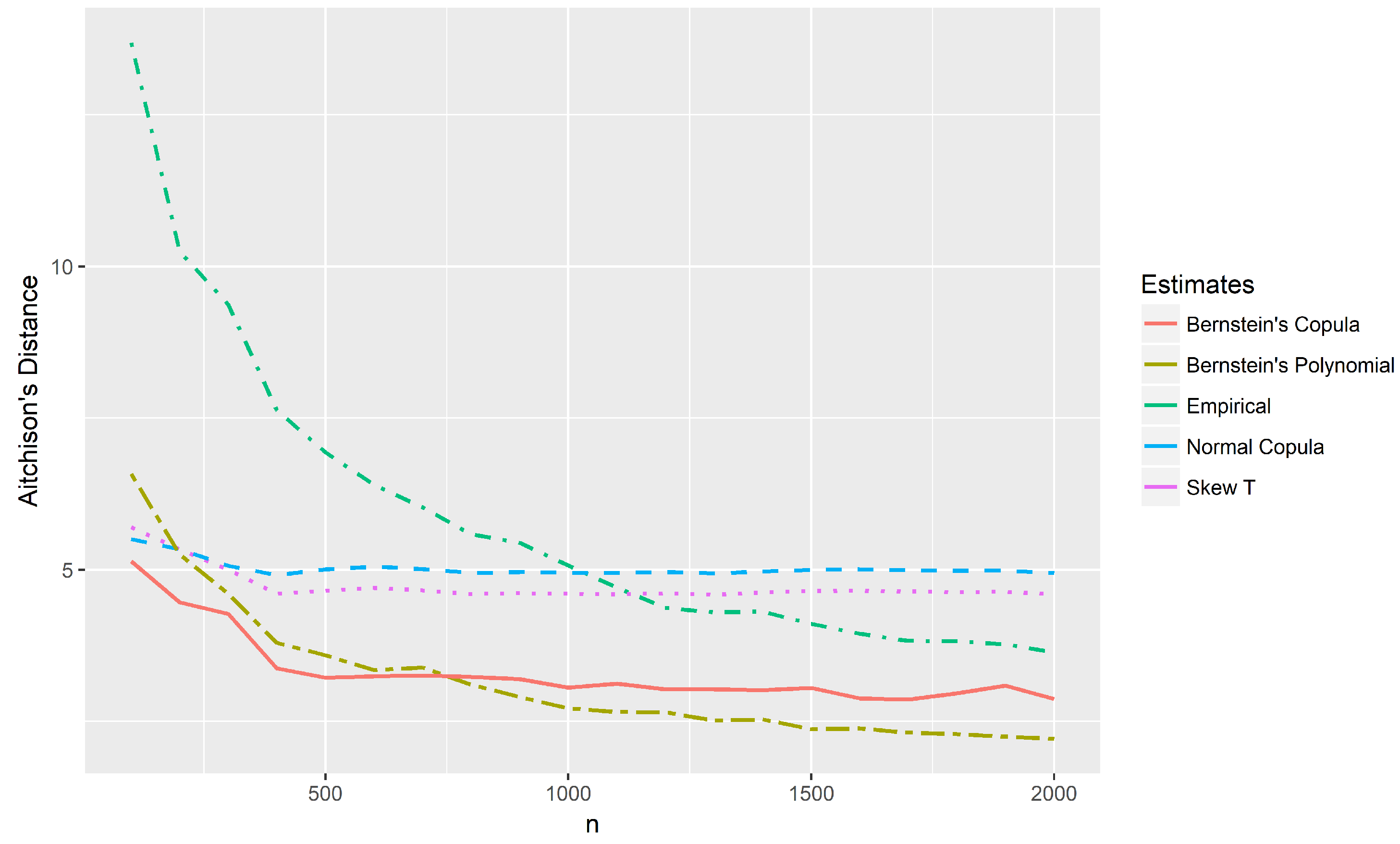
Figure 8 shows the Aitchison distances between the theoretical distribution and the estimates of the example of
Section 4.2 considering censored data in only one marginal. Sample sizes
with the same proportion of censored data of the example were considered. In this case, the support of the distribution has 336 points. Note that for small samples (
), the proposed method presents the smallest distances. Although the method was developed for small samples, it appears that its estimates converge to the theoretical distribution as
n increases. However, a detailed investigation on the asymptotic properties of the new method is needed and is the goal of a future work.
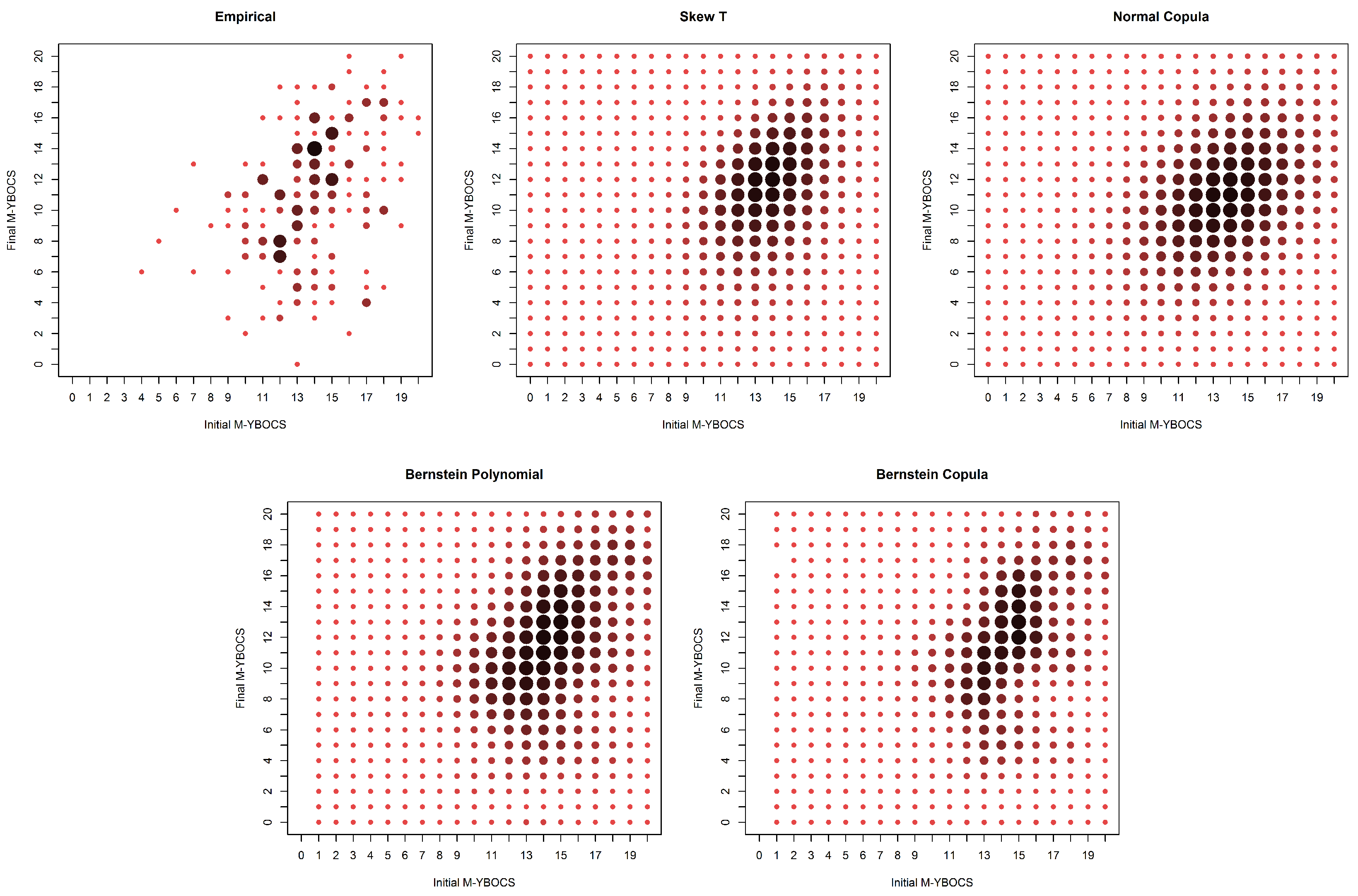
4.3. Real Data
In this section, we present the estimates for the real data described in the Introduction. The YBOCS is one of the most widely-used outcome measures in treatment studies of obsessive compulsive disorder (OCD). The total YBOCS scores comprise an integer number varying from 0–40 and intend to grade the severity of obsessive-compulsive symptoms. The total YBOCS score is the sum of two sub-scales, each ranging from 0–20, one of which measures the severity of compulsion and the other of obsession. The works in [
8,
9] propose that instead of the sum, it would be better to consider the maximum of these two sub-scales, called M-YBOCS. Thus, psychiatrists have been interested in better understanding the properties of this new scale, such as the probability distribution of M-YBOCS scores before and after patients have received some treatment for OCD.
As already mentioned in the Introduction, the dataset has 1001 observations of the scores at the initial time and only 213 at the final time. This happens because many patients drop out of treatment. The causes of drop out can be extremely different, such as a reduction in symptoms making the patient feel that he/she does not need treatment, or even worsen the symptoms, causing the patient to discredit the treatment. The small number of complete pairs in the database makes it difficult to estimate the joint distribution.
In real problems, there are few cases where the law of probability that generates the data is revealed. In such cases, a fairly common way to assess whether the proposed methods are adequate is to compare estimates with observed data. In predictive models, for example, it is common to verify some distance between predicted and observed values. In this way, we compare the distance between the estimates and the empirical probability function (which is the relative frequency of each observed point). The proposed solution yields smaller distances than do the existing approaches (
Table 7).
The estimation through the empirical distribution presents many zeros due to the small number of observations. The researchers believe that the proportion of unobserved points would decrease if the sample had fewer dropouts. In addition, they believe that common assumptions of normality or even symmetry assumptions make no sense in this case. The proposed method assigns positive probability to non-observed cells and captures the asymmetric nature of the data, which can be observed graphically in
Figure 9.
5. Conclusions
In this work, a new approach to the problem of estimating discrete bivariate distributions is presented. The procedure, which essentially consists of estimating both the marginals and the copula using Bernstein polynomials, aims at addressing three important issues: the handling of discrete bivariate data in the presence of marginal missing values (using all available information, including incomplete pairs of observations); the possibility of obtaining positive estimates for non-observed cells, thus yielding “smoother” estimated discrete distributions; and the consideration of a large variety of dependence structures between the relevant random variables. The new approach is suitable for these cases owing to its fairly unrestrictive, nonparametric nature. The use of Bernstein polynomials shows better results of the empirical distribution to estimate the marginal distribution. It is important to note that the empirical Bernstein copula produces a copula only asymptotically [
35], and other methods could be used to estimate Bernstein’s copula instead, as the one described in [
42]. Anyway, the proposed method showed reasonable estimates for the studied probability mass functions. The new method can be applied also to
p-dimensional random variables,
: both the mathematical development and the computational implementation are similar to the case
.
The new method was applied to several examples of simulated data, and according to a few typical measures of distance (between the estimated and theoretical distributions), it performed better than some of the existing solutions in cases of asymmetrical models, particularly in the presence of censored data and for cases where the number of points to be estimated is larger than the sample size. Although the method was developed for small samples, it appears that the proposed estimates converge to the theoretical distribution, but more detailed studies are still needed.
The new method was also applied to data sampled from adults diagnosed with primary obsessive-compulsive disorder. The estimate obtained by the method was appreciated by researchers in psychiatry.
While the new method has practical advantages over the presented existing alternatives, some aspects were not addressed here, namely: it will yet be necessary to further develop the new procedure in several aspects that were not addressed here: (i) the study of asymptotic properties for large sample size
n and/or for higher polynomial degree
m; (ii) a formal justification for the new procedure under a decision-theoretical approach; (iii) the development of a more rational approach to the selection of
(which could depend on
n) using the approach suggested in (ii); and (iv) the incorporation of prior knowledge, perhaps as in Petrone [
43,
44] and Petrone and Wasserman [
45], although these authors approached the problem from a univariate Bayesian perspective. These topics will be the focus of future articles.


