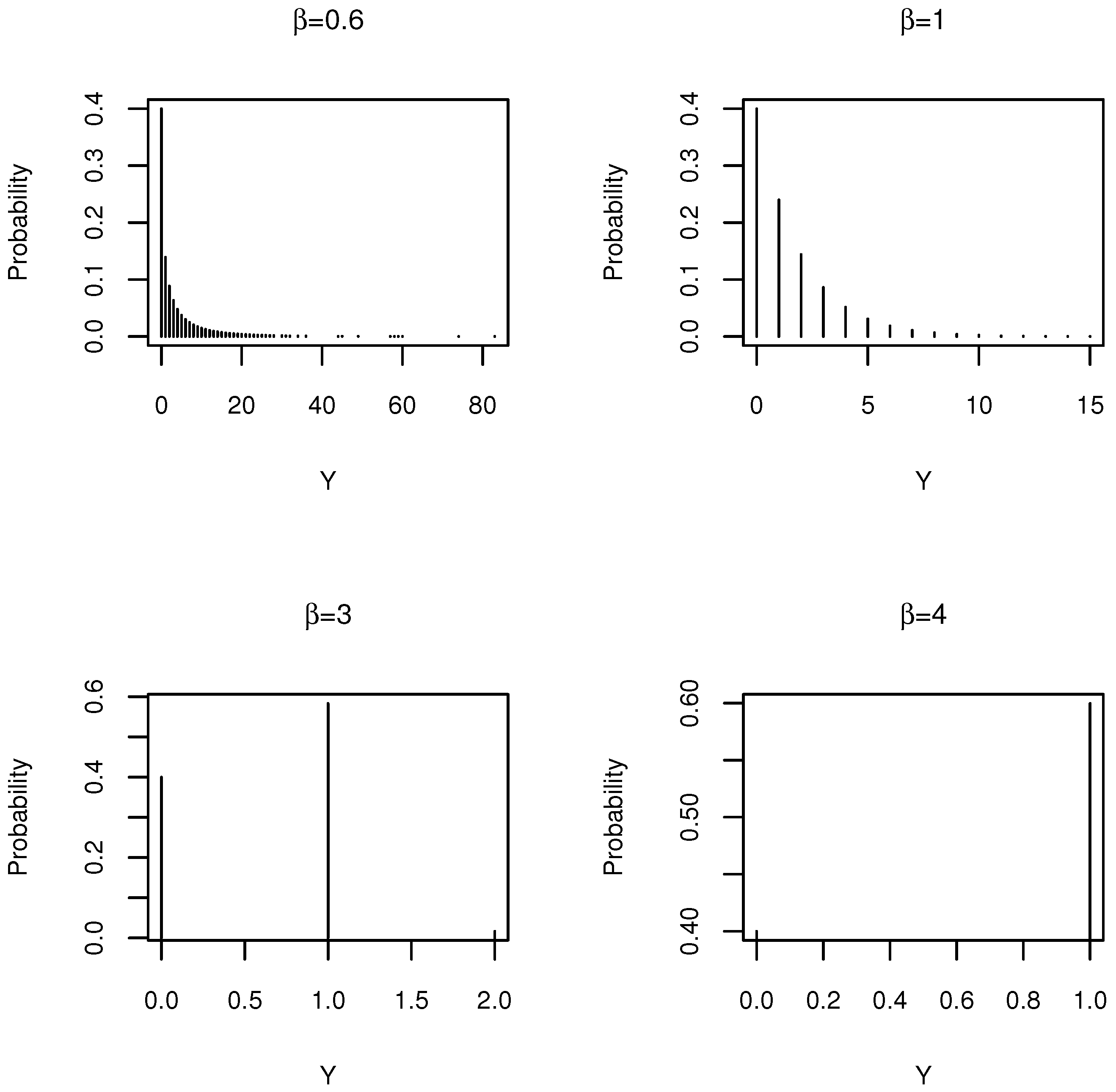
Figure 1.
The effect of on the discrete Weibull (DW) probability mass function with .
Figure 1.
The effect of on the discrete Weibull (DW) probability mass function with .
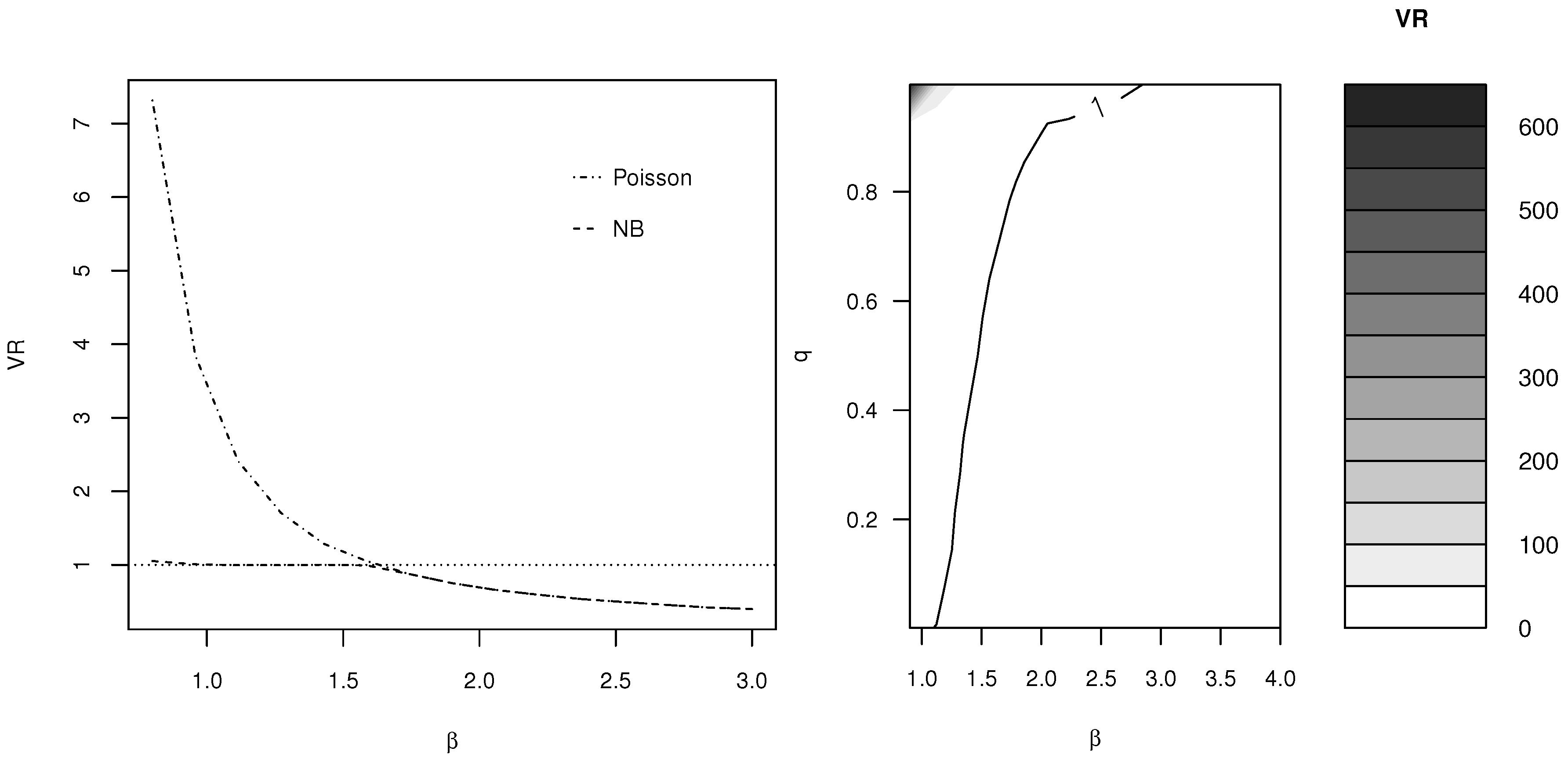
Figure 2.
Ratio of observed and theoretical variance of data simulated by . Left: ; data fitted by Poisson and negative binomial (NB) regression. Right: a range of q and values; data fitted by Poisson regression. The area below 1 corresponds to cases of underdispersion relative to Poisson regression, whereas the area above 1 corresponds to cases of overdispersion.
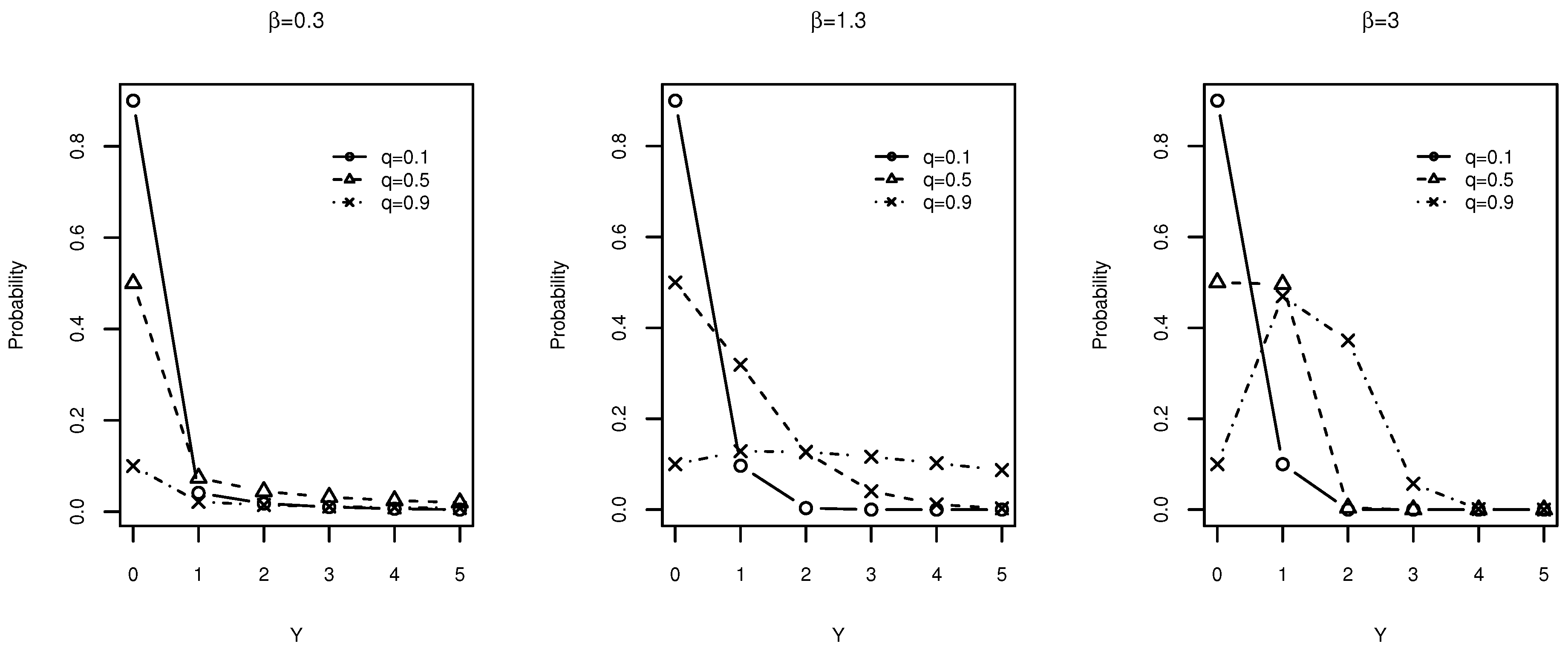
Figure 3.
Effect of q on the probability mass function of the discrete Weibull (DW) distribution for different values.
Figure 3.
Effect of q on the probability mass function of the discrete Weibull (DW) distribution for different values.
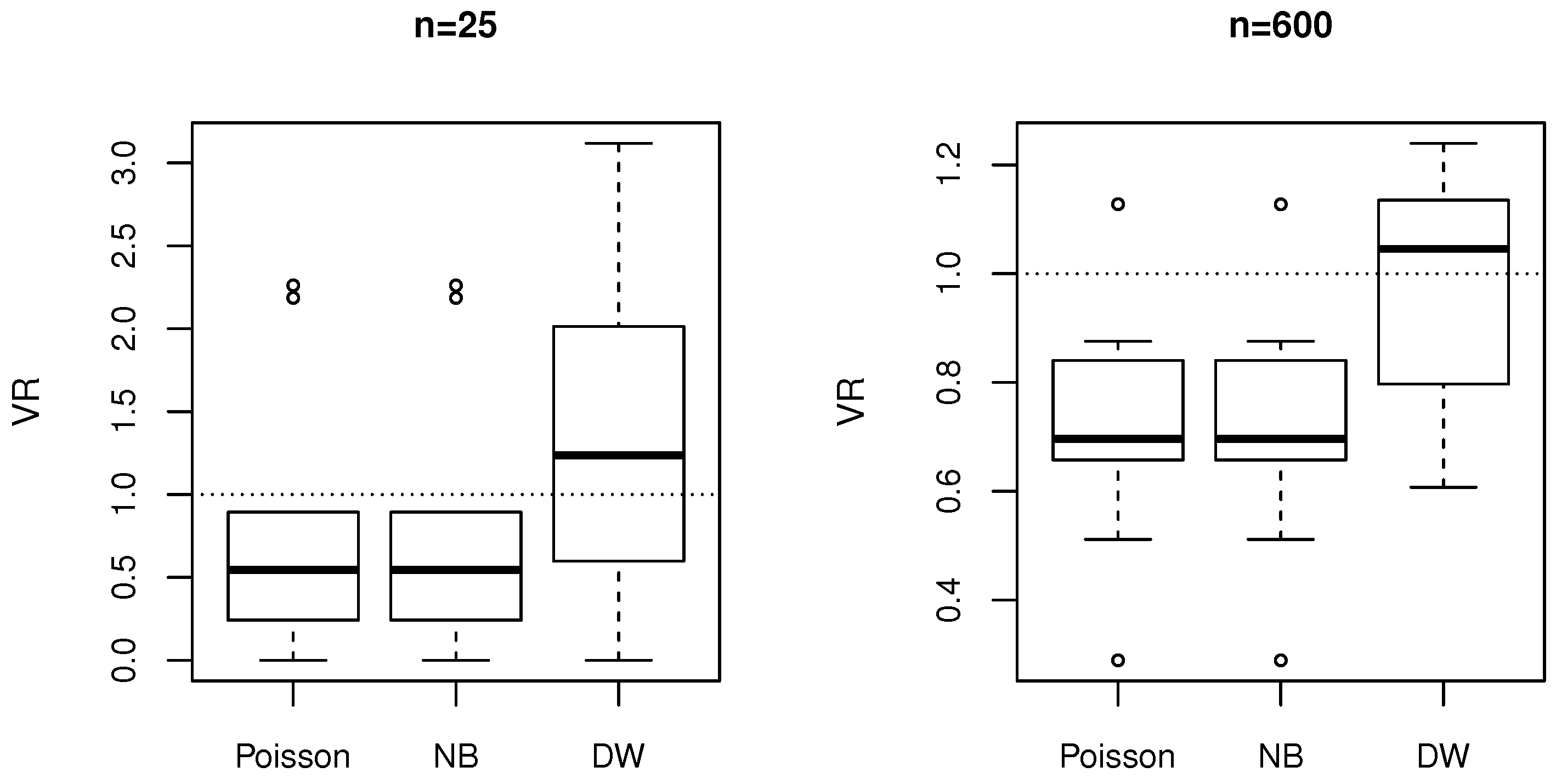
Figure 4.
Distribution of ratios of observed and theoretical conditional variance on simulated data from the discrete Weibull (DW) regression model, with the theoretical variance fitted by Poisson, negative binomial (NB) and DW models.
Figure 4.
Distribution of ratios of observed and theoretical conditional variance on simulated data from the discrete Weibull (DW) regression model, with the theoretical variance fitted by Poisson, negative binomial (NB) and DW models.
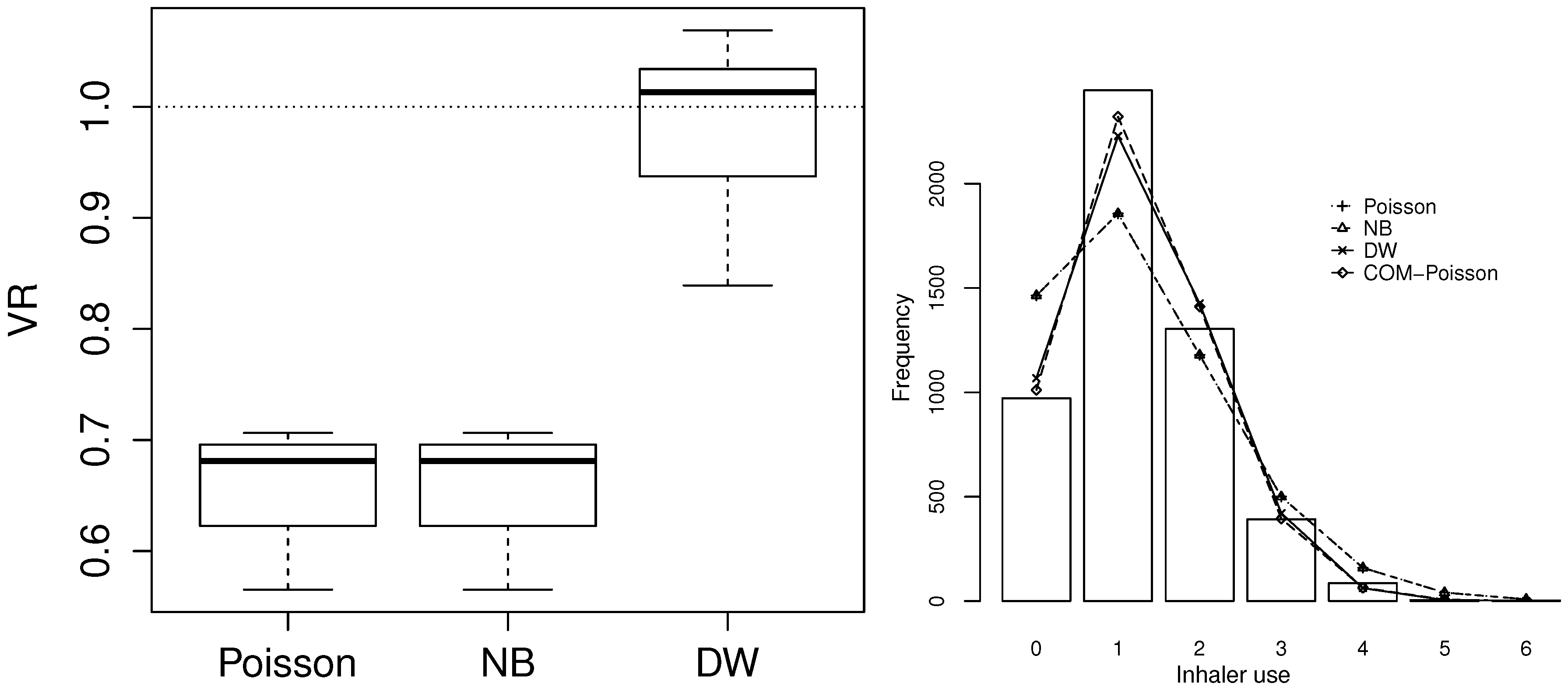
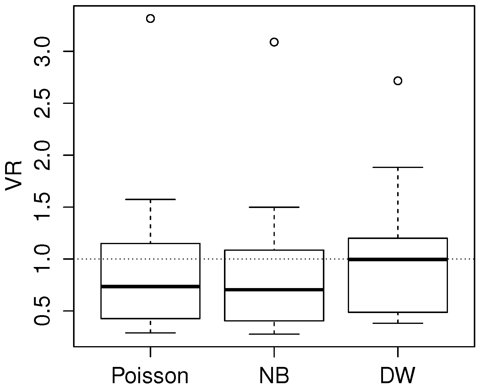
Figure 5.
Comparison of discrete Weibull (DW) regression with the other regression models on inhaler use data. Left: distribution of ratios of observed and theoretical conditional variance on the data fitted by Poisson, negative binomial (NB) and DW regression, respectively. Right: observed and expected frequencies for each model.
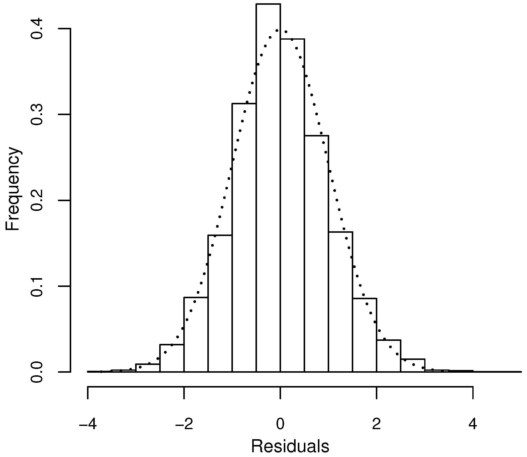
Figure 6.
Residuals analysis for inhaler use data for the discrete Weibull (DW) regression model: histogram of randomised quantile residuals with superimposed density (dotted line).
Figure 6.
Residuals analysis for inhaler use data for the discrete Weibull (DW) regression model: histogram of randomised quantile residuals with superimposed density (dotted line).
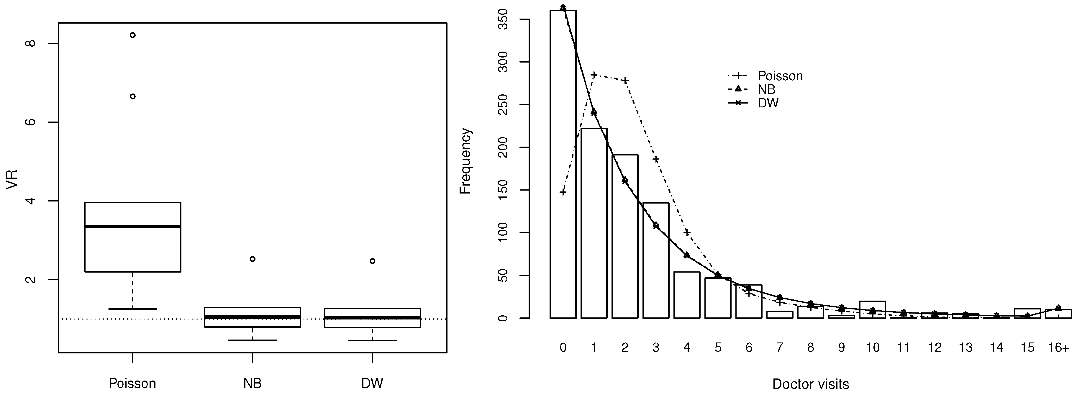
Figure 7.
Comparison of discrete Weibull (DW) with negative binomial (NB) and Poisson regression on doctor visits from German Health Survey data. Left: distribution of ratios of observed and theoretical conditional variance on the data fitted by Poisson, NB and DW regression, respectively. Right: observed and expected frequencies for each model.
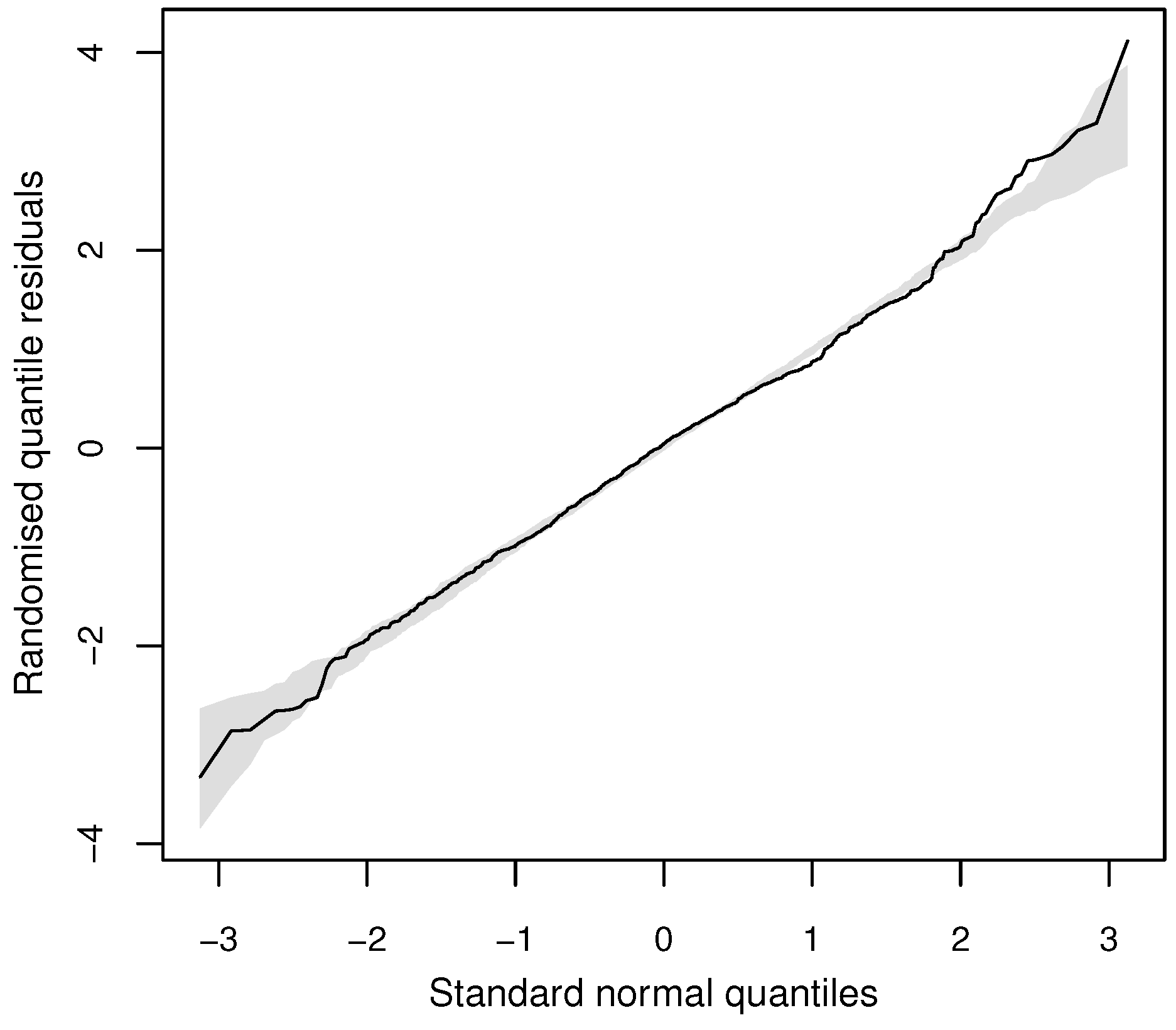
Figure 8.
Residuals analysis for doctor visits from German Health Survey data: Q-Q plot of randomised quantile residuals of the discrete Weibull (DW) regression model.
Figure 8.
Residuals analysis for doctor visits from German Health Survey data: Q-Q plot of randomised quantile residuals of the discrete Weibull (DW) regression model.
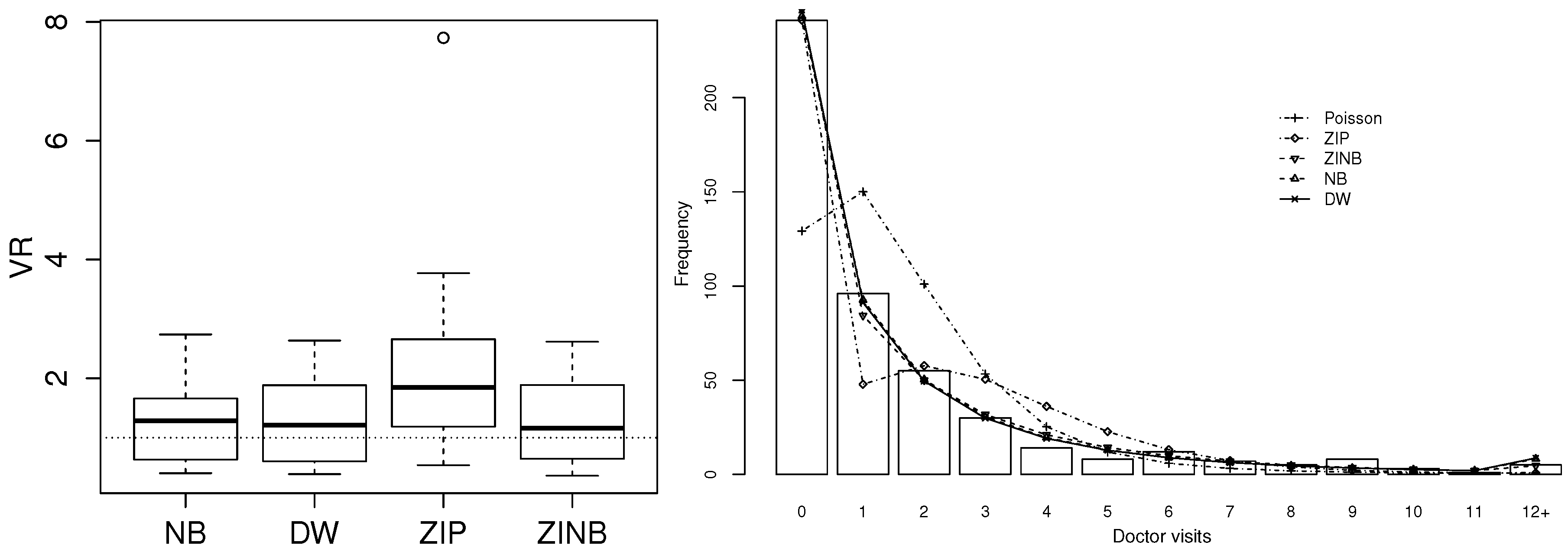
Figure 9.
Comparison of discrete Weibull (DW) regression with negative binomial (NB), zero-inflated Poisson (ZIP) and zero-inflated negative binomial (ZINB) regression on doctor visits from the United States data. Left: distribution of ratios of observed and theoretical conditional variance on the data. Right: observed and expected frequencies for each model.
Figure 10.
Distribution of ratios of observed and theoretical conditional variance on the Bids data fitted by Poisson, negative binomial (NB) and discrete Weibull (DW) regression.
Figure 10.
Distribution of ratios of observed and theoretical conditional variance on the Bids data fitted by Poisson, negative binomial (NB) and discrete Weibull (DW) regression.
Table 1.
Simulation study: discrete Weibull (DW) parameter estimates by maximum likelihood estimators (MLEs), together with bias, mean-squared error (MSE) and length of the 95% confidence interva (Cl), averaged over 1000 iterations.
Table 1.
Simulation study: discrete Weibull (DW) parameter estimates by maximum likelihood estimators (MLEs), together with bias, mean-squared error (MSE) and length of the 95% confidence interva (Cl), averaged over 1000 iterations.
| | | MLE | Bias | MSE | 95% CI Length |
|---|
| | 0.6467 | 0.1467 | 0.2932 | 1.7324 |
| 0.4908 | 0.0908 | 0.0763 | 0.8821 |
| −0.3651 | −0.0651 | 0.0241 | 0.4694 |
| 2.5924 | 0.4924 | 0.8455 | 2.4718 |
| | 0.5074 | 0.0074 | 0.009 | 0.3611 |
| 0.402 | 0.002 | 0.0021 | 0.1782 |
| −0.3033 | −0.0033 | 0.0004 | 0.0789 |
| 2.1196 | 0.0196 | 0.0086 | 0.3549 |
Table 2.
Maximum likelihood estimates, AIC and BIC from different regression models fitted to the inhaler use data.
Table 2.
Maximum likelihood estimates, AIC and BIC from different regression models fitted to the inhaler use data.
| | Humidity | Pressure | Temperature | Particles | Other | AIC | BIC |
|---|
| Poisson | −0.1125 | 4.0950 | −0.2035 | 0.0225 | — | 13915.47 | 13948.26 |
| NB | −0.1125 | 4.0950 | −0.2035 | 0.0225 | | 13917.54 | 13956.89 |
| COM–Poisson | −0.1724 | 6.2864 | −0.3128 | 0.0348 | | 13450.77 | 13490.12 |
| DW | −0.1050 | 2.6376 | −0.1735 | 0.0136 | | 13484.36 | 13523.71 |
Table 3.
Maximum likelihood estimates, AIC and BIC from different regression models fitted to the doctor visits from German Health Survey data.
Table 3.
Maximum likelihood estimates, AIC and BIC from different regression models fitted to the doctor visits from German Health Survey data.
| | Bad Health | Age | Other | AIC | BIC |
|---|
| Poisson | 1.1083 | 0.0058 | — | 5638.552 | 5653.634 |
| NB | 1.1073 | 0.0070 | | 4475.285 | 4495.394 |
| DW | 1.0068 | 0.0120 | | 4474.973 | 4495.083 |
Table 4.
Maximum likelihood estimates, AIC and BIC from different regression models fitted to doctor visits from the United States data.
Table 4.
Maximum likelihood estimates, AIC and BIC from different regression models fitted to doctor visits from the United States data.
| | Children | Access | Health | Other | AIC | BIC |
|---|
| Poisson | −0.1759 | 0.9369 | 0.2898 | — | 2179.487 | 2196.223 |
| NB | −0.1706 | 0.4197 | 0.3154 | | 1581.88 | 1602.801 |
| Zero-inflated models | | | | | | |
| Poisson | | | | | | |
| Count model | −0.1498 | 0.8053 | 0.1736 | — | 1885.813 | 1919.287 |
| Logit model | 0.0843 | −0.1048 | −0.4147 | — |
| NB | | | | | | |
| Count model | −0.1414 | 0.6491 | 0.2239 | | 1578.5 | 1616.158 |
| Logit model | 0.2465 | 1.2085 | −2.0676 | — |
| Hurdle models | | | | | | |
| Logit model | −0.1462 | 0.4252 | 0.4524 | — | — | — |
| Poisson count model | −0.1506 | 0.8143 | 0.1733 | — | 1885.808 | 1919.281 |
| NB count model | −0.1664 | 0.5404 | 0.2157 | | 1576.302 | 1613.959 |
| DW | −0.1309 | 0.3403 | 0.2758 | | 1575.796 | 1596.717 |
Table 5.
Maximum likelihood estimates, AIC and BIC from different regression models fitted to Bids data.
Table 5.
Maximum likelihood estimates, AIC and BIC from different regression models fitted to Bids data.
| | Price | Size | Regulator | Other | AIC | BIC |
|---|
| Poisson | −0.7849 | 0.0362 | 0.0547 | — | 402.2602 | 413.6054 |
| NB | −0.7824 | 0.0369 | 0.0544 | | 403.9481 | 418.1295 |
| DW | −0.6761 | 0.0552 | 0.0293 | | 395.1214 | 409.3028 |


