1. Introduction
In physics we are used to two qualitatively different time and length scales, the atomic regime and the laboratory (human scaled) regime, some 8 to 10 orders of magnitude apart. These are worlds apart although their physics must be mutually consistent.
At the atomic scale all motion is reversible and each particle must be traced individually. While at the laboratory scale we work with averaged quantities such as energy and number, from which new thermodynamic quantities such as temperature and thermodynamic pressure emerge.
A more mysterious emergent quantity is entropy. It is simply the macroscopic manifestation of microscopic degrees of freedom that cannot manifest themselves directly in day to day life. This is at the heart of the phenomenon of irreversibility which proves to be fundamentally unavoidable, even if it does not exist for much of microscopic physics.
On accepting these new properties, we no longer need to know about the individual particles. We do not need their existence, and can complete our description entirely among the macroscopic variables. The scales from which the laboratory regime emerged can be thus ignored. Thermodynamically speaking the thermodynamic system variables form a closed group just like the microscopic quantities do, but are related through functions rather than dynamical equations. Thus in the process we lost some variables and concepts but gained others, ones that could not be fully anticipated knowing only the microscopic world.
We are now interested in making a further similar jump of 8 to 10 orders of magnitude to extremely long time scales (“slow time”) and size scales in order to investigate which, if any, of our traditional thermodynamic quantities survive [
1,
2]. Total mass and total particle number do, just like they did from atomic to laboratory scale. In the next sections we will see that some quantities persist, possibly with new components, while others no longer have meaning.
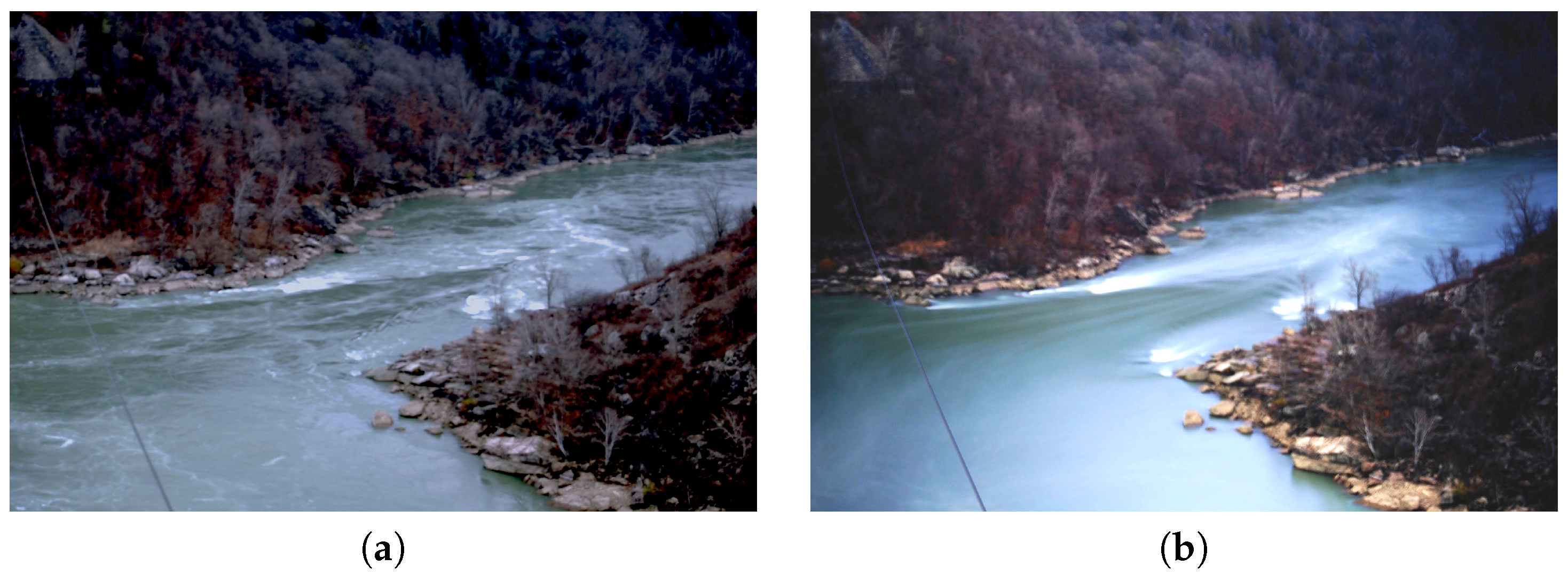
A small step in the direction of slow time may be seen in
Figure 1 which shows the same scene in a normal short time exposure (
Figure 1a) and in a somewhat longer time exposure (
Figure 1b). A lot of unimportant “noise” is absent in the longer exposure while instead classical fluid features like standing waves, stream lines and vortices become fully apparent.
2. No Wind
As a simple illustration, let’s look at the probability density function,
p, that defines the velocity distribution of a small volume of gas with rest velocity
u and temperature
T, which in one dimension is
where
m is the particle mass, and
k Boltzmann’s constant. On a long timescale this rest velocity (wind) will also vary, so let’s assume that this also follows a Gaussian distribution with standard deviation
. The convolution of these two distributions is physically distinct from the classical distribution, but mathematically still a Maxwellian form [
1],
with zero rest velocity and a non-classical temperature,
The second term can most simply be thought of as thermalization of mechanical wind, i.e., its random magnitude and direction. This is the slow time version of the rapid Brownian motion which also averages out directed mechanical motion to thermal energy.
We see two important lessons here: (i) On the long timescale the velocity distribution is still Maxwellian in form; and (ii) the concept of temperature, with all its ramifications, is in a sense unchanged, but its physical meaning differs to include the fluctuations of wind which are no longer discernible at this long timescale. However the velocity concept remains intact.
To get an idea of the significance of this extra term in Equation (
3), set the width of wind fluctuations
as representative for air at
K. Then the extra contribution amounts to about
K. This is for most practical purposes insignificant, but for other than material flows it could be important.
3. No Temperature
The aim is to reveal what the Maxwellian distribution becomes in the slow time limit, i.e., the
“slow time Maxwellian". This is needed prior to slow time analogues to fluid mechanics or thermodynamics. Some preliminary conceptual ideas have been published in [
3,
4]. While we take an approach similar to classical statistical mechanics, ours is more speculative because, unlike classical statistical mechanics, only one regime is known a priori.
Space scales accompany timescales. If a collection of particles have a characteristic speed, their ability to interact with surrounding particles is limited spatially when given a particular timescale. Groups of particles beyond this characteristic distance are independent, while on longer timescales they are not. Thus to consider the slow time behavior one must consider a box with space coordinates and time. The box only represents the sampling space, allowing particles to pass freely.
To ensure one is not just constructing an ensemble of particles that will recover the classical Maxwellian behavior for the laboratory regime, we imagine that the box is composed of small cells each having its own local statistics defined by a local Maxwellian, with a temperature T and a rest velocity u. We then proceed with distributions in u and T to capture the distribution of the entire space-time box. This picture treats local velocity u and temperature T as representing fluctuations in local particle states within cells. Since the slow time regime treats the box as the limit of resolution, the distribution of the box becomes the observed particle distribution, which is the composition of the individual Maxwellians within it.
As our first example above we considered the effect of a fluctuating velocity u about 0 for fixed T. As u is not only the rest frame velocity, but becomes the wind of fluid mechanics, there is a trade off between wind and temperature on long timescales. The new temperature appeared as it normally does in equilibrium, but for a slow time equilibrium. Thus for fixed T a slow time ideal gas has a revised temperature which emerges in velocity moments generating all of the standard expressions in place of T. Wind becomes thermalized not by process but by resolution.
However, things are not so neat when temperatures fluctuate, because temperature also appears in the normalization of the distribution. As above for wind, we make the same considerations about temperature and its variations over time (e.g., day/night, summer/winter) by allowing it to vary with a Gaussian distribution. This convolution is no longer Maxwellian but takes the form
where
is the standard deviation of the temperatrure fluctuations around a mean
.
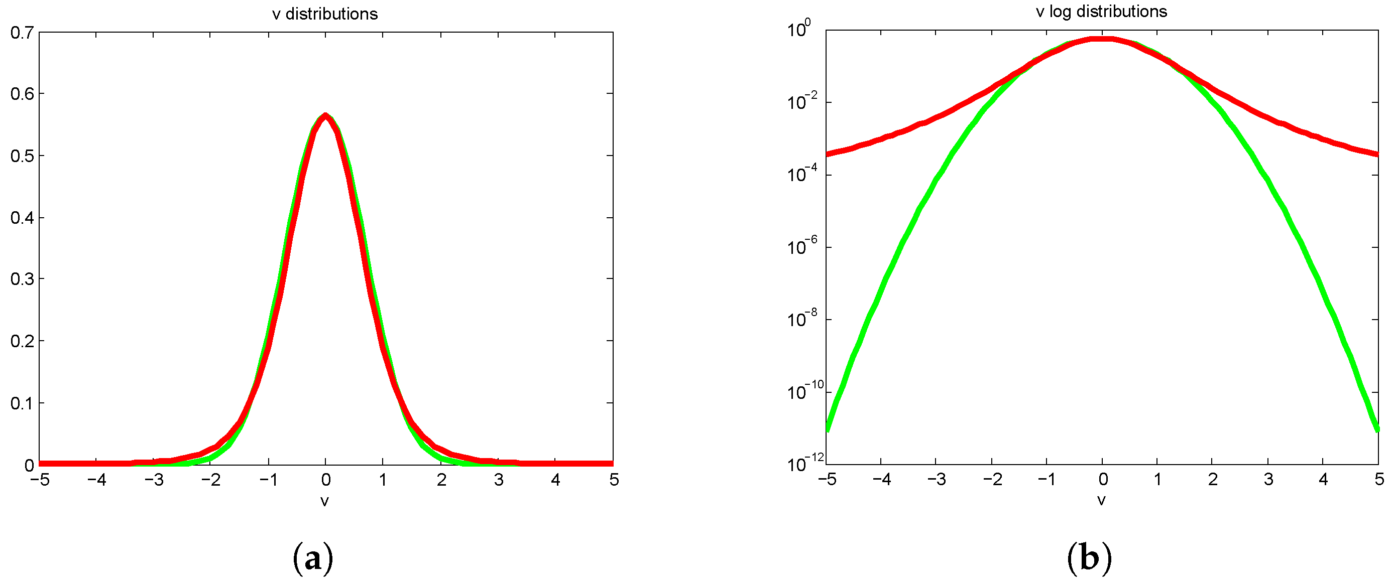
At first sight it might look like an ordinary velocity distribution at a certain temperature (
Figure 2a), but on a logarithmic scale (
Figure 2b) it is quite obvious that the wings do not decay in a Gaussian fashion, they are polynomial. It is a distinctive hybrid with a Gaussian core and heavy (polynomial) tails. Not only does that mean that the concept of temperature as we are used to it no longer persists on long timescales, but also the distribution is not normalizable.
We yet have to find out the full range of which ones of our usual laboratory scale thermodynamic variables survive the transition to long timescales.
4. Linking Phenomenology to Mathematics: Closure
If one aims to go further than simply describing unexpected and novel phenomena by actually searching for distinct regimes that we have no a priori experience with, mathematical structures provide strong constraints on what the possibilities can be. What constitutes a distinct regime hangs on whether the long-time and space structures can exist without direct reference to the short-time and space one from which it emerges. That is, can the underlying structures be ignored while being consistent with the underlying structure. Mathematically the equations in the new variables are then said to be closed.
If closure cannot be established, one must question the physical legitimacy of the new regime. This is the theoretical dilemma of the Navier Stokes equations which are presumed to capture turbulent flows, but averages over them have resisted producing closed equations without resorting to unphysical ad hoc assumptions.
This issue is not solely one of differential equations either. The existence of averaged functions arising from underlying functions is similar, though simpler [
3] to understand: just because an explicit function exists for two variables does not mean that a function also exists between their averages. This goes so strongly against common thinking that a simple illustration was done in [
3], which we demonstrate here as it is pertinent to the underlying thinking of this paper because functions are a natural context for thermodynamical thinking.
Suppose that there are two families of functions
and
in parameters
w and
v, respectively. Define an average
which is a functional of
h. Now let two variables,
x and
y, be simply related by
. If in turn
is drawn
only from the first family (i.e.,
) then
Similarly, if
is drawn
only from the second family (i.e.,
) instead,
In both scenarios the averaged variables are indeed related by a function. The underlying parameter disappears in the integration, which defines which member of the family is in play. In each case, however, the particular family member can be ignored. One needs only know to predict .
Now suppose instead that
is given by
and
. In this case
does not predict
uniquely: they are not related by a function. To determine
from
the underlying problem must be consulted as well. The underlying regime cannot be ignored. The problem is not closed under (
5). Broader classes of functions for
increases the need to consult the underlying regime to determine
.
This is only a simplistic example for functions. Underlying regimes in differential equations increase the difficulties with this issue as the Navier Stokes equations perfectly illustrate.
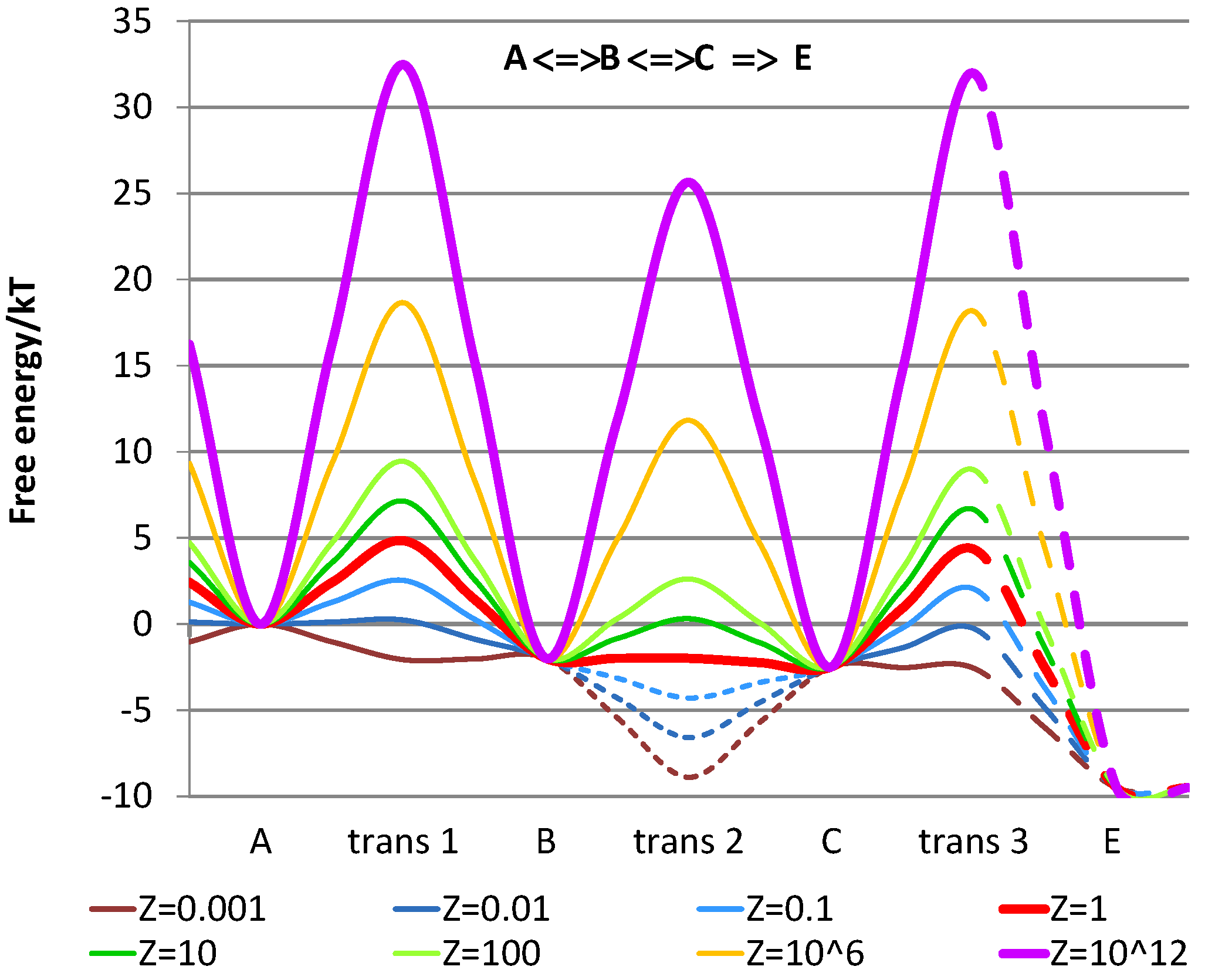
5. Resolution of Chemical Reactions
In the next few sections we will give examples of known situations where the timescale makes a decisive influence on the measured results. Going all the way to slow time we expect even more striking differences. Consider the chemical reaction
, i.e., the conversion of
A to
E through the intermediate rapid rearrangement
[
5]. The free energy landscape for this reaction goes through 3 transition states with energies given by expressions like
where
r is the reaction rate constant for the particular component and
Z, in the Eyring-Polanyi formulation [
6], is the reaction attempt frequency (collision rate). A reinterpretation of this means that
is the time resolution or observation time of the experiment.
As illustrated in
Figure 3, this observation time
has a major effect on the perceived transition state barrier varying from
or more at molecular collision frequencies to zero or even less at observation times of 1 s and more. In other words, even at quick manual laboratory handling times the rearrangement
is perceived as instantaneous without any barrier while at even slower experimental times (about 2 min and above) there is seemingly no barrier between the end products
A and
E. Once again, the timescale of the observation has a decisive effect on the apparent phenomena seen, even on a more moderate scale than 10 orders of magnitude.
6. Eigentimes
Another aspect of what we observed in the previous section is the cascade of eigentimes often encountered in atomic physics, in particular in beam-foil spectroscopy [
7]. The excitation decay signature often looks like
Figure 4 in which the separation of timescales between different decay mechanisms is particularly visible in a semilog plot (
Figure 4b). The fastest decay follows an exponential form before the second fastest have changed noticeably, and eventually only the slowest decay remains. With a clear separation of timescales one can study several reactions in a single run.
In biology there is extensive empirical evidence that the metabolic rate of an organism scales with the
power of the organism’s mass
M, where
is between
and
. The
relates to the dimensional ratio of the organism’s surface to its volume while the
stems from the flow-optimal branching ratio for a supply chain [
8].
General optimization results from physics indicate that maximum efficiency of a process, in the sense of minimum overall entropy production, is achieved when the rate of entropy production is constant over time. However, this is not in ordinary clock time but on an eigentime scale intrinsic to the system [
9]. In general this eigentime may vary in terms of clock time from system to system as well as with varying conditions. The exponent
above implies a physiological eigentime
which scales with the exponent
, i.e., typically
. This means that typical times for a mouse, e.g., life span, 1/heart rate, 1/breathing frequency, are consistently much shorter than for an elephant. This relationship implies that all organisms produce entropy at the same intrinsic rate, fulfilling a necessary condition for maximum efficiency, and are thus furthermore equally efficient
on their physiological eigentime scales [
9].
7. Evolutionary Modeling
One of the more successful models for evolution, truely a slow time process, is the Tangled Nature Model [
10]. It is a model with long periods of apparent stability, interrupted by sudden major changes, “quakes”. Those were e.g., the Cambrian explosion about 540 Myr ago when earth’s atmosphere got poisoned by oxygen and opened the way for all current breathing organisms, and the meteor impact some 65 Myr ago which killed the dinosaurs and many other species, opening the field for mammals. Such glass-like models have many timescales and an ever growing rate of entropy production at the same time as an increase of system order. The increase of order appears through the quakes while the finer optimizations develop during the quiescent periods. The dominant relaxation time increases exponentially, i.e., on logarithmic clock time. While one frequently uses simplified models, possibly without the proper behavior at large distances, locally, such local models are not adequate for the far larger reaches of slow time. Actually, the infrequent but disruptive evolution components become the decisive ones in the long run.
8. Discussion
A key issue in any thermodynamic description is, what is a state? As we have seen above, the answer generally depends on the timescale over which we are looking
and the accuracy we desire. At low accuracy we cannot or do not care to distinguish finer details which means e.g., that we count all hydrogen molecules regardless of excitation. This results in fewer “states” but each one with a larger entropy. We might also be focused on a time evolving system where a certain graininess is required to distinguish one “state” from another. In [
11] we have made the criterion for when a “state” is distinguishable concrete:
i.e., when distances
ℓ in configuration space are small compared to the gradients in local thermodynamic intensities,
, divided into the local measured intensity. Correspondingly, two quantum states are distinguishable when the thermodynamic distance between them is larger than one fluctuation [
12].
Based on this criterion we see that in general local temperature (let alone global temperature) does not exist in a dynamical system on long timescales, whereas entropy may still exist as long as entropy is defined as an additive quantity; that goes for all thermodynamic extensities, such as energy, as well. Heat, being disordered motion, is more questionable since the time and length scales for the disorder become important.
A further complication to when we may talk about a state and its possible evolution is whether it is given entirely in the variables associated with that time and length scale, i.e., whether those variables form a closed set, as already indicated in the introduction. A “state” is not allowed to depend on “deeper” variables or on the dynamics at that lower level. Another way of putting this is that the dynamics of a set of (microscopic) variables and of their (macroscopic) averages are not necessarily the same. This issue though subtle is crucial to the existence of other regimes.
There is always the danger that the notion of different timescales is something artificially imposed rather than an emergent property of the phenomenon in question. For example, one can impose the perturbation theory method of multiple timescales on differential equations generally, even if no other timescale regimes actually exist. There are of course differential equations where more than one timescale is indeed an inherent property of the solutions, which can thus be treated profitably as a composition of these different regimes. The issue of closure provides some clarity to this question. This will be explored more thoroughly in future work.
In this paper we have given the first examples of one variable (wind) which persists in slow time and one (temperature) which does not. Future work will need to develop a more complete list of such variables and the way they interact. New slow time physical laws will emerge while some of our traditional laws will disappear. These derivations will then have to be compared with observations for slow processes like biological evolution as well as astronomical evolution. The possibilities are endless.


