Computing Entropies with Nested Sampling

Abstract

The Shannon entropy, and related quantities such as mutual information, can be used to quantify uncertainty and relevance. However, in practice, it can be difficult to compute these quantities for arbitrary probability distributions, particularly if the probability mass functions or densities cannot be evaluated. This paper introduces a computational approach, based on Nested Sampling, to evaluate entropies of probability distributions that can only be sampled. I demonstrate the method on three examples: a simple Gaussian example where the key quantities are available analytically; (ii) an experimental design example about scheduling observations in order to measure the period of an oscillating signal; and (iii) predicting the future from the past in a heavy-tailed scenario.

1. Introduction

If an unknown quantity x has a discrete probability distribution $p\left(x\right)$, the Shannon entropy [1,2] is defined as

$$\begin{array}{cc}\hfill H\left(x\right)& =-\sum _{x}p\left(x\right)logp\left(x\right),\hfill \end{array}$$

(1)

where the sum is over all of the possible values of x under consideration. The entropy quantifies the degree to which the issue “what is the value of x, precisely?” remains unresolved [3]. More generally, the ‘Kullback–Leibler divergence’ quantifies the degree to which a probability distribution $p\left(x\right)$ departs from a ‘base’ or ‘prior’ probability distribution $q\left(x\right)$ [4,5]:

$$\begin{array}{cc}\hfill D_{\mathrm{KL}}\left(p\left|\right|q\right)& =\sum _{x}p\left(x\right)log\left[\frac{p\left(x\right)}{q\left(x\right)}\right].\hfill \end{array}$$

(2)

If $q\left(x\right)$ is taken to be uniform, this is equivalent (up to an additive constant and a change of sign) to the Shannon entropy $H\left(x\right)$. With the negative sign reinstated, Kullback–Leibler divergence is sometimes called relative entropy, and is more fundamental than the Shannon entropy [4]. However, this paper focuses on the Shannon entropy for simplicity and because the resulting algorithm calculates the expected value of a log-probability.

The Shannon entropy can be interpreted straightforwardly as a measure of uncertainty. For example, if there is only one possible value that has a probability of one, $H\left(x\right)$ is zero. Conventionally, $0\times log0$ is defined to be equal to ${lim}_{x\to 0^{+}}(xlogx)$, which is zero; i.e., ‘possibilities’ with probability zero do not contribute to the sum. If there are N possibilities with equal probabilities $1/N$ each, then the entropy is $H\left(x\right)=log\left(N\right)$. If the space of possible x-values is continuous so that $p\left(x\right)$ is a probability density function, the differential entropy

$$\begin{array}{cc}\hfill H\left(x\right)& =-\int p(x)logp(x)dx\hfill \end{array}$$

(3)

quantifies uncertainty by generalising the log-volume of the plausible region, where volume is defined with respect to $dx$. Crucially, in continuous spaces, the differential entropy is not invariant under changes of coordinates, so any value given for a differential entropy must be understood with respect to the coordinate system that was used. Even in discrete cases, using the Shannon entropy assumes that each possibility contributes equally when counting possibilities—if this is inappropriate, the relative entropy should be used.

Entropies, relative entropies, and related quantities tend to be analytically available only for a few families of probability distributions. On the numerical side, if $logp\left(x\right)$ can be evaluated for any x, then simple Monte Carlo will suffice for approximating $H\left(x\right)$. On the other hand, if $p\left(x\right)$ can only be sampled but not evaluated (for example, if $p\left(x\right)$ is a marginal or conditional distribution, or the distribution of a quantity derived from x), then this will not work. Kernel density estimation or the like e.g., [6] may be effective in this case, but is unlikely to generalise well to high dimensions.

This paper introduces a computational approach to evaluating the Shannon entropy $H\left(x\right)$ of probability distributions that can only be sampled using Markov Chain Monte Carlo (MCMC). The key idea is that Nested Sampling can create an unbiased estimate of a log-probability, and entropies are averages of log-probabilities.

Notation and Conventions

Throughout this paper, I use the compact ‘overloaded’ notation for probability distributions favoured by many Bayesian writers [7,8], writing $p\left(x\right)$ for either a probability mass function or a probability density function, instead of the more cumbersome $P(X=x)$ or $f_X\left(x\right)$. In the compact notation, there is no distinction between the ‘random variable’ itself (X) and a similarly-named dummy variable (x). Probability distributions are implicitly conditional on some prior information, which is omitted from the notation unless necessary. All logarithms are written log and any base can be used, unless otherwise specified (for example by writing ln or ${log}_{10}$). Any numerical values given for the value of specific entropies are in nats, i.e., the natural logarithm was used.

Even though the entropy is written as $H\left(x\right)$, it is imperative that we remember that it is not a property of the value of x itself, but a property of the probability distribution used to describe a state of ignorance about x. Throughout this paper, $H\left(x\right)$ is used as notation for both Shannon entropies (in discrete cases) and differential entropies (in continuous cases). Which one it is should be clear from the context of the problem at hand. I sometimes write general formulae in terms of sums (i.e., as they would appear in a discrete problem), and sometimes as integrals, as they would appear in a continuous problem.

2. Entropies in Bayesian Inference

Bayesian inference is the use of probability theory to describe uncertainty, often about unknown quantities (‘parameters’) $\mathit{\theta }$. Some data $\mathit{d}$, initially unknown but thought to be relevant to $\mathit{\theta }$, is obtained. The prior information leads the user to specify a prior distribution $p\left(\mathit{\theta }\right)$ for the unknown parameters, along with a conditional distribution $p\left(\mathit{d}\right|\mathit{\theta })$ describing prior knowledge of how the data is related to the parameters (i.e., if the parameters were known, what data would likely be observed?). By the product rule, this yields a joint prior

$$\begin{array}{cc}\hfill p(\mathit{\theta },\mathit{d})& =p\left(\mathit{\theta }\right)p\left(\mathit{d}\right|\mathit{\theta }),\hfill \end{array}$$

(4)

which is the starting point for Bayesian inference [5,9]. In practical applications, the following operations are usually feasible and have a low computational cost:

• Samples can be generated from the prior $p\left(\mathit{\theta }\right)$;
• Simulated datasets can be generated from $p\left(\mathit{d}\right|\mathit{\theta })$ for any given value of $\mathit{\theta }$;
• The likelihood, $p\left(\mathit{d}\right|\mathit{\theta })$, can be evaluated cheaply for any $\mathit{d}$ and $\mathit{\theta }$. Usually, it is the log-likelihood that is actually implemented, for numerical reasons.

Throughout this paper, I assume that these operations are available and inexpensive.

2.1. The Relevance of Data

The entropy of the prior $p\left(\mathit{\theta }\right)$ describes the degree to which the question “what is the value of $\mathit{\theta }$, precisely?” remains unanswered, while the entropy of the joint prior $p(\mathit{\theta },\mathit{d})$ describes the degree to which the question “what is the value of the pair $(\mathit{\theta },\mathit{d})$, precisely?” remains unanswered. The degree to which the question “what is the value of $\mathit{\theta }$?” would remain unresolved if $\mathit{d}$ were resolved is given by the conditional entropy

$$\begin{array}{cc}\hfill H\left(\mathit{\theta }\right|\mathit{d})& =-\sum _{\mathit{d}}p\left(\mathit{d}\right)\sum _{\mathit{\theta }}p\left(\mathit{\theta }\right|\mathit{d})logp\left(\mathit{\theta }\right|\mathit{d}),\hfill \end{array}$$

(5)

which is the expected value of the entropy of the posterior, averaged over all possible datasets that might be observed.

One might wish to compute $H\left(\mathit{\theta }\right|\mathit{d})$, perhaps to compare it to $H\left(\mathit{\theta }\right)$ and quantify how much might be learned about $\mathit{\theta }$. This would be difficult because the expression for the posterior distribution

$$\begin{array}{cc}\hfill p\left(\mathit{\theta }\right|\mathit{d})& =\frac{p\left(\mathit{\theta }\right)p\left(\mathit{d}\right|\mathit{\theta })}{p\left(\mathit{d}\right)}\hfill \end{array}$$

(6)

contains the marginal likelihood:

$$\begin{array}{cc}\hfill p\left(\mathit{d}\right)& =\sum _{\mathit{\theta }}p\left(\mathit{\theta }\right)p\left(\mathit{d}\right|\mathit{\theta }),\hfill \end{array}$$

(7)

also known as the ‘evidence’, which tends to be computable but costly, especially when the summation is replaced by an integration over a high-dimensional parameter space.

It is important to distinguish between $H\left(\mathit{\theta }\right|\mathit{d})$ and the entropy of $\mathit{\theta }$ given a particular value of $\mathit{d}$, which might be written $H\left(\mathit{\theta }\right|\mathit{d}={\mathit{d}}_{\mathrm{obs}})$ (‘obs’ for observed). The former measures the degree to which one question answers another ex ante, and is a function of two questions. The latter measures the degree to which a question remains unresolved after conditioning on a specific statement (ex post), and is a function of a question and a statement.

2.2. Mutual Information

The mutual information is another way of describing the relevance of the data to the parameters. Its definition, and relation to other quantities, is

$$\begin{array}{cc}\hfill I(\mathit{\theta };\mathit{d})& =\sum _{\mathit{\theta }}\sum _{\mathit{d}}p(\mathit{\theta },\mathit{d})log\left[\frac{p(\mathit{\theta },\mathit{d})}{p\left(\mathit{\theta }\right)p\left(\mathit{d}\right)}\right]\hfill \end{array}$$

(8)

$$\begin{array}{c}=H\left(\mathit{\theta }\right)+H\left(\mathit{d}\right)-H(\mathit{\theta },\mathit{d})\hfill \end{array}$$

(9)

$$\begin{array}{c}=H\left(\mathit{d}\right)-H\left(\mathit{d}\right|\mathit{\theta })\hfill \end{array}$$

(10)

$$\begin{array}{c}=H\left(\mathit{\theta }\right)-H\left(\mathit{\theta }\right|\mathit{d}).\hfill \end{array}$$

(11)

The mutual information can also be written as the expected value (with respect to the prior over datasets $p\left(\mathit{d}\right)$) of the Kullback–Leibler divergence from prior to posterior:

$$\begin{array}{cc}\hfill I(\mathit{\theta };\mathit{d})& =\sum _{\mathit{d}}p\left(\mathit{d}\right)D_{\mathrm{KL}}\left(p\left(\mathit{\theta }\right|\mathit{d}\left)\right|\left|p\right(\mathit{\theta })\right).\hfill \end{array}$$

(12)

In terms of the prior, likelihood, and evidence, it is

$$\begin{array}{cc}\hfill I(\mathit{\theta };\mathit{d})& =\sum _{\mathit{\theta }}\sum _{\mathit{d}}p\left(\mathit{\theta }\right)p\left(\mathit{d}\right|\mathit{\theta })\left[logp\left(\mathit{d}\right|\mathit{\theta })-logp(\mathit{d})\right],\hfill \end{array}$$

(13)

i.e., the mutual information is the prior expected value of the log likelihood minus the log evidence. As with the conditional entropy, the computational difficulty appears in the form of the log evidence, $logp\left(\mathit{d}\right)=log\left({\sum }_{\mathit{\theta }}p\left(\mathit{\theta }\right)p\left(\mathit{d}\right|\mathit{\theta })\right)$, which must be evaluated or estimated for many possible datasets.

For experimental design purposes, maximising the expected amount of information obtained from the data is a sensible goal. Formally, either maximising $I(\mathit{\theta };\mathit{d})$ or minimising $H\left(\mathit{\theta }\right|\mathit{d})$ will produce the same result because the prior $p\left(\mathit{\theta }\right)$ does not vary with the experimental design. Reference priors [10] also maximise $I(\mathit{\theta };\mathit{d})$ but vary the prior $p\left(\mathit{\theta }\right)$ in the maximisation process while keeping the experimental design fixed.

3. Nested Sampling

Nested Sampling (NS), introduced by Skilling [11], is an algorithm whose aim is to calculate the evidence

$$\begin{array}{cc}\hfill p\left(\mathit{\theta }\right)& =\int p(\mathit{\theta })p(\mathit{d}|\mathit{\theta })d\mathit{\theta },\hfill \end{array}$$

(14)

or, in the simplified notation common when discussing computational matters,

$$\begin{array}{cc}\hfill Z& =\int \pi (\mathit{\theta })L(\mathit{\theta })d\mathit{\theta },\hfill \end{array}$$

(15)

where $\mathit{\theta }$ is the unknown parameter(s), $\pi$ is the prior distribution, and L is the likelihood function. The original NS algorithm, and variations within the same family [12,13,14], have become popular tools in Bayesian data analysis [15,16,17] and have also found use in statistical physics [18,19,20], which was another of its aims. NS also estimates the Kullback–Leibler divergence from the prior $\pi \left(\mathit{\theta }\right)$ to the posterior $\pi \left(x\right)L\left(x\right)/Z$, which Skilling calls the information. This is a measure of how much was learned about $\mathit{\theta }$ from the specific dataset, and is also useful for defining a termination criterion for NS.

While Z is a simple expectation with respect to $\pi$, the distribution of L-values implied by $\pi$ tends to be very heavy-tailed, which is why simple Monte Carlo does not work. Equivalently, the integral over $\mathit{\theta }$ is dominated by very small regions where $L\left(\mathit{\theta }\right)$ is high.

To overcome this, NS evolves a population of N particles in the parameter space towards higher likelihood regions. The particles are initially initialised from the prior $\pi \left(\mathit{\theta }\right)$, and the particle with the lowest likelihood, $L_1^{\ast }$, is found and its details are recorded as output. This worst particle is then discarded and replaced by a new particle drawn from the prior $\pi$ but subject to the constraint that its likelihood must be above $L_1^{\ast }$. This is usually achieved by cloning a surviving particle and evolving it with MCMC to explore the prior distribution but with a constraint on likelihood value, $L\left(\mathit{\theta }\right)>L_1^{\ast }$. This ‘constrained prior’ distribution has probability density proportional to

$$\begin{array}{c}\hfill \pi \left(\mathit{\theta }\right)\mathrm{𝟙}\left(L\left(\mathit{\theta }\right)>L_1^{\ast }\right),\end{array}$$

(16)

where $\mathrm{𝟙}\left(\right)$ is an indicator function that returns one if the argument is true and zero if it is false.

This process is repeated, resulting in an increasing sequence of likelihoods

$$\begin{array}{c}\hfill L_1^{\ast },L_2^{\ast },L_3^{\ast },\dots \end{array}$$

(17)

Defining $X\left(\ell \right)$ as the amount of prior mass with likelihood greater than some threshold ℓ,

$$\begin{array}{cc}\hfill X\left(\ell \right)& =\int \pi \left(\mathit{\theta }\right)\mathrm{𝟙}\left(L\left(\mathit{\theta }\right)>\ell \right)d\mathit{\theta },\hfill \end{array}$$

(18)

and each discarded point in the sequence can be assigned an X-value, which transforms Z to a one-dimensional integral. Skilling’s [11] key insight was that the X-values of the discarded points are approximately known from the nature of the algorithm. Specifically, each iteration reduces the prior mass by approximately a factor $e^{-1/N}$. More accurately, the conditional distribution of $X_i$ given $X_{i-1}$ (and the definition of the algorithm) is obtainable by letting $t_i\sim \mathrm{Beta}(N,1)$ and setting $X_{i+1}:=t_i{X}_{i-1}$ (where $X_1=t_1$). The $t_i$ quantities are the proportion of the remaining prior mass that is retained at each iteration, after imposing the constraint of the latest $L^{\ast }$ value.

The Sequence of X-Values

The sequence of X-values is defined by

$$\begin{array}{cc}\hfill X_1& =t_1,\hfill \end{array}$$

(19)

$$\begin{array}{cc}\hfill X_2& =t_2{X}_1,\hfill \end{array}$$

(20)

$$\begin{array}{cc}\hfill X_3& =t_3{X}_2,\hfill \end{array}$$

(21)

and so on, i.e., $X_i$ can be written as

$$\begin{array}{c}\hfill X_i=\prod _{k=1}^i{t}_k.\end{array}$$

(22)

Taking the log and multiplying both sides by –1, we get

$$\begin{array}{c}\hfill -ln{X}_i=\sum _{k=1}^i\left(-ln{t}_k\right).\end{array}$$

(23)

Consider $t_i$, the fraction of the remaining prior mass that is retained in each NS iteration. By a change of variables, the distribution for these compression factors $t_i\sim$Beta$(N,1)$ corresponds to an exponential distribution for $-ln\left(t_i\right)$:

$$\begin{array}{cc}\hfill -ln{t}_i& \sim \mathrm{Exponential}\left(N\right).\hfill \end{array}$$

(24)

From Equations 23 and 24, we see that the sequence of $-lnX$ values produced by a Nested Sampling run can be considered as a Poisson process with a rate equal to N, the number of particles. This is why separate NS runs can be simply merged [11,21]. Walter [22] showed how this view of the NS sequence of points can be used to construct a version of NS that produces unbiased (in the frequentist sense) estimates of the evidence. However, it can also be used to construct an unbiased estimator of a log-probability, which is more relevant to information theoretic quantities discussed in the present paper.

Consider a particular likelihood value ℓ whose corresponding X-value we would like to know. Since the $-ln{X}_i$ values have the same distribution as the arrival times of a Poisson process with rate N, the probability distribution for the number of points in an interval of length w is Poisson with expected value $Nw$. Therefore, the expected number of NS discarded points with likelihood below ℓ is $-NlnX\left(\ell \right)$:

$$\begin{array}{cc}\hfill ⟨n(L\left({\mathit{\theta }}_i\right)\le \ell )⟩& =-NlnX\left(\ell \right).\hfill \end{array}$$

(25)

We can therefore take $n(L\left({\mathit{\theta }}_i\right)\le \ell )/N$, the number of points in the sequence with likelihood below ℓ divided by the number of NS particles, as an unbiased estimator of $-lnX\left(\ell \right)$. The standard deviation of the estimator is $\sqrt{-lnX\left(\ell \right)/N}$.

4. The Algorithm

The above insight, that the number of NS discarded points with likelihood below ℓ has expected value $-NlnX\left(\ell \right)$, is the basis of the algorithm. If we wish to measure a log-probability $-lnX\left(\ell \right)$, we can use NS to do it. $\pi \left(\mathit{\theta }\right)$ and $L\left(\mathit{\theta }\right)$ need not be the prior and likelihood, respectively, but can be any probability distribution (over any space) and any function whose expected value is needed for a particular application.

See Algorithm 1 for a step-by-step description of the algorithm. The algorithm is written in terms of an unknown quantity $\mathit{\theta }$ whose entropy is required. In applications, $\mathit{\theta }$ may be parameters, a subset of the parameters, data, some function of the data, parameters and data jointly, or whatever.

Algorithm 1 The algorithm which estimates the expected value of the depth:      $-\int p\left({\mathit{\theta }}_{\mathrm{ref}}\right)\int p\left(\mathit{\theta }\right)log\left[P(d(\mathit{\theta };{\mathit{\theta }}_{\mathrm{ref}})<r|{\mathit{\theta }}_{\mathrm{ref}})\right]d\mathit{\theta }d{\mathit{\theta }}_{\mathrm{ref}}$, that is, minus the expected value of the log-probability of a small region near ${\mathit{\theta }}_{\mathrm{ref}}$, which can be converted to an estimate of an entropy or differential entropy. The part highlighted in green is standard Nested Sampling with quasi-prior $p\left(\mathit{\theta }\right)$ and quasi-likelihood given by minus a distance function $d(\mathit{\theta };{\mathit{\theta }}_{\mathrm{ref}})$. The final result, $\widehat{h_{\mathrm{final}}}$, is an estimate of the expected depth.
Set the numerical parameters:
$N\in \{1,2,3,\dots \}$	▹ the number of Nested Sampling particles to use
$r\ge 0$	▹ the tolerance
$\widehat{\mathbf{h}}\leftarrow \left\{\right\}$	▹ Initialise an empty list of results
while more iterations desired do
$k\leftarrow 0$	▹ Initialise counter
Generate ${\mathit{\theta }}_{\mathrm{ref}}$ from $p\left(\mathit{\theta }\right)$	▹ Generate a reference point
Generate ${\left\{{\mathit{\theta }}_i\right\}}_{i=1}^N$ from $p\left(\mathit{\theta }\right)$	▹ Generate initial NS particles
Calculate $d_i\leftarrow d({\mathit{\theta }}_i;{\mathit{\theta }}_{\mathrm{ref}})$ for all i	▹ Calculate distance of each particle from the reference point
$i^{\ast }\leftarrow \mathrm{argmin}(\lambda i\to d_i)$	▹ Find the worst particle (greatest distance)
$d_{\max }\leftarrow d_{i^{\ast }}$	▹ Find the greatest distance
while $d_{\max }>r$ do
Replace ${\mathit{\theta }}_{i^{\ast }}$ with ${\mathit{\theta }}_{\mathrm{new}}$ from $p\left(\mathit{\theta }|d\left(\mathit{\theta }\right)<d_{\max }\right)$	▹ Replace worst particle
Calculate $d_{i^{\ast }}\leftarrow d({\mathit{\theta }}_{\mathrm{new}};{\mathit{\theta }}_{\mathrm{ref}})$	▹ Calculate distance of new particle from reference point
$i^{\ast }\leftarrow \mathrm{argmin}(\lambda i\to d_i)$	▹ Find the worst particle (greatest distance)
$d_{\max }\leftarrow d_{i^{\ast }}$	▹ Find the greatest distance
$k\leftarrow k+1$	▹ Increment counter k
$\widehat{\mathbf{h}}\leftarrow \mathrm{append}\left(\widehat{\mathbf{h}},k/N\right)$	▹ Append latest estimate to results
$\widehat{h_{\mathrm{final}}}\leftarrow \frac{1}{\mathrm{num}\_\mathrm{iterations}}\sum \widehat{\mathbf{h}}$	▹ Average results

The idea is to generate a reference particle ${\mathit{\theta }}_{\mathrm{ref}}$ from the distribution $p\left(\mathit{\theta }\right)$ whose entropy is required. Then, a Nested Sampling run evolves a set of particles ${\left\{\mathit{\theta }\right\}}_{i=1}^N$, initially representing $p\left(\mathit{\theta }\right)$, towards ${\mathit{\theta }}_{\mathrm{ref}}$ in order to measure the log-probability near ${\mathit{\theta }}_{\mathrm{ref}}$ (see Figure 1). Nearness is defined using a distance function $d(\mathit{\theta };{\mathit{\theta }}_{\mathrm{ref}})$, and the number of NS iterations taken to reduce the distance to below some threshold r (for ‘radius’) provides an unbiased estimate of

$$\begin{array}{c}\hfill \left(\mathrm{depth}\right)=-log\left[P(d(\mathit{\theta };{\mathit{\theta }}_{\mathrm{ref}})<r)\right],\end{array}$$

(26)

which I call the ‘depth’. For example, if $N=10$ Nested Sampling particles are used, and it takes 100 iterations to reduce the distance to below r, then the depth is 10 nats.

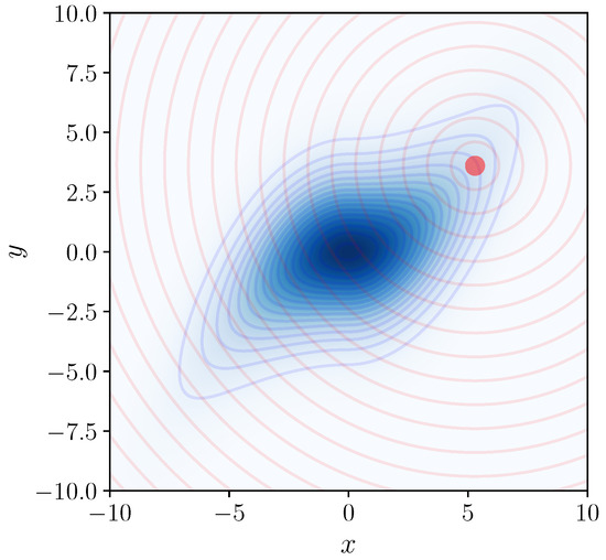
Figure 1. To evaluate the log-probability (or density) of the blue probability distribution near the red point, Nested Sampling can be used, with the blue distribution playing the role of the “prior” in NS, and the Euclidean distance from the red point (illustrated with red contours) playing the role of the negative log-likelihood. Averaging over selections of the red point gives an estimate of the entropy of the blue distribution.

If we actually want the differential entropy

$$\begin{array}{cc}\hfill H\left(\mathit{\theta }\right)& =-\int p(\mathit{\theta })logp(\mathit{\theta })d\mathit{\theta },\hfill \end{array}$$

(27)

we can use the fact that density equals mass divided by volume. Assume r is small, so that

$$\begin{array}{cc}\hfill P(d(\mathit{\theta };{\mathit{\theta }}_{\mathrm{ref}})<r|{\mathit{\theta }}_{\mathrm{ref}})& \approx p\left({\mathit{\theta }}_{\mathrm{ref}}\right){\int }_{d(\mathit{\theta };{\mathit{\theta }}_{\mathrm{ref}})<r}d\mathit{\theta }\hfill \end{array}$$

(28)

$$\begin{array}{c}=p\left({\mathit{\theta }}_{\mathrm{ref}}\right)V,\hfill \end{array}$$

(29)

where V is the volume of the region where $d(\mathit{\theta };{\mathit{\theta }}_{\mathrm{ref}})<r$. Then, $H\left(\mathit{\theta }\right)={⟨\left(\mathrm{depth}\right)⟩}_{p\left(\mathit{\theta }\right)}+logV\left(r\right)$. It is important to remember that the definition of volume here is in terms of the coordinates $\mathit{\theta }$, and that a change of coordinates (or a change of the definition of the distance function) would result in a different value of the differential entropy. This is equivalent to counting possibilities or volumes with a different choice of base measure $q\left(\mathit{\theta }\right)$.

Reducing r towards zero ought to lead to a more accurate result because the probability density at a point will be more accurately approximated by the probability of a small region containing the point, divided by the volume of that region. On the other hand, smaller values of r will lead to more Nested Sampling iterations required, and hence less accuracy in the depth estimates. Thus, there is a an awkward trade-off involved in choosing the value of r, which will need to be investigated more thoroughly in the future. However, the algorithm as it currently stands ought to be useful for calculating the entropies of any low-to-moderate dimensional functions of an underlying high-dimensional space.

If the distance function $d({\mathit{\theta }}_{\mathrm{ref}},\mathit{\theta })$ is chosen to be Euclidean, the constraint $d({\mathit{\theta }}_{\mathrm{ref}},\mathit{\theta })<r$ corresponds to a ball in the space of possible ${\mathit{\theta }}_{\mathrm{ref}}$ values. The volume of such a ball, of radius r in n dimensions, is

$$\begin{array}{cc}\hfill V& =\frac{{\left(\pi r^2\right)}^{n/2}}{\left(\frac{n}{2}\right)!}.\hfill \end{array}$$

(30)

In one dimension, if the threshold r is not small, we might think we are calculating the entropy associated with the question ‘what is $\mathit{\theta }$, to within a tolerance of $\pm r$?’. This is not quite correct. See Appendix A for a discussion of this type of question.

In the following sections, I demonstrate the algorithm on three example problems. For each of the examples, I used 1000 repetitions of NS (i.e., 1000 reference particles), and used 10 NS particles and 10,000 MCMC steps per NS iteration.

5. Example 1: Entropy of a Prior for the Data

This example demonstrates how the algorithm may be used to determine the entropy for a quantity whose distribution can only be sampled, in this case, a prior distribution over datasets.

Consider the basic statistics problem of inferring a quantity $\mu$ from 100 observations $\mathit{x}=\{x_1,\dots ,x_{100}\}$ whose probability distribution (conditional on $\mu$) is

$$\begin{array}{cc}\hfill p\left(x_i\right|\mu )& \sim \mathrm{Normal}(\mu ,1).\hfill \end{array}$$

(31)

I assumed a Normal$(0,{10}^2)$ prior for $\mu$. Before getting the data, the prior information is described by the joint distribution

$$\begin{array}{cc}\hfill p(\mu ,\mathit{x})& =p\left(\mu \right)p\left(\mathit{x}\right|\mu ).\hfill \end{array}$$

(32)

The prior over datasets is given by the marginal distribution

$$\begin{array}{cc}\hfill p(\mathit{x})& =\int p(\mu ,\mathit{x})d\mu .\hfill \end{array}$$

(33)

This is the distribution whose differential entropy I seek in this section. Its true value is available analytically in this case, by noting that the posterior is available in closed form for any dataset:

$$\begin{array}{cc}\hfill \mu |\mathit{x}& \sim \mathrm{Normal}\left(\frac{1}{100.01}\sum _{i=1}^{100}{x}_i,{\left[\frac{10}{\sqrt{10001}}\right]}^2\right),\hfill \end{array}$$

(34)

which enables the calculation of the mutual information and hence $H\left(\mathit{x}\right)$. The true value of $H\left(\mathit{x}\right)$ is $146.499$ nats. However, in most situations, the entropy of a marginal distribution such as this is not available in closed form.

To use the algorithm, a distance function $d(;)$ must be defined, to quantify how far the NS particles are from the reference particle. To calculate the entropy of the data, I applied the algorithm in the joint space of possible parameters and datasets, i.e., distribution of reference particles followed Equation 32. For the distance function, which helps the NS particles approach the reference particle, I used a simple Euclidean metric in the space of datasets:

$$\begin{array}{cc}\hfill d\left(\mathit{\theta };{\mathit{\theta }}_{\mathrm{ref}}\right)& =\sqrt{\sum _{i=1}^{100}{\left(x_i-x_{\mathrm{ref},i}\right)}^2}.\hfill \end{array}$$

(35)

Since the distance function refers only to the data $\mathit{x}$ and not the parameter $\mu$, the sampling is effectively done in the space of possible datasets only — the parameter $\mu$ can be thought of as merely a latent variable allowing $p\left(\mathit{x}\right)$ to be explored conveniently.

I ran the algorithm and computed the average depth using a tolerance of $r={10}^{-3}\sqrt{100}$, so that the root mean square difference between points in the two datasets was about ${10}^{-3}$. From the algorithm, the estimate of the expected depth was

$$\begin{array}{cc}\hfill ⟨{\left(\mathrm{depth}\right)}_{\mathit{x}}⟩& =698.25\pm 0.34.\hfill \end{array}$$

(36)

The uncertainty here is the standard error of the mean, i.e., the standard deviation of the depth estimates divided by square root of the number of NS repetitions (the number of reference particles whose depth was evaluated).

The log-volume of a 100-dimensional ball of radius $r={10}^{-3}\sqrt{100}$ is $-551.76$. Therefore, the differential entropy is estimated to be

$$\begin{array}{cc}\hfill H\left(\mathit{x}\right)& \approx 146.49\pm 0.34,\hfill \end{array}$$

(37)

which is very close to the true value (perhaps suspiciously close, but this was just a fluke).

To carry out the sampling for this problem, Metropolis–Hastings moves that explore the joint prior distribution $p(\mu ,\mathit{x})$ had to be implemented. Four basic kinds of proposals were used: (i) those which change $\mu$ while leaving $\mathit{x}$ fixed; (ii) those which change $\mu$ and shift $\mathit{x}$ correspondingly; (iii) those which resample a subset of the xs from $p\left(\mathit{x}\right|\mu )$; and (iv) those which move a single x slightly.

6. Example 2: Measuring the Period of an Oscillating Signal

In physics and astronomy, it is common to measure an oscillating signal at a set of times $\{t_1,\dots ,t_n\}$, in order to infer the amplitude, period, and phase of the signal. Here, I demonstrate the algorithm on a toy version of Bayesian experimental design: at what times should the signal be observed in order to obtain as much information as possible about the period? To answer this, we need to be able to calculate the mutual information between the unknown period and the data.

As the algorithm lets us calculate the entropy of any distribution that can be sampled by MCMC, there are several options. The mutual information can be written in various ways, such as the following:

$$\begin{array}{cc}\hfill I(\mathit{\theta };\mathit{d})& =H\left(\mathit{\theta }\right)+H\left(\mathit{d}\right)-H(\mathit{\theta },\mathit{d}),\hfill \end{array}$$

(38)

$$\begin{array}{cc}\hfill I(\mathit{\theta };\mathit{d})& =H\left(\mathit{d}\right)-H\left(\mathit{d}\right|\mathit{\theta }),\hfill \end{array}$$

(39)

$$\begin{array}{cc}\hfill I(\mathit{\theta };\mathit{d})& =H\left(\mathit{\theta }\right)-H\left(\mathit{\theta }\right|\mathit{d}),\hfill \end{array}$$

(40)

$$\begin{array}{cc}\hfill I(\mathit{\theta };\mathit{d})& =\int p\left(\mathit{d}\right)D_{\mathrm{KL}}\left(p\left(\mathit{\theta }\right|\mathit{d}\left)\right|\left|p\right(\mathit{\theta })\right)d\mathit{d},\hfill \end{array}$$

(41)

$$\begin{array}{cc}\hfill I(\mathit{\theta };\mathit{d})& =D_{\mathrm{KL}}\left(p(\mathit{\theta },\mathit{d})\left|\right|p\left(\mathit{\theta }\right)p\left(\mathit{d}\right)\right).\hfill \end{array}$$

(42)

In a Bayesian problem where $\mathit{\theta }$ is an unknown parameter and $\mathit{d}$ is data, the first and second formulas would be costly to compute because the high dimensional probability distribution for the dataset would require a large number of NS iterations to compute $H\left(\mathit{d}\right)$ and $H(\mathit{\theta },\mathit{d})$. The fourth involves the Kullback–Leibler divergence from the prior to the posterior, averaged over all possible datasets. This is straightforward to approximate with standard Nested Sampling, but the estimate for a given dataset may be biased. It is quite plausible that the bias is negligible compared to the variance from averaging over many datasets. This is probably true in many situations.

However, more significantly, the above method would not work if we want $I(\mathit{\theta };\mathit{d})$ for a single parameter or a subset of them, rather than for all of the parameters. The prior-to-posterior KL divergence measured by standard NS is the amount learned about all parameters, including nuisance parameters. Therefore, I adopted the third formula as the best way to compute $I(\mathit{\theta };\mathit{d})$. In the sinusoidal example, the parameter of interest is the period, whereas the model will contain other parameters as well. Since the period will have its prior specified explicitly, $H\left(\mathit{\theta }\right)$ will be available analytically. I then use the algorithm to obtain $H\left(\mathit{\theta }\right|\mathit{d})$ as follows:

$$\begin{array}{cc}\hfill H\left(\mathit{\theta }\right|\mathit{d})& =\int p\left({\mathit{d}}_{\mathrm{ref}}\right)H\left(\mathit{\theta }\right|\mathit{d}={\mathit{d}}_{\mathrm{ref}})d{\mathit{d}}_{\mathrm{ref}}.\hfill \end{array}$$

(43)

This is an expected value over datasets, of the entropy of the posterior given each dataset. I ran the algorithm by generating reference particles from $p(\mathit{\theta },\mathit{d})$, i.e., generating parameter values from the prior, along with corresponding simulated datasets. Given each simulated dataset, I used NS to compute an unbiased estimate of $H\left(\mathit{\theta }\right|\mathit{d}={\mathit{d}}_{\mathrm{ref}})$, by evolving a set of particles (initially from the posterior) towards the reference particle. The role of the “prior” in the NS is actually taken by the posterior, and the “likelihood” was minus a distance function defined in terms of the parameter(s) of interest.

To generate the initial NS particles from the posterior, I used standard MCMC (targeting the posterior), initialised at the $\mathit{\theta }$-value that produced the simulated dataset ${\mathit{d}}_{\mathrm{ref}}$, which is a perfect sample from the posterior.

6.1. Assumptions

I consider two possible observing strategies, both involving $n=101$ measurements. The ‘even’ strategy has observations at times

$$\begin{array}{c}\hfill t_i=\frac{i-1}{n-1}\end{array}$$

(44)

for $i\in \{1,2,\dots ,101\}$; that is, the observation times are $0,0.01,0.02,\dots ,0.99,1$—evenly spaced from $t=0$ to $t=1$, including the endpoints. The second, ‘uneven’ observing strategy schedules the observations according to

$$\begin{array}{c}\hfill t_i={\left(\frac{i-\frac{1}{2}}{n}\right)}^3,\end{array}$$

(45)

which schedules observations close together initially, and further apart as time goes on.

A purely sinusoidal signal has the form

$$\begin{array}{cc}\hfill y\left(t\right)& =Asin\left(\frac{2\pi t}{T}+\varphi \right),\hfill \end{array}$$

(46)

where A is the amplitude, T is the period, and $\varphi$ is the phase. Throughout this section, I parameterise the period by its logarithm, $\tau ={log}_{10}T$. I assumed the following priors:

$$\begin{array}{cc}\hfill lnA& \sim \mathrm{Normal}\left(0,{0.1}^2\right),\hfill \end{array}$$

(47)

$$\begin{array}{cc}\hfill \tau & \sim \mathrm{Uniform}(-1,0),\hfill \end{array}$$

(48)

$$\begin{array}{cc}\hfill \varphi & \sim \mathrm{Uniform}(0,2\pi ),\hfill \end{array}$$

(49)

and the following conditional prior for the data:

$$\begin{array}{cc}\hfill Y_i|A,T,\varphi & \sim \mathrm{Normal}\left(y\left(t_i\right),{0.1}^2\right).\hfill \end{array}$$

(50)

That is, the data is just the signal $y\left(t\right)$ observed at particular times $\{t_1,\dots ,t_n\}$, with Gaussian noise of standard deviation 0.1. The amplitude of the sinusoid is very likely to be around 10 times the noise level, and the period is between 0.1 times and 1 time the duration of the data. An example signal observed with the even and uneven observing schedules is shown in Figure 2.

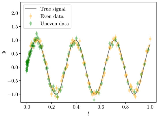
Figure 2. A signal with true parameters $A=1$, $\tau =-0.5$, and $\varphi =0$, observed with noise standard deviation 0.1 with the even (gold points) and uneven (green points) observing strategies.

To carry out the sampling for this problem, Metropolis–Hastings moves that explore the posterior distribution $p(A,\tau ,\varphi |\mathit{Y})$ had to be implemented. I used heavy-tailed proposals (as in Section 8.3 of Brewer and Foreman-Mackey [23]), which modified one parameter at a time.

6.2. Results

Letting $\tau ={log}_{10}T$, and treating A and $\varphi$ are nuisance parameters, I calculated the conditional entropy $H\left(\tau \right|\mathit{Y})$ using the algorithm with a tolerance of $r={10}^{-5}$. The distance function was just the absolute difference between $\tau$ and ${\tau }_{\mathrm{ref}}$.

The result was

$$\begin{array}{cc}\hfill ⟨\left(\mathrm{depth}\right)⟩& =5.379\pm 0.038.\hfill \end{array}$$

(51)

Converting to a differential entropy by adding $ln\left(2r\right)=-10.820$, the conditional entropy is

$$\begin{array}{cc}\hfill H\left(\tau \right|\mathit{Y})& =-5.441\pm 0.038\mathrm{nats}.\hfill \end{array}$$

(52)

Since the Uniform(0,1) prior for $\tau$ has a differential entropy of zero, the mutual information is $I(\tau ;\mathit{Y})=H\left(\tau \right)-H\left(\tau \right|\mathit{Y})=5.441\pm 0.038$ nats.

The results for the uneven observing schedule were

$$\begin{array}{cc}\hfill ⟨\left(\mathrm{depth}\right)⟩& =5.422\pm 0.038,\hfill \end{array}$$

(53)

$$\begin{array}{cc}\hfill H\left(\tau \right|\mathit{Y})& =-5.398\pm 0.038,\hfill \end{array}$$

(54)

$$\begin{array}{cc}\hfill I(\tau ;\mathit{Y})& =5.398\pm 0.038.\mathrm{nats}.\hfill \end{array}$$

(55)

The difference in mutual information between the two observation schedules is trivial. The situation may be different if we had allowed for shorter periods to be possible, as irregular observing schedules are known to reduce aliasing and ambiguity in the inferred period [24]. When inferring the period of an oscillating signal, multimodal posterior distributions for the period are common [17,25]. The multimodality of the posterior here raises an interesting issue. Is the question we really want answered “what is the value of T precisely?”, to which the mutual information relates? Most practicing scientists would not feel particularly informed to learn that the vast majority of possibilities had been ruled out, if the posterior still consisted of several widely separated modes! Perhaps, in some applications, a more appropriate question is “what is the value of T to within ± 10%”, or something along these lines. See Appendix A for more about this issue.

In a serious experimental design situation, the relevance is not the only consideration (or the answer to every experimental design problem would be to obtain more data without limit), but it is a very important one.

7. Example 3: Data with Pareto Distribution

Consider a situation where the probability distribution for some data values $\mathit{x}=\{x_1,x_2,\dots ,x_n\}$ is a Pareto distribution, conditional on a minimum value $x_{\min }=1$ and a slope $\alpha$:

$$\begin{array}{cc}\hfill p\left(\mathit{x}\right|\alpha )& =\prod _{i=1}^n\frac{\alpha }{x_i^{\alpha +1}},\hfill \end{array}$$

(56)

where all of the $x_i$ are greater than $x_{\min }=1$. If $\alpha$ is relatively low (close to zero), then this distribution is very heavy-tailed, and as $\alpha$ increases, the probability density for the xs concentrates just above $x=1$.

With heavy-tailed distributions, it can be difficult to predict future observations from past ones, a notion popularised by Taleb [26]. This occurs for three main reasons. First, the observations may not provide much information about the parameters (in this case, $\alpha$). Second, even conditional on the parameters, the predictive distribution for future data can be heavy-tailed, implying a lot of uncertainty. Finally, one may always doubt the probability assignment on which such a calculation is based. However, the data clearly provides some nonzero amount of information about the future.

Consider $n=100$ data values, partitioned into two halves, so $\mathit{Y}=\{x_1,\dots ,x_{50}\}=\{y_1,\dots ,y_{50}\}$ is the first half of the data and $\mathbf{z}=\{x_{51},\dots ,x_{100}\}=\{z_1,\dots ,z_{50}\}$ is the second half. Let $y_{\mathrm{tot}}$ and $z_{\mathrm{tot}}$ be the totals of the two subsets of the data:

$$\begin{array}{cc}\hfill y_{\mathrm{tot}}& =\sum _{i=1}^{50}{y}_i,\hfill \end{array}$$

(57)

$$\begin{array}{cc}\hfill z_{\mathrm{tot}}& =\sum _{i=1}^{50}{z}_i.\hfill \end{array}$$

(58)

In this section, I use the algorithm to answer the questions: (i) How uncertain is $y_{\mathrm{tot}}$?; (ii) How uncertain is $z_{\mathrm{tot}}$?; and (iii) How informative is $y_{\mathrm{tot}}$ about $z_{\mathrm{tot}}$? These are quantified by $H\left(y_{\mathrm{tot}}\right)$, $H\left(z_{\mathrm{tot}}\right)$, and $I(y_{\mathrm{tot}};z_{\mathrm{tot}}),$ respectively. This can be done despite the fact that $\alpha$ is unknown.

The prior for $\alpha$ was chosen to be lognormal such that the prior median of $\alpha$ is 1 and the prior standard deviation of $ln\alpha$ is also 1. Due to the heavy-tailed nature of the Pareto distribution, I ran the algorithm in terms of $ln{y}_{\mathrm{tot}}$ and $ln{z}_{\mathrm{tot}}$. This affects the differential entropies but not the mutual information (which is invariant under changes of parameterisation). The joint distribution for $ln{y}_{\mathrm{tot}}$ and $ln{z}_{\mathrm{tot}}$, whose properties I aimed to obtain, is shown in Figure 3.

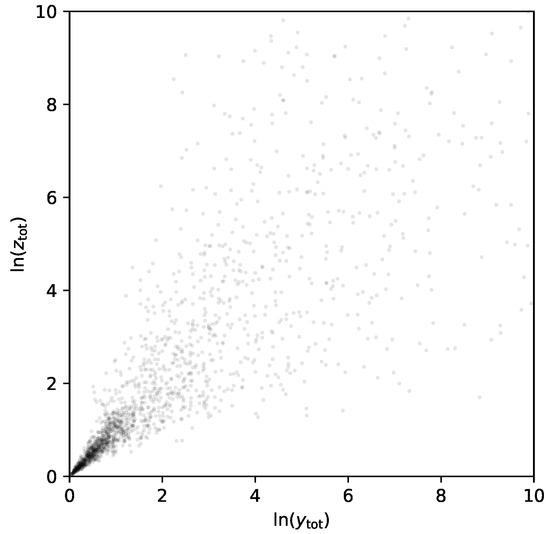
Figure 3. The joint distribution for the log-sum of the first half of the ‘Pareto data’ and the second half. The goal is to calculate the entropy of the marginal distributions, the entropy of the joint distribution, and hence the mutual information. The distribution is quite heavy tailed despite the logarithms, and extends beyond the domain shown in this plot.

Three types of Metropolis–Hastings proposals were used for this example: (i) a proposal that changes $\alpha$ and modifies all of the xs accordingly; (ii) a proposal that resamples a subset of the xs from the Pareto distribution; and (iii) a proposal that moves a single x-value slightly. A fourth proposal that moves $\alpha$ while keeping $\mathit{x}$ fixed, i.e., a posterior-sampling move, was not implemented.

To compute the entropy of $ln{y}_{\mathrm{tot}}$, the distance function was just the absolute value of the distance between the NS particles and the reference particle in terms of $ln{y}_{\mathrm{tot}}$. The result, using a tolerance of $r={10}^{-3}$, was:

$$\begin{array}{cc}\hfill ⟨{\left(\mathrm{depth}\right)}_{ln{y}_{\mathrm{tot}}}⟩& =8.851\pm 0.057.\hfill \end{array}$$

(59)

Correcting for the volume factor yields a differential entropy estimate of $H(ln{y}_{\mathrm{tot}})=2.366\pm 0.057$ nats. By the symmetry of the problem specification, $H(ln{z}_{\mathrm{tot}})=H(ln{y}_{\mathrm{tot}})$.

The joint entropy $H(ln{y}_{\mathrm{tot}},ln{z}_{\mathrm{tot}})$ was also estimated by using a Euclidean distance function and a tolerance of ${10}^{-3}$. The result was

$$\begin{array}{cc}\hfill ⟨{\left(\mathrm{depth}\right)}_{(ln{y}_{\mathrm{tot}},ln{z}_{\mathrm{tot}})}⟩& =16.03\pm 0.11.\hfill \end{array}$$

(60)

Applying the log-volume correction yields a differential entropy estimate of $H(ln{y}_{\mathrm{tot}},ln{z}_{\mathrm{tot}})=3.40\pm 0.11$ nats. Therefore, the mutual information is

$$\begin{array}{cc}\hfill I(y_{\mathrm{tot}};z_{\mathrm{tot}})& =H(ln{y}_{\mathrm{tot}})+H(ln{z}_{\mathrm{tot}})-H(ln{y}_{\mathrm{tot}},ln{z}_{\mathrm{tot}})\hfill \end{array}$$

(61)

$$\begin{array}{c}=1.130\pm 0.082\mathrm{nats}.\hfill \end{array}$$

(62)

The variance of this mutual information estimate was reduced by using a common sequence of reference points for the marginal and joint entropy runs. This is an instance of the ‘common random numbers’ technique (http://demonstrations.wolfram.com/TheMethodOfCommonRandomNumbersAnExample/). In short, for those reference particles with a large depth in terms of the $ln{y}_{\mathrm{tot}}$ distance function, the depth in terms of the $(ln{y}_{\mathrm{tot}},ln{z}_{\mathrm{tot}})$ distance function was also large. Since the mutual information involves a difference of the averages of these depths, it is more accurate to compute the average difference (i.e., compute the two depths using the same reference particle, to compute the difference between the two depths) than the difference of the averages.

8. Computational Cost and Limitations

The computational resources needed to compute these quantities was quite large, as Nested Sampling appears in the inner loop of the algorithm. However, it is worth reflecting on the complexity of the calculation that has been done.

In a Bayesian inference problem with parameters $\mathit{\theta }$ and data $\mathit{d}$, the mutual information is

$$\begin{array}{cc}\hfill I(\mathit{\theta };\mathit{d})& =\int \int p(\mathit{\theta },\mathit{d})ln\left[\frac{p(\mathit{\theta },\mathit{d})}{p\left(\mathit{\theta }\right)p\left(\mathit{d}\right)}\right]d\mathit{\theta }d\mathit{d},\hfill \end{array}$$

(63)

and this measures the dependence between $\mathit{\theta }$ and $\mathit{d}$. A Monte Carlo strategy to evaluate this is to sample from $p(\mathit{\theta },\mathit{d})$ and average the value of the logarithm, which involves computing the log-evidence

$$\begin{array}{c}\hfill lnp\left(\mathit{d}\right)=ln\left[\int p(\mathit{\theta })p(\mathit{d}|\mathit{\theta })d\mathit{\theta }\right]\end{array}$$

(64)

for each possible data set. Computing $p\left(\mathit{d}\right)$ for even a single data set has historically been considered difficult.

However, if we want the mutual information between the data and a subset of the parameters (i.e., there are nuisance parameters we do not care about), things become even more tricky. Suppose we partition the parameters $\mathit{\theta }$ into important parameters $\mathit{\varphi }$ and nuisance parameters $\mathit{\eta }$, such that we want to calculate the mutual information $I(\mathit{\varphi };\mathit{d})$. This is given by

$$\begin{array}{cc}\hfill I(\mathit{\varphi };\mathit{d})& =\int \int p(\mathit{\varphi },\mathit{d})ln\left[\frac{p(\mathit{\varphi },\mathit{d})}{p\left(\mathit{\varphi }\right)p\left(\mathit{d}\right)}\right]d\mathit{\varphi }d\mathit{d},\hfill \end{array}$$

(65)

which is equivalent to Equation 63 but with $\mathit{\theta }$ replaced throughout by $\mathit{\varphi }$. However, this is an even more difficult calculation than before, as $p\left(\mathit{d}\right|\mathit{\varphi })$, the marginal likelihood function with the nuisance parameters integrated out, is typically unavailable in closed form. If we were to marginalise out the nuisance parameters $\mathit{\eta }$ explicitly, this would give us Equation 65 with every probability distribution written as an explicit integral over $\mathit{\eta }$:

$$\begin{array}{cc}\hfill I(\mathit{\varphi };\mathit{d})& =\int \int \left(\int p(\mathit{\varphi },\mathit{\eta })p(\mathit{d}|\mathit{\varphi },\mathit{\eta })d\mathit{\eta }\right)ln\left[\frac{\int p(\mathit{\varphi },\mathit{\eta })p\left(\mathit{d}\right|\mathit{\varphi },\mathit{\eta })d\mathit{\eta }}{p\left(\mathit{\varphi }\right)\int p(\mathit{\varphi },\mathit{\eta })p\left(\mathit{d}\right|\mathit{\varphi },\mathit{\eta })d\mathit{\varphi }\mathit{d}\mathit{\eta }}\right]d\mathit{\varphi }d\mathit{d}.\hfill \end{array}$$

(66)

It should not be surprising that this is costly. Indeed, it seems possible to me that any general algorithm for computing entropies will have the property that NS (or a similar algorithm capable of measuring small volumes) appears in an inner loop, since entropies are sums of terms, each of which relates to the downset of a given statement—the downset of a statement S being the set of all statements that imply S [3].

The current implementation of the algorithm (see Appendix B) is in C++ and has not been parallelised. Given the high computational costs, parallelisation should be attempted. This could follow the method of [21], or alternatively, different threads could work on different reference particles simultaneously.

The algorithm as presented will tend to become less accurate on high dimensional problems, as the required depth of the runs will increase correspondingly, since many NS iterations will be required to get a high dimensional vector of quantities to be close to the reference vector. The accuracy of the $ln\left(\mathrm{depth}\right)$ estimates should degrade in proportion to $\sqrt{\left(\mathrm{depth}\right)}$, due to the Poisson-process nature of the $-lnX$ sequence.

Throughout this paper, the question of how to sample from the constrained distributions required by NS has not been discussed in detail. For the examples, I used the original Skilling [11] suggestion of using a short MCMC run initialised at a surviving point. In some problems, this will not be effective, and this will cause the resulting estimates to be incorrect, as in standard Nested Sampling applications. Testing the sensitivity of the results to changes in the number of MCMC steps used is a simple way to increase one’s confidence in the results, but is not a guarantee (no general guarantee can exist, because any algorithm based on sampling a subset of a space might miss a crucial but hard-to-locate dominant spike). Despite this weakness, I hope the algorithm will be useful in a wide range of applications.

References

- Shannon, C.E. A mathematical theory of communication. Bell Syst. Tech. J. 1948, 27, 379–423. [Google Scholar] [CrossRef]
- Cover, T.M.; Thomas, J.A. Elements of Information Theory; Wiley & Sons: Hoboken, NJ, USA, 2012. [Google Scholar]
- Knuth, K.H. Toward question-asking machines: The logic of questions and the inquiry calculus. In Proceedings of the 10th International Workshop On Artificial Intelligence and Statistics, Barbados, 6–8 January 2005. [Google Scholar]
- Knuth, K.H.; Skilling, J. Foundations of inference. Axioms 2012, 1, 38–73. [Google Scholar] [CrossRef]
- Caticha, A.; Giffin, A. Updating probabilities. AIP Conf. Proc. 2006, 31. [Google Scholar] [CrossRef]
- Szabó, Z. Information theoretical estimators toolbox. J. Mach. Learn. Res. 2014, 15, 283–287. [Google Scholar]
- Jaynes, E.T. Probability theory: The logic of science; Cambridge university press: New York, NY, USA, 2003. [Google Scholar]
- MacKay, D.J. Information Theory, Inference and Learning Algorithms; Cambridge university press: New York, NY, USA, 2003. [Google Scholar]
- Caticha, A. Lectures on probability, entropy, and statistical physics. arXiv 2008, arXiv:0808.0012. [Google Scholar]
- Bernardo, J.M. Reference analysis. Handb. Stat. 2005, 25, 17–90. [Google Scholar]
- Skilling, J. Nested sampling for general Bayesian computation. Bayesian anal. 2006, 1, 833–859. [Google Scholar] [CrossRef]
- Feroz, F.; Hobson, M.; Bridges, M. MultiNest: An efficient and robust Bayesian inference tool for cosmology and particle physics. Mon. Not. R. Astron. Soc. 2009, 398, 1601–1614. [Google Scholar] [CrossRef]
- Brewer, B.J.; Pártay, L.B.; Csányi, G. Diffusive nested sampling. Stat. Comput. 2011, 21, 649–656. [Google Scholar] [CrossRef]
- Handley, W.; Hobson, M.; Lasenby, A. PolyChord: Next-generation nested sampling. Mon. Not. R. Astron. Soc. 2015, 453, 4384–4398. [Google Scholar] [CrossRef]
- Knuth, K.H.; Habeck, M.; Malakar, N.K.; Mubeen, A.M.; Placek, B. Bayesian evidence and model selection. Digit. Signal Process. 2015, 47, 50–67. [Google Scholar] [CrossRef]
- Pullen, N.; Morris, R.J. Bayesian model comparison and parameter inference in systems biology using nested sampling. PLoS ONE 2014, 9, e88419. [Google Scholar] [CrossRef] [PubMed]
- Brewer, B.J.; Donovan, C.P. Fast Bayesian inference for exoplanet discovery in radial velocity data. Mon. Not. R. Astron. Soc. 2015, 448, 3206–3214. [Google Scholar] [CrossRef]
- Pártay, L.B.; Bartók, A.P.; Csányi, G. Efficient sampling of atomic configurational spaces. J. Phys. Chem. B 2010, 114, 10502–10512. [Google Scholar] [CrossRef] [PubMed]
- Baldock, R.J.; Pártay, L.B.; Bartók, A.P.; Payne, M.C.; Csányi, G. Determining pressure-temperature phase diagrams of materials. Phys. Rev. B 2016, 93, 174108. [Google Scholar] [CrossRef]
- Martiniani, S.; Stevenson, J.D.; Wales, D.J.; Frenkel, D. Superposition enhanced nested sampling. Phys. Rev. X 2014, 4, 031034. [Google Scholar] [CrossRef]
- Henderson, R.W.; Goggans, P.M.; Cao, L. Combined-chain nested sampling for efficient Bayesian model comparison. Digit. Signal Process. 2017, 70, 84–93. [Google Scholar] [CrossRef]
- Walter, C. Point process-based Monte Carlo estimation. Stat. Comput. 2017, 27, 219–236. [Google Scholar] [CrossRef]
- Brewer, B.J.; Foreman-Mackey, D. DNest4: Diffusive Nested Sampling in C++ and Python. J. Stat. Softw. 2016, in press. [Google Scholar]
- Bretthorst, G.L. Nonuniform sampling: Bandwidth and aliasing. AIP Conf. Proc. 2001, 567. [Google Scholar] [CrossRef]
- Gregory, P.C. A Bayesian Analysis of Extrasolar Planet Data for HD 73526. Astrophys. J. 2005, 631, 1198–1214. [Google Scholar] [CrossRef]
- Taleb, N.N. The Black Swan: The Impact of the Highly Improbable; Random House: New York, NY, USA, 2007. [Google Scholar]
© 2017 by the author. Licensee MDPI, Basel, Switzerland. This article is an open access article distributed under the terms and conditions of the Creative Commons Attribution (CC BY) license (http://creativecommons.org/licenses/by/4.0/).