Abstract
Information geometry enables a deeper understanding of the methods of statistical inference. In this paper, the problem of nonlinear parameter estimation is considered from a geometric viewpoint using a natural gradient descent on statistical manifolds. It is demonstrated that the nonlinear estimation for curved exponential families can be simply viewed as a deterministic optimization problem with respect to the structure of a statistical manifold. In this way, information geometry offers an elegant geometric interpretation for the solution to the estimator, as well as the convergence of the gradient-based methods. The theory is illustrated via the analysis of a distributed mote network localization problem where the Radio Interferometric Positioning System (RIPS) measurements are used for free mote location estimation. The analysis results demonstrate the advanced computational philosophy of the presented methodology.
1. Introduction
Information geometry, pioneered by Rao in the 1940s [1] and further developed by Chentsov [2], Efron [3,4] and Amari [5,6], considers the statistical relationships between families of probability densities in terms of the geometric properties of Riemann manifolds. It is the study of intrinsic properties of manifolds of probability distributions [7], where the ability of the data to discriminate those distributions is translated into a Riemannian metric. Specifically, the Fisher information gives a local measure of discrimination of the distributions which immediately provides a Riemannian metric on the parameter manifold of the distributions [1]. In particular, the collection of probability density functions called curved exponential families, which encapsulate important distributions in many real world problems, have been treated using this framework [5].
The main tenet of information geometry is that many important notions in probability theory, information theory and statistics can be treated as structures in differential geometry by regarding a space of probabilities as a differentiable manifold endowed with a Riemannian metric and a family of affine connections, including but not exclusively, the canonical Levi-Civita affine connection [6]. By providing a means to analyse the Riemannian geometric properties of various families of probability density functions, information geometry offers comprehensive results about statistical problems simply by considering them as geometrical objects. Information geometry opens new prospect to study the intrinsic geometrical nature of information theory and provides a new way to deal with statistical problems on manifolds. For example, Smith [8] studied the intrinsic Cramér-Rao bounds on estimation accuracy for the estimation problems on arbitrary manifolds where the set of intrinsic coordinates is not apparent, and derived the intrinsic bounds in the examples of covariance matrix and subspace estimation. Srivastava et al. [9,10] addressed the geometric subspace estimation and target tracking problems under a Bayesian framework. Bhattacharya and Patrangenaru [11] treated the general problem of estimation on Riemannian manifolds.
As this new general theory reveals the capability of defining a new perspective on existing questions, many researchers are extending their work on this geometric theory of information to new areas of application and interpretation. For example, a most important milestone in the area of signal processing is the work of Richardson where the geometric perspective clearly indicates the relationship between turbo-decoding and maximum-likelihood decoding [12]. The results of Amari et al. on the information geometry of turbo and low-density parity-check codes extend the geometrical framework initiated by Richardson to the information geometrical framework of dual affine connections [13]. Other investigations include the geometrical interpretation of fading in wireless networks [14]; the geometrical interpretation of the solution to the multiple hypothesis testing problem in the asymptotic limit developed by Westover [15]; and a geometric characterization of multiuser detection for synchronous DS/CDMA channels [16]. Recently, the framework of information geometry has been applied to address issues in the application of sensor networks such as target resolvability [17], radar information resolution [18] and passive sensor scheduling [19,20].
In this paper, we mainly focus on the nonlinear estimation problem and illustrate how it can benefit from the powerful methodologies of information geometry. The geometric interpretation for the solution to the maximum likelihood estimation for curved exponential families and the convergence of the gradient-based methods (such as Newton’s method and the Fisher scoring algorithm) are demonstrated via the framework developed by Efron and Amari et al. Our essential motivation of this work is to provide some insights into the nonlinear parameter estimation problems in signal processing using the theory of information geometry. By gaining a better understanding of the existing algorithms through the use of information geometric method, we are, hopefully, enabled to derive better algorithms for solving non-linear problems.
The work described in this paper consists of the following aspects. Firstly, an iterative maximum likelihood estimator (MLE) for estimating non-random parameters with measurement of the curved exponential distributions is presented. The estimator belongs to the gradient-based methods that operate on statistical manifolds and can be seen as a generalization of Newton’s method to families of probability density functions and their relevant statistics. Its interpretation in terms of differential and information geometry provides insight into its optimality and convergence. Then, by utilizing the properties of exponential families and thus identifying the parameters on statistical manifolds, the implementation of the presented MLE algorithm is simplified via reparametrization. Furthermore, it is shown that the associated stochastic estimation problem reduces to a deterministic optimization problem with respect to the measures (statistics) defined over the distributions. Finally, an example of a one-dimensional curved Gaussian is presented to demonstrate the method in the manifold. A practical example of distributed mote network localization using the Radio Interferometric Positioning System (RIPS) measurements is given to demonstrate the issues addressed in this paper. The performance of the estimator is discussed.
In the next section, classical nonlinear estimation via natural gradient MLE for curved exponential families is derived. The reparametrization from local parameters to natural parameters and expectation parameters is highlighted. In Section 3, the principles of information geometry are introduced. Further, the geometric interpretation for the presented iterative maximum likelihood estimator and the convergence of the developed algorithm is demonstrated via the properties of statistical manifolds. In Section 4, a one parameter estimation example is presented to illustrate the geometric operation of the algorithm. The performance and efficiency of the algorithm are further demonstrated via a mote localization example using RIPS measurements. Finally, conclusions are made in Section 5.
2. Nonlinear Estimation via Natural Gradient MLE
In probability and statistics, exponential families (including the normal, exponential, Gamma, Chi-squared, Beta, Poisson, Bernoulli, multinomial and many others) are an important class of distributions naturally considered. There is a framework for selecting a possible alternative parameterization of these distributions, in terms of the natural parameters, and for defining useful statistics, called the natural statistics of the families. When the natural parameters in exponential families are nonlinear functions of some “local” parameters, the distributions involved are in the curved exponential families. While curved exponential families which encapsulate important distributions are more suitable to describe many real world problems, the estimation of local parameters is often non-trivial because of the nonlinearity in parameters.
In this section, a natural gradient based maximum likelihood estimator is derived to address a nonlinear estimation problem for curved exponential families. Although the estimator has been well-known as the Fisher scoring method in the literature, the interpretation of its iterative operations via the theory of information geometry is interesting and will be presented in the following section.
The general form of a curved exponential family [5] can be expressed as
where is a vector valued measurement, are the natural coordinates or canonical parameters, denote local parameters and are sufficient statistics for , and functions on the measurement space with elements denoted by . The function is called the potential function of the exponential family and it is found from the normalisation condition , i.e.,
The term “curved” comes from the fact that the distribution in Equation (1) is defined by a smooth embedding from the manifold parameterized by into the canonical exponential family .
As an example, a curved Gaussian distribution with local parameter , mean and covariance is expressed as
By reparameterization, the standardized natural parameters of a curved Gaussian distribution are found to be
The sufficient statistics of the Gaussian distribution in Equation (3) is
and the potential function expressed in terms of local parameters is given by
where the superscript T signifies the transpose operation and n is the cardinality of .
Let be the log likelihood of a general family of distributions as in Equation (1), and the Jacobian matrix of the natural parameter as a function of the local parameters . We may write the following equations by using Equation (1)
where
is called the expectation parameter which connects to by the well known Legendre transformation [5], and
Both the expectation parameter and Fisher information matrix can be obtained by differentiating the potential function with respect to natural parameters [21]
The maximum likelihood estimator of the curved exponential family satisfies the following likelihood equation
Here is an objective function to be maximized with parameter . It was pointed out by Amari in [22] that the geometry of the Riemannian manifold must be taken into account when calculating the steepest learning directions on a manifold. He suggested the use of natural gradient (NAT) updates for the optimization on a Riemannian manifold, i.e.,
where is a positive learning rate that determines the step size and denotes the Riemannian metric matrix of the manifold.
For a parameterized family of probability distributions on a statistical manifold, the Riemannian metric is defined as the Fisher information matrix (FIM) [1]. For the curved exponential family in Equation (1), the FIM with respect to the local parameter is
where is the FIM with respect to the natural parameter . A recursive MLE of curved exponential families can then be implemented as follows
where and denote the natural parameter and expectation parameter of the distribution, respectively. is the sufficient statistics for the measurement .
The covariance (CRLB) of the recursive MLE estimator is the inverse of Fisher information matrix , where
The proposed algorithm is summarized in Algorithm 1.
| Algorithm 1: The natural gradient based iterative MLE algorithm. |
|
The above natural gradient approach has a similar structure as the common gradient-based algorithms, such as the well-known steepest descent method, Newton’s method and Fisher scoring algorithm. However, it does distinguish itself from the others in the following points:
- The natural gradient estimator updates the underlying manifold metric (i.e., FIM) at each iteration as well, which evaluates the estimate accuracy.
- Updates in the classical steepest descent types are performed via the standard gradient and are well-matched to the Euclidean distance measure as well as the gradient adaptation. For the cases where the underlying parameter spaces are not Euclidean but are curved, i.e., Riemannian, does not represent the steepest descent direction in the parameter space, and thus the standard gradient adaptation is no longer appropriate. The natural gradient updates in Equation (14) improve the steepest descent update rule by taking the geometry of the Riemannian manifold into account to calculate the learning directions. In other words, it modifies the standard gradient direction according to the local curvature of the parameter space in terms of the Riemannian metric tensor , thus offers faster convergence than the steepest descent method.
- The Newton methodimproves the steepest descent method by using the second-order derivatives of the cost function, i.e., the inverse of the Hessian of to adjust the gradient search direction. When is a quadratic function of , the inverse of the Hessian is equal to , and thus Newton’s method and the natural gradient approach are identical [22]. However, in more general contexts, the two techniques are different. Generally, the natural gradient approach increases the stability of the iteration with respect to Newton’s method through replacing the Hessian by its expected value, i.e., the Riemannian metric tensor .
- The natural gradient approach is identical to the Fisher scoring method in cases where the Fisher information matrix coincides with the Riemannian metric tensor of the underlying parameter space. In such cases, the natural gradient approach is a Riemannian-based version of the Fisher scoring method performed on manifolds, and it is very appropriate when the cost function is related to the Riemannian geometry of the underlying parameter space [23]. Once these methods are entered into the manifold, additional insights into their geometric meaning may be deduced in the framework of differential and information geometry.
It is worth mentioning that a strategic choice of parameterizations of the cost function may result in a faster convergence or a more meaningful implementation of an optimization algorithm, though it is quite-often non-trivial. In the proposed iterative MLE algorithm in Equation (16), an alternative parameterization of the curved exponential family, in terms of the natural and expectation parameters, are employed. Through such a reparameterization, the implementation of the natural gradient updates is facilitated by the relevant statistics of a curved exponential family.
3. Information Geometric Interpretation for Natural Gradient MLE
3.1. Principles of Information Geometry
(1) Definition of a statistical manifold: Information geometry originates from the study of manifolds of probability distributions. Consider the parameterized family of probability distributions , where is a random variable and is a parameter vector specifying the distribution. The family S is regarded as a statistical manifold with as its (possibly local) coordinate system [24].
Figure 1 illustrates the definition of a statistical manifold. For a given state of interest in the parameter space , the measurement in the sample space is an instantiation of a probability distribution . Each probability distribution is labelled by a point in the manifold S. The parameterized family of probability distributions forms an n-dimensional statistical manifold where plays the role of a coordinate system of .
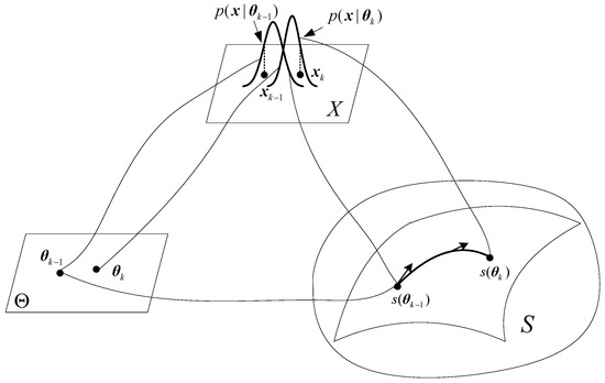
Figure 1.
Definition of a statistical manifold.
(2) Fisher information metric: The metric is the object specifying the scalar product in a particular point on a manifold in differential geometry. It encodes how to measure distances, angles and area at a particular point on the manifold by specifying the scalar product between tangent vectors at that point [25]. For a parameterized family of probability distributions on a statistical manifold, the FIM plays the role of a Riemannian metric tensor [1]. Denoted by , where
the FIM measures the ability of the random variable to discriminate the values of the parameter from for close to .
(3) Affine connection and Flatness: The affine connection ∇ (The notation ∇ is also used to denote the Jacobian in this paper. However, there should be no confusion from the context.) on a manifold S defines a linear one-to-one mapping between two neighboring tangent spaces of the manifold. When the connection coefficients of ∇ with respect to a coordinate system of S are all identically 0, then ∇ is said to be flat, or alternatively, S is flat with respect to ∇. The curvature of a flat manifold is zero everywhere. Correspondingly, flatness will result in considerable simplification of the geometry. Intuitively, a flat manifold is one that “locally looks like” a Euclidean space in terms of distances and angles. Consequently, many operations on the flat manifold such as projection and orthogonality become more closely analogous to the case of an Euclidean space.
It is worth mentioning that the flatness of a manifold is closely related to the definition of affine connections as well as the choice of coordinate systems of the manifold. In 1972, Chentsov [2] introduced a one-parameter family of affine connections called -connections which were later popularized by Amari [5]:
where
In Equation (20), = 0 corresponds to the Levi-Civita connection (information connection). The case = −1 defines the e-connection (exponential connection) while = −1 defines the m-connection (mixture connection). An exponential family with natural parameter as the coordinate system (parameterization) is a flat manifold under the e-connection while a mixture family with expectation parameter as the coordinate system is a flat manifold under the m-connection [24]. The e-connection and m-connection play an important role in statistical inference and geometrize the estimation on the flat manifolds.
3.2. Information Geometric Interpretation for Natural Gradient MLE
Based on the principles of information geometry introduced above, the algorithm described in Algorithm 1 can be explained via Figure 2, where the upper figure illustrates the estimation operation in Euclidean space while an alternative view of the estimation operation on statistical manifolds is analogously illustrated in the lower figure. In the upper figure, the local parameter is to be estimated from measurements (samples) via the likelihood function . When the measurement model is nonlinear in the parameter, the underlying estimation of the local parameter is a nonlinear estimation or filtering problem. Usually, linear signal processing problems can be routinely solved systematically by the astute application of results from linear algebra. However, the nonlinear cases are not easy to solve. The methodology of differential and information geometry are more adaptable and capable of dealing with nonlinear problems.
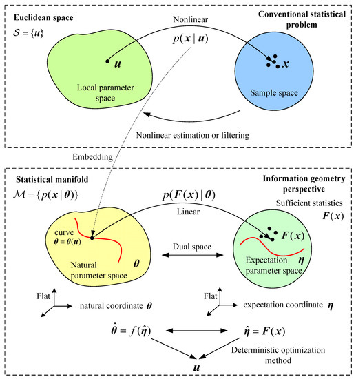
Figure 2.
Illustrates the nonlinear estimation concept in both Euclidean space and statistical manifolds of the dual spaces of natural parameter and expectation parameter . Top figure shows relations between parameter spaces (left) and samples (right) and associated estimating mappings. Bottom figure shows equivalent model for manifolds of parameter (left) and sample distributions (right). In both cases, the aims are to estimate the most likely parameter values that predict the data, and vice-versa.
Given that signifies a general set of conditional distributions, the natural parameter space contains the distributions of all exponential families; to be regarded as an enveloping space. Then the curved exponential family in the upper figure is smoothly embedded in the enveloping space by distribution reparameterization , i.e., the curved exponential family can be represented by a curve embedded in . Consequently the nonlinearity in the underlying estimation problem is completely characterized by the red curve inside the natural parameter space.
The circle on the lower right side of Figure 2 is the expectation parameter space or sampling space, which is dual to the natural parameter space . The dots in the space signify the “realizations” of the sufficient statistics of the distribution and they are obtained from measurements (samples) . Connected by the Legendre transformation the dual enveloping sub-manifolds and (i.e., natural and expectation parameter spaces) are in one-to-one correspondence [5]. By viewing the expression of the curved exponential families in Equation (1), we observe that the newly formulated likelihood is linear, which indicates the possibility for linearly estimating the natural parameter by sufficient statistics firstly and then obtaining the estimation of local parameter by a deterministic mapping from to .
The nonlinear filtering is performed in the expectation parameter space by projecting the samples on to the sub-manifold represented by the red curve which signifies the embedding of the curved exponential families in . The process is also called m-projection. As mentioned earlier, under both the e- and m-connections, the dual enveloping manifolds are flat. Therefore, the filtering (m-projection) is analogous to the projection in a deterministic Euclidean space. In consequence, the nonlinear estimation problem is finally realized as a deterministic optimization method.
The fundamental difference between the filter described here and existing nonlinear filters is that the filtering process presented is performed linearly in the dual spaces of natural parameters and expectation parameters under e- and m-connections, respectively. The filtering outcome is then mapped to local parameter space. The estimator is optimal in the MLE sense and thus has no information loss in the filtering process since it attains the CRLB [5].
The convergence of the nonlinear iterative estimator can be geometrically explained in information geometric terms diagrammatically via Figure 3. The curved exponential family in Equation (1) is represented by the curve in and also by in the dual space . Starting from an initial parameter , the algorithm constructs a vector from the current distribution represented by its expectation parameter to the measurement . The projection of to the tangent vector of the natural parameter with respect to the metric gives the steepest descent gradient (natural gradient) to update the current estimates (where is represented by the dashed arrow in both and , while the natural gradient is represented by the solid arrow in ).
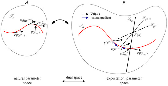
Figure 3.
Convergence of the presented iterative maximum likelihood estimator (MLE) algorithm.
The iterations continue according to Equation (16) until the two vectors and are (approximately) orthogonal to each other, i.e., . The algorithm achieves convergence with the steepest descent gradient vanishes and a solution to the MLE Equation (13) is obtained by projecting the data onto orthogonally to .
- Statistical problems can be described in manifolds in a number of ways. In the parameter estimation problems as we have discussed here the parameter belongs to a curved manifold, whereas the observations may lie on an enveloping manifold. The filtering process is thus implemented by means of projection in the manifolds.
- The iterative estimator is optimal in the MLE sense as the filtering itself involves no information loss. The stochastic filtering problem becomes an optimization problem defined over a statistical manifold.
- As seen from Algorithm 1, the algorithm implementation is relatively simple and straightforward by distribution reparameterization and operating in the dual flat manifolds. Though a Newton method-based MLE estimator can be derived directly via the likelihood. However, in most cases the operation is not trivial.
- The initial guess is important to facilitate convergence of the estimator to the true value. This can be varied and such initial value sampling may provide more certainty about reaching a global minimum. This has not been examined here.
In the next section, two examples are given to demonstrate the implementation of the developed estimator as well as its geometric interpretation.
4. Examples of Implementation of Natural Gradient MLE
4.1. An One Parameter Estimation Example of Curved Gaussian Distribution
Consider a curved Gaussian distribution
where a is a constant and u is an unknown parameter to be estimated. The collection of distributions specified by the parameter u constitute a one-dimensional curved exponential family, which can be embedded in the natural parameter space in terms of natural coordinates
which is a parabola (denoted by )
in . The underlying distribution in Equation (22) can be alternatively embedded in the expectation parameter space in terms of expectation coordinates
which is also a parabola (denoted by )
in .
The tangent vector of the curve is
The metric has only one component g in this case, and is
The sufficient statistics of the underlying distribution are
and they are obtained from measurements (samples) x.
Figure 4 shows the two dual flat spaces ( and ) and illustrates the estimation process implemented in them, where the blue parabolas in two figures denote the embeddings of the curved Gaussian distribution specified by parameter u. Without loss of generality, are assumed. The red arrows in two figures show the tangent vector of the curve while the two red dots on the parabolas denote the “realizations” of the distribution in Equation (22) specified by the given parameter . One hundred observed data (measurements) are shown by the blue dots in the expectation parameter space specified by coordinates . The red asterisk denotes the sufficient statistics obtained from the statistical mean of the measurements (samples). By projecting the data on to the sub-manifold represented by orthogonally to , i.e., , the MLE estimation of parameter u is obtained. By viewing Equation (25) and Figure 4b, the estimation is with high accuracy to the true value of u in this example.
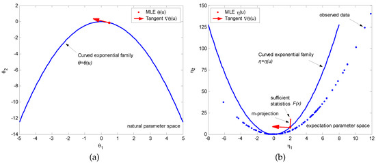
Figure 4.
Estimation example of one-dimensional curved Gaussian distribution. (a) Shows the natural parameter space and embedding of the curved Gaussian distribution in it; (b) Shows the dual expectation parameter space and the estimation process in it.
4.2. A Mote Localization Example via RIPS Measurements
The Radio Interferometric Positioning System (RIPS) is an efficient sensing technique for sensor networks of small, low cost sensors with various applications. It utilizes radio frequency interference to obtain a sum of distance differences between the locations of a quartet of the motes which is initially reported in [26] and further discussed in [27]. In this paper, we take this mote localization problem via RIPS measurements as an application of the presented natural gradient MLE.
(1) Problem description: The Radio Interferometric Positioning System (RIPS) measurement model is described in [28]. A single RIPS measurement, as described in [26], involves four motes. A mote is a node in a sensor network that is capable of performing some processing, gathering sensory information and communicating with other connected nodes in the network. The main components of a sensor mote are a microcontroller, transceiver, external memory, power source and sensing hardware device. Figure 5 illustrates a collection of four motes , where and C are anchor motes (i.e., their location states are already known) and D is a free mote with unknown location. Two motes act as transmitters, sending a pure sine wave at slightly different frequencies. This results in an interference signal at a low beat frequency that is received by the other two motes (acting as receivers). A sum of range differences between the four motes can be obtained from the phase difference of the received interference signals at the two receiver locations. If motes A and B serve as transmitters and motes C and D form the receiver pair, then the corresponding RIPS measurement, denoted , measures the distance differences
which may be simply written as
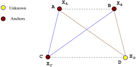
Figure 5.
Radio Interferometric Positioning System (RIPS) measurement involving four sensors with three known anchors and one unknown sensor.
In the absence of noise, two independent RIPS measurements can be found. Therefore, the other independent measurement is given by
which uses motes A and C as a transmitter pair and B and D as a receiver pair.
The two independent RIPS measurements can be written as
where is the unknown location of the free node D, and
are both known constants in which are the location coordinates of the three anchor motes.
Accordingly, a generic RIPS measurement model can be written as
The underlying localization problem is to estimate the location of the free mote D based on RIPS measurement in Equation (34), where we assume that the knowledge of anchor node locations are known. The problem of locating the node D from RIPS measurements corrupted with Gaussian noise in Equation (34) reduces to a nonlinear parameter estimation problem. We adopt the natural gradient based MLE estimator described above to address it.
(2) Mote localization via RIPS measurements: Based on the RIPS measurement model in Equation (34), we can write the likelihood function in the form
Rearranging Equation (35) to describe in terms of the canonical curved exponential family, we obtain
which yields (The required quantities can be obtained directly from the standard relations between Equations (4)–(7) for curved Gaussian distributions.)
The expectation parameter and FIM on natural parameter are given by
The Jacobian matrix of natural parameter with respect to local parameter is given by
where
The FIM with respect to the local parameter , i.e., Equation (15) becomes
Therefore, the iterative MLE estimator for estimating the location of a free mote using RIPS measurements is implemented as
The covariance of the estimator is the inverse of the Fisher information matrix given in Equation (49).
As with other gradient optimization algorithms, a reasonable guess of the initial state value is required to facilitate the optimization converges to the correct local minimum. In this application, the initial state may be obtained from the RIPS measurements via the RIPS trilateration algorithm described in [29], which is then used to calculate .
The performance of the proposed localization algorithm is illustrated by analyzing a scenario illustrated in Figure 6. In this example, three RIPS nodes are located at , , and m. The noise of a RIPS measurement is assumed to be zero-mean Gaussian with a standard deviation m.
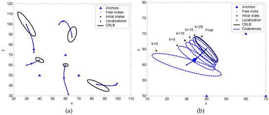
Figure 6.
(a) Shows how the algorithm correctly localizes 5 unknown sensors (“+”) from 3 motes (“”) with the iteration beginning at initial (guessed) locations; (b) Shows an example of the convergence of the iterative MLE estimator covariance to CRLB in the localization process.
Figure 6a shows 5 cases of localization results of the algorithm. The initial values are randomly generated in the simulations. We use the label CRLB to signify the ellipse which corresponds to the inverse of the Fisher information matrix of the network , centered at the true location . Figure 6b shows the covariances of the iterative MLE estimator at different iterations, where the kth error ellipse is calculated using the inverse of in Equation (49) and is centered at . Figure 7a,b demonstrate the localization results of different initial state values with the same measurements and results based on a set of measurements with the same initial state values, respectively. The estimator performance under this scenario is summarized in Table 1.
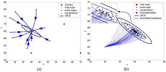
Figure 7.
(a) An example of localization with the same three anchor motes as in Figure 6 for iteration beginning at 10 different initial locations; (b) Localization results for a set of measurements with the same initial state values.

Table 1.
Estimator performance summary for the mote localization scenario shown in Figure 7b.
5. Conclusions
In this paper, an iterative maximum likelihood estimator based on the natural gradient method is described to address a class of nonlinear estimation problems for distributions of curved exponential families. We show that the underlying nonlinear stochastic filtering problem is solved by a natural gradient optimization technique which operates over statistical manifolds under dual affine connections. In this way, information geometry offers an interesting insight into the natural gradient algorithm and connects the stochastic estimation problem to a deterministic optimization problem. In this respect, the underlying philosophy is far more significant than the algorithm itself. Furthermore, based on an information geometric analysis it is promising that better algorithms for solving non-linear estimation problems can be derived. For instance, a “whitened gradient” which whitens the tangent space of a manifold has been presented in [30]. The whitened gradient replaces the Riemannian metric in the natural gradient updates by its square root and results in a faster and more robust convergence.
The work in this paper indicates that the methods of differential/information geometry provide useful tools for systematically solving certain non-linear problems commonly encountered in signal processing. Future work involves extrapolation of these techniques to handle the filtering problem for nonlinear stochastic dynamics.
Acknowledgments
This work was supported in part by the U.S. Air Force Office of Scientific Research under grant No. FA9550-12-1-0418.
Author Contributions
Yongqiang Cheng put forward the original ideas and performed the research. Xuezhi Wang conceived and designed the application of the estimator to RIPS mote network localization. Bill Moran reviewed the paper and provided useful comments. All authors have read and approved the final manuscript.
Conflicts of Interest
The authors declare no conflict of interest.
References
- Rao, C.R. Information and accuracy attainable in the estimation of statistical parameters. Bull. Calcutta Math. Soc. 1945, 37, 81–91. [Google Scholar]
- Chentsov, N.N. Statistical Decision Rules and Optimal Inference; Leifman, L.J., Ed.; Translations of Mathematical Monographs; American Mathematical Society: Providence, RI, USA, 1982; Volume 53. [Google Scholar]
- Efron, B. Defining the curvature of a statistical problem (with applications to second order efficiency). Ann. Stat. 1975, 3, 1189–1242. [Google Scholar] [CrossRef]
- Efron, B. The geometry of exponential families. Ann. Stat. 1978, 6, 362–376. [Google Scholar] [CrossRef]
- Amari, S. Differential geometry of curved exponential families-curvatures and information loss. Ann. Stat. 1982, 10, 357–385. [Google Scholar] [CrossRef]
- Amari, S.; Nagaoka, H. Methods of Information Geometry; Kobayashi, S., Takesaki, M., Eds.; Translations of Mathematical Monographs; American Mathematical Society: Providence, RI, USA, 2000; Volume 191. [Google Scholar]
- Amari, S. Information geometry of statistical inference—An overview. In Proceedings of the IEEE Information Theory Workshop, Bangalore, India, 20–25 October 2002. [Google Scholar]
- Smith, S.T. Covariance, subspace, and intrinsic Cramér–Rao bounds. IEEE Trans. Signal Process. 2005, 53, 1610–1630. [Google Scholar] [CrossRef]
- Srivastava, A. A Bayesian approach to geometric subspace estimation. IEEE Trans. Signal Process. 2000, 48, 1390–1400. [Google Scholar] [CrossRef]
- Srivastava, A.; Klassen, E. Bayesian and geometric subspace tracking. Adv. Appl. Probab. 2004, 36, 43–56. [Google Scholar] [CrossRef]
- Bhattacharya, R.; Patrangenaru, V. Nonparametric estimation of location and dispersion on Riemannian manifolds. J. Stat. Plan. Inference 2002, 108, 23–35. [Google Scholar] [CrossRef]
- Richardson, T. The geometry of turbo-decoding dynamics. IEEE Trans. Inf. Theory 2000, 46, 9–23. [Google Scholar] [CrossRef]
- Ikeda, S.; Tanaka, T.; Amari, S. Information geometry of turbo and low-density parity-check codes. IEEE Trans. Inf. Theory 2004, 50, 1097–1114. [Google Scholar] [CrossRef]
- Haenggi, M. A geometric interpretation of fading in wireless networks: Theory and application. IEEE Trans. Inf. Theory 2008, 54, 5500–5510. [Google Scholar] [CrossRef]
- Westover, M.B. Asymptotic geometry of multiple hypothesis testing. IEEE Trans. Inf. Theory 2008, 54, 3327–3329. [Google Scholar] [CrossRef]
- Li, Q.; Georghiades, C.N. On a geometric view of multiuser detection for synchronous DS/CDMA channels. IEEE Trans. Inf. Theory 2000, 46, 2723–2731. [Google Scholar]
- Cheng, Y.; Wang, X.; Moran, B. Sensor network performance evaluation in statistical manifolds. In Proceedings of the 13th International Conference on Information Fusion, Edinburgh, UK, 26–29 July 2010. [Google Scholar]
- Cheng, Y.; Wang, X.; Caelli, T.; Li, X.; Moran, B. On information resolution of radar systems. IEEE Trans. Aerosp. Electron. Syst. 2012, 48, 3084–3102. [Google Scholar] [CrossRef]
- Wang, X.; Cheng, Y.; Moran, B. Bearings-only tracking analysis via information geometry. In Proceedings of the 13th International Conference on Information Fusion, Edinburgh, UK, 26–29 July 2010. [Google Scholar]
- Wang, X.; Cheng, Y.; Morelande, M.; Moran, B. Bearings-only sensor trajectory scheduling using accumulative information. In Proceedings of the International Radar Symposium, Leipzig, Germany, 7–9 September 2011. [Google Scholar]
- Altun, Y.; Hofmann, T.; Smola, A.J.; Hofmann, T. Exponential families for conditional random fields. In Proceedings of the 20th Annual Conference on Uncertainty in Artificial Intelligence, Banff, AB, Canada, 7–11 July 2004. [Google Scholar]
- Amari, S.; Douglas, S.C. Why natural gradient? In Proceedings of the IEEE International Conference on Acoustics Speech Signal Process, Seattle, WA, USA, 12–15 May 1998. [Google Scholar]
- Manton, J.H. On the role of differential geometry in signal processing. In Proceedings of the IEEE International Conference on Acoustics Speech Signal Process, Philadelphia, PA, USA, 18–23 March 2005. [Google Scholar]
- Amari, S. Information geometry on hierarchy of probability distributions. IEEE Trans. Inf. Theory 2001, 47, 1701–1711. [Google Scholar] [CrossRef]
- Brun, A.; Knutsson, H. Tensor glyph warping-visualizing metric tensor fields using Riemannian exponential maps. In Visualization and Processing of Tensor Fields: Advances and Perspectives, Mathematics and Visualization; Laidlaw, D.H., Weickert, J., Eds.; Springer: Berlin, Germany, 2009. [Google Scholar]
- Maroti, M.; Kusy, B.; Balogh, G.; Volgyesi, P.; Molnar, K.; Nadas, A.; Dora, S.; Ledeczi, A. Radio Interferometric Positioning; Tech. Rep. ISIS-05-602; Institute for Software Integrated Systems, Vanderbilt University: Nashville, TN, USA, 2005. [Google Scholar]
- Kusy, B.; Ledeczi, A.; Maroti, M.; Meertens, L. Node-density independent localization. In Proceedings of the 5th International Conference on Information Processing in Sensor Networks, Nashville, TN, USA, 19–21 April 2006. [Google Scholar]
- Wang, X.; Moran, B.; Brazil, M. Hyperbolic positioning using RIPS measurements for wireless sensor networks. In Proceedings of the 15th IEEE International Conference on Networks (ICON2007), Adelaide, Australia, 19–21 November 2007. [Google Scholar]
- Scala, B.F.; Wang, X.; Moran, B. Node self-localisation in large scale sensor networks. In Proceedings of the International Conference on Information, Decision and Control (IDC 2007), Adelaide, Australia, 11–14 February 2007. [Google Scholar]
- Yang, Z.; Laaksonen, J. Principal whitened gradient for information geometry. Neural Netw. 2008, 21, 232–240. [Google Scholar] [CrossRef] [PubMed]
© 2017 by the authors. Licensee MDPI, Basel, Switzerland. This article is an open access article distributed under the terms and conditions of the Creative Commons Attribution (CC BY) license (http://creativecommons.org/licenses/by/4.0/).