Extraction of the Proton and Electron Radii from Characteristic Atomic Lines and Entropy Principles


1
Faculty of Chemical Engineering, Central University of Ecuador, 170521 Quito, Ecuador
2
Sciences Technologies et Sante (STS), Université Paul Sabatier, 31062 Toulouse, France
*
Author to whom correspondence should be addressed.
Entropy 2017, 19(7), 293; https://doi.org/10.3390/e19070293
Submission received: 13 April 2017
/
Revised: 8 June 2017
/
Accepted: 9 June 2017
/
Published: 29 June 2017
(This article belongs to the Special Issue Quantum Mechanics: From Foundations to Information Technologies)
Abstract
:We determine the proton and electron radii by analyzing constructive resonances at minimum entropy for elements with atomic number Z ≥ 11.We note that those radii can be derived from entropy principles and published photoelectric cross sections data from the National Institute of Standards and Technology (NIST). A resonance region with optimal constructive interference is given by a principal wavelength λ of the order of Bohr atom radius. Our study shows that the proton radius deviations can be measured. Moreover, in the case of the electron, its radius converges to electron classical radius with a value of 2.817 fm. Resonance waves afforded us the possibility to measure the proton and electron radii through an interference term. This term, was a necessary condition in order to have an effective cross section maximum at the threshold. The minimum entropy means minimum proton shape deformation and it was found to be (0.830 ± 0.015) fm and the average proton radius was found to be (0.825 − 0.0341; 0.888 + 0.0405) fm.
1. Introduction
The so-called proton radius puzzle was born when electron scattering experiments or atomic spectroscopy gave different value for the radius of the proton when compared to a muonic experiment [1,2,3,4]. In the last experiment, the lamb shift was measured when the muon orbits a proton, allowing for a proton radius measurement. Other experiments included a Deuterium spectroscopy and muonic Helium. It was found in the former that the deuteron radius is smaller when measured in muonic deuterium, as compared to the average value using electronic deuterium [5,6,7]. There are also plans to simultaneously measure the scattering of electrons and muons at Muon Proton Scattering Experiment (MUSE) [3,6,7].
In light of modern quantum theory, the boundary of compact support of the mass distribution of a particle, just like the location of an electron, cannot be specified precisely. However, it is still advantageous to conceptualize an atomic system in classical terms, especially for specific energy environments wherein best-fit classical parameters are measured. The electrons in the atomic K-shell orbit much closer to the nucleus than other shells. At low energy (up to 0.116 MeV), it is well known that the photoelectric effect is more important than other effects for most elements on the periodic table [8], Figure 1, Figure 2, Figure 3 and Figure 4. We can see different peaks of photoelectric absorption being the strongest ones due to electrons located in the K-shell. Somehow, the system formed by electron, photon and nucleus interacts strongly in the K-shell when compared to other shells. The data base at the National Institute of Standards and Technology (NIST) [9] contains the tabulated photoelectric peak cross sections for every element on the periodic table. Resonance is a very general phenomenon in nature, but many times, we seem to ignore its existence. Resonance is discoverable when the energy in a system changes at a particular rate [10,11]. Using NIST published data and entropy principles, we developed a model for the atomic resonances of the electron, proton and photon systems (see Figure 1). Atomic resonances were completely identified through an interference term that became part of the model, and allowed us to measure the proton radius. Our model predicts that the proton is not a sphere, but rather an ellipse, which is in agreement with other experiments done by other laboratories [3,4,6,7]. The present work is an attempt to reconcile published muonic hydrogen and electron scattering data.
This paper is a generalization of the Bragg’s law of diffraction to a nuclear level, since it has an atomic foundation. We incorporated probability theory together with cross sections and found that a resonance wavelength allows us to obtain the proton and electron radii. The traditional Bragg’s law, which has an atomic range, contributed to the science of X-rays crystallography and solid state materials. The Bragg’s law will help us to study the surface and nuclear structure.
Our study of minimum entropy is based on the distribution of scattering cross section areas of systemic atomic resonances, or more specifically, K-shell resonances. During those resonances we have an optimal transfer of the energy at minimum entropy. From the analysis of our results, we can conclude that a stable atom has evolved, or is equivalent to a state of minimum entropy. In fact, according to the Kakutani fixed point theorem, we can consider that each stable atom has its own fixed point. Small perturbations, like the photoelectric effect, may disturb the atom. Depending on the nature of the perturbation, the atom or system will either return to the original stable state, or it will divert and wander off, until a new fixed point is encountered. Evolution is then the process of moving to a more stable fixed point, through random perturbations, due to the quantum nature of the universe.
The quantum minimum entropy, according to Von Neumann, occurs in a coherent state that satisfies equality in the Heisenberg uncertainty principle, which is as follows: ∆x. ∆p = h/2π and ∆E. ∆t = h/2π. Since each fixed point of a system is dynamic and always affected by random perturbations, we can have stochastic fluctuations and expectation values with maximum probability around the fixed point. According to the Noether perspective, a fixed point implies symmetry, where some magnitude is conserved [12]. We can therefore generalize Noether’s theorem by saying, that at a fixed point, information is conserved and represents a state of minimum entropy. These concepts allow us to understand the boundary between classical and modern physics. For example, the de Broglie wavelength carries the minimum entropy regarding the information about the position and momentum. In the same way, Maxwell equations can be considered as the bridge between electromagnetic and quantum processes, only when everything happens at minimum entropy, or the information is conserved.
2. Theory
Resonance phenomena can be seen at low energy when X-rays interact with periodic table atoms. This is true when we analyze attenuation peaks, produced from low energy radiation interaction with matter [10,11], Figure 2, Figure 3 and Figure 4.
If we consider that resonance is a threshold phenomenon, we can find a specific wavelength λ where maximum energy is transferred from one photon to another electron or proton [10,11]. In our analysis, low energy X-rays interacted with the atomic structure as a system and produced resonances. We also saw minimum increases of energy that produced more than 250% of the photoelectric effect cross section (σm >> σm−1) for a time t = m, and for each atom of the periodic table. When we considered resonance threshold frequencies, we found that the maximum variation of the cross section was located where the energy variation was minimum Min(Em − Em−1) or equal to zero during the same time interval, as follows:
The resonance phenomenon is an optimal process [10,11], in the sense that entropy is minimized. During resonance, system entropy should be minimum and can be measured when huge increases of atomic cross sections are detected. This last aspect is the result of interference phenomena between the atomic nucleus, X-rays and atomic electrons [13,14,15,16,17,18].
In order to have a clear understanding of how this process occurs, we are going to explain each one of the events. Those events are ordered and optimized naturally, in such a way, that a maximum value of the cross section is obtained for every atom between: 11 ≤ Z ≤ 92.
- E1
- E2
- Constructive interference: There are constructive interferences among the X-rays and later on with the atomic nucleus or electron. This occurs only if ra ≈ rn + λ, where ra is the atomic radius and rn is the nucleus radius.
- E3
- E4
- The optimal cross section of the atomic nucleus depends on the proton radius rp. The proton radius will be measured indirectly through the atomic total cross section, which is a result of the interference between the nucleus (but always with a specific nucleon), X-rays and the electron [18].
3. Definitions
The atom will be characterized by the atomic radius ra, number of protons Z = A − N, number of electrons Z, and number of neutrons N.
Cross Section
According to NIST, current tabulations of μ/ρ rely heavily on theoretical values for the total cross section per atom, σtot, which is related to μ/ρ by the following equation:
In Equation (3), u (=1.6605402 × 10⁻²⁴ gr) is the atomic mass unit (1/12 of the mass of an atom of the nuclide 12C) [9].
The attenuation coefficient, photon interaction cross sections, and related quantities are functions of the photon energy. The total cross section can be written as the sum over contributions from the principal photon interactions:
where σpe is the atomic photo effect cross section; σcoh and σincoh are the coherent (Rayleigh) and the incoherent (Compton) scattering cross sections, respectively; σpair and σtrip are the cross sections for electron–positron production in the fields of the nucleus and of the atomic electrons, respectively; and σph.n. is the photonuclear cross section [9,20].
We use data from NIST for elements Z = 11 to Z = 92 and photon energies 1.0721 × 10⁻³ MeV to 1.16 × 10⁻¹ MeV, which have been calculated according to:
The probability of finding a proton inside the atom, and more specifically, inside the nucleus is given by Pn:
The probability of finding at least one electron inside the atom is represented by Bohr’s radius and is defined by:
where: ra is the atomic radius, re is the electron radius, rn is the nucleus radius, and rp is the proton radius.
4. Resonance Region
A resonance region is created in a natural way at the K-shell between the nucleus and the electrons at S-level. The condition for the photons to enter into the resonance region is given by ra ≥ rn + λ. This resonance region gives us a new way of understanding the photoelectric effect. There is experimental evidence of the existence of resonance at K-level due to the photoelectric effect, represented by the resonance cross section provided by NIST for each atom. In the present work, we focus on resonance effects, but not on the origin of the resonance region.
Shannon Entropy
We will use Shannon entropy S, in the traditional way, as used in Statistical Mechanics since the Boltzmann era, i.e., with natural logarithms.
In Information Theory we use the logarithms of base 2, to represent bits of information.
Both representations measure the state of evolution and order of the system. The entropy measures system characteristics, and system information. This description will be used in this paper. In summary, the entropy S represents the information and degree of order present in the physical system.
Shannon’s entropy S measures the information of a system and is given by:
In order to have minimum entropy [21,22,23,24,25,26,27], every part of the atom should have a shape and structure optimal in a way that the whole system works as one. The Equation (8) only depends on the nucleus radius. The minimum nucleus radius will be used rn* = rp A1/3 instead of the traditional nucleus radius given by rn* = 1.2 A1/3. This new equation can be obtained from the following volumetric relation:
The Equation (9) will be used in order to minimize the entropy.
Theorem 1.
The atom is a minimal entropy system.
The problem is solved using the KKT (Karush–Kund–Tucker) method [24,25,26,27]. The Lagrangian is built in a traditional way L = S + µ(pn + pe − 1) with the constraint µ(pn + pe − 1) = 0.
After solving the Lagrangian, dL/drp = 0, we obtain µ > 0 as follows:
Since µ > 0, we should have
This implies that the minimum of the entropy has a solution, since µ is larger than zero, and Equation (10) has the solution. In other words, rp exists in the interval from 0.83 fm to 0.88 fm for every one of the atoms. In summary, the entropy is minimum for the minimum radii.
Equation (12) depends on the radii of the electron and the nucleon. From this equation we can solve for the proton radius for each element of the periodic table. We then obtain the theoretical limit of the proton radius according to Figure 2.
Once the limits of the proton radius had been established we found that they were in agreement with experimental values. Therefore, we can find the proton radius value of minimum entropy by using the following equation.
Theorem 2.
Resonance region. The resonance cross section is produced by interference between the atomic nucleus and the incoming X-rays inside the resonance region, where the boundaries are the surface of the atomic nucleus and K-shell.
The cross section of the atomic nucleus is given by:
The photon cross section in the K-shell depends on the wave length and the shape of the atomic nucleus:
Subtracting the cross sections (14) and (15) we have:
The resonance is produced by interactions between the X-rays, the K-shell electrons and the atomic nucleus. The cross sections corresponding to the nucleus is weighted by probability pn and should have a simple dependence on an interference term. This last aspect depends on the proton radius rp, or the difference between the nucleus and proton radius (rn − rp), according to the following relation:
We note that the left sides of Equations (17) and (18) should have a factor larger than one, due to resonance. The unique factor that holds this requirement is (pn + pe)/pn.
Due to physical reasons, the term that should be taken is 4π(2rpλ) because this is the only term that is in the boundary of the resonance region.
The reason that the cross section proton should be elliptical is because we can only measure one axis of the ellipse, and current experimental values are in the range of 0.83 fm to 0.88 fm.
It should be noted that the X-rays interaction is with a given proton located at the nucleus boundary. Therefore, the semi-empirical version of the Equation (17), which has been validated using experimental data from NIST and theoretical foundations, is then given by:
From Equation (19) we obtain that proton dimensions are given by the two principal axes of an ellipse, where the proton radius is defined by the relation rp2 = ab.
We have therefore shown that we can verify Equation (19) using NIST data for each of the elements on the periodic table. The results for ellipse axis values and the proton radius [23] can be seen in Table 1.
The region of effective cross section is produced by the interference between the atomic nucleus, the electrons in the K-shell, and the X-rays trapped inside the resonance box or region.
The effective cross section due to the presence of the electron in the K-shell is given by:
The previous cross section is the result of interference between the atomic nucleus and an electron in the K-shell, after an X-ray is reflected from the nucleus surface. This last reaction creates an effective cross section, which is a function of the wavelength and electron physical size:
If we subtract the effective cross sections from Equations (20) and (21) we have:
The last relation shows the resonance effect that is produced when the X-rays interact with the electrons. We then have constructive resonances between the X-rays, the electrons in the K-shell and the atomic nucleus. The corresponding fraction for the electron effective resonance cross section is given by:
Theorem 3.
Electron and proton radii at minimum entropy.
Equation (17) shows that the cross section value of the electron (proton) could be the radius re or any one of the measured axis ai, bi that are positive random variables, where: i =1… n; re2 = ai bi.
Note that the axis and the cross section radius are variables that have quantum nature and are therefore treated as random variables.
If we consider that the electron radius is the geometric mean of the measured axis (ai, bi), then we can apply the central limit theorem. This theorem states that the probability law of any mean value follows a Gaussian law.
The entropy of a normal density probability is given as the natural logarithm of the standard deviation s. This implies that the minimum value of entropy for the electron radius represents the minimum value of the electron radius standard deviation, min(H) = min(s), where:
If the electron has an elliptical cross section, then the minimum value of electron (proton) entropy implies minimal deformation of its effective cross section.
The condition of standard deviation minimum value at Equation (26) is true if and only if the electron (proton) radius is the average value of the random variables ai y bi. It is not possible to distinguish between the major axis or minor axis, because when the random variable ai increases, the other random variable bi decreases, or vice versa.
From the experimental measurement of one of the axes of the measured ellipse, let us say bi, we can calculate the average value of the same axis. This last aspect represents the minimum entropy electron (proton) radius.
The value of the other axis ai is obtained from the following equation valid for i = 1…n:
The Equations (27) and (28) guaranteed that the standard deviation s(re) have a minimum value.
We note that a simultaneous measurement of the random variables ai, bi is not allowed by the uncertainty principle. Therefore, it is not possible for a straightforward measurement of the electron (proton) radius to occur, if the cross section has been deformed.
The measurement the electron (proton) radius is only possible when there is no deformation [14,15]. This last statement is true, if for every i = 1…n, we have:
During the time we measured the random variable bi, we introduced a perturbation in the momentum particle in the direction bi given by spb. This last action created another perturbation in the variable ai.
It raises the question of whether or not it is possible to represent the electron in the K-shell and the nucleon as a system in equilibrium. The answer comes from quantum games theory. In this theory, protons and electrons are related through strategies, the energy and system probability laws, as a whole, and they cannot be determined specifically inside the atom.
Theorem 4.
Electron radius is an equilibrium point.
Using Equation (17), it is easy to understand that the effective resonance cross section is a function of the interference term, due to the electron and proton, which are weighted by the probability and atomic weight relation. The close relation of Equations (23) and (24) is transformed into the following equalities:
Note that Equation (33) represents a fixed point, which is a requirement in Nash equilibrium. The term A is the atomic weight of the respective chemical element and AR corresponds to the reference atomic weight. This last aspect has a value with minimum error for the proton and/or electron radius.
The Equation (34) is explicit and it fixed point represents the electron radius re and has the following representation:
Once the electron radius is known, we can find the proton radius by using Equation (33). Note that if this equation holds for the electron, then its shape will be spherical.
The Equation (33) shows that the electron, and analogously, the proton, do not have a perfect spherical cross section. This is why the electron and proton radii cannot be measured and we can only distinguish one of the ellipse axes that represents the electron or the proton respectively.
The equations for the case that the electron and proton have an elliptical cross section, with axes be y bp, are respectively:
5. Discussion of Results
- The cross section for the proton is dynamic. The proton is deformed and increases with the atomic weight A, due to nuclear force. Using the minimum entropy theory, we can calculate the optimal dimension of the proton radius and the conditions for the photon to be trapped in the resonance region corresponding to the K-shell. Once in this region, the photon interacts with the electron or with one of the nucleons. In this paper, we give a calculation method for the proton radius as a function of the resonance cross section. However, in a similar way, we can also obtain the electron radius, since the low energy X-rays are confined to the boundaries corresponding to electrons in the K-shell and protons in the nucleus.
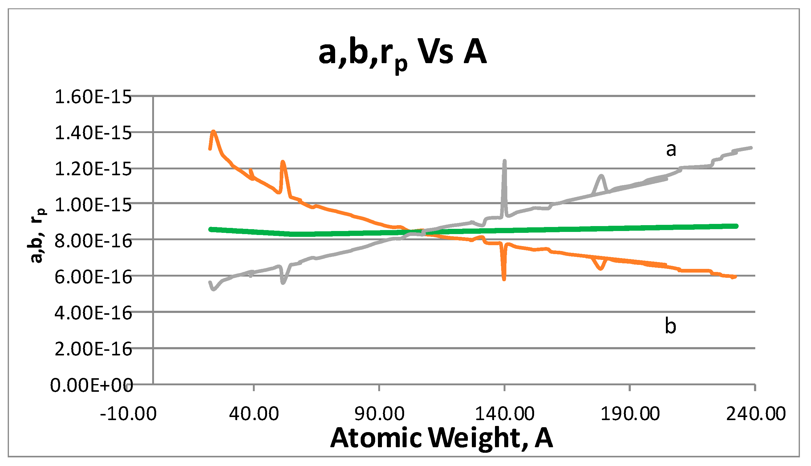
- The proton shape corresponds to a sphere with two different error measurements in length axis. From the experimental cross section, we can obtain two axes, the larger and the smaller. From the experiment we only obtain one axis, which is in the range of 1.3 fm ≤ b ≤ 0.59 fm, where 1.3 fm corresponds to sodium Z = 11 and 0.59 corresponds to Uranium Z = 92. We can calculate the second axis by using the formula rp2 = ab (Figure 3).
- Considering minimal deformation, the most probable value for the radius of the proton is obtained by averaging the measured value for one of its axes. The value obtained this way was 0.851 fm.
- This model allows us to explain the mass absorption curves for low energy X-rays and helps us to interpret the photoelectric effect in terms of the interference of wave properties. The question about why the K-shell has more probability than the more external ones, can be understood in terms of the effects of the nucleus in the resonance region, and the same for the electron. Moreover, the photons that come into the resonance region only have a small probability of producing a primary photoelectric effect, and for this reason, the secondary effect is predominant.
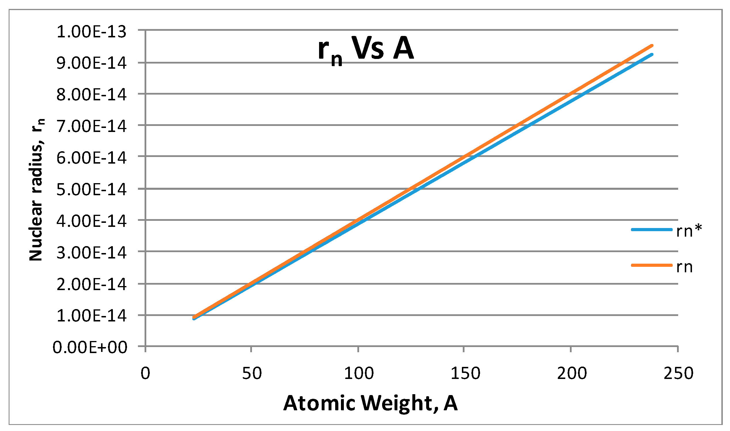
The solid rigid shape of the nucleus is completely known in terms of its radius, with a precision given by:
The Equation (38) gives the functional dependence the nucleus radius rn in terms of atomic number A, Figure 3. If we consider that the nucleons have a similar relationship, we then have:
However, from available experimental data we found that the range of variation of the proton radius is well below the corresponding nuclear radius.
According to our experimental values from Table 1, the value of one axis, with one standard deviation, is given by:
The scale of variation of our data is given in fm, which is within the range of other laboratories.
- 5.
We can see from Figure 5 the existence of a close relationship with Figure 4, which has been obtained from entropy principles only. This strongly suggest the idea of closed resonance regions inside the atoms.
The overlapping of the cross section for the nucleons is minimum, as we can see from the evolution of the probability interaction against the nucleus. This is a function of the atomic weight, Figure 6. This is true when we consider the empty space in the atomic nucleus. This space can be seen from the difference between the minimal nucleon radius and the known proton radius, given by Equation (24).
Electron Results: Discussion and Analysis
- The minimum entropy electron radius corresponds to the classical electron radius.
The classical electron radius, also known as Lorentz radius, is based on a classical relativistic model of the electron. Its value is 2.8179402894(58) fm.
- 1A.
- The meaning of Theorem 3. The electron is not a perfect sphere. The volumetric ellipse axes vary as a function of the atom and measurement where the electron is located. However, the electron radius converges to a value called minimum entropy. Such value is the geometric mean of the two axes of the effective cross section re2 = ai bi.
Experimentally, it is possible to find through NIST tables, for chemical elements 11 ≤ Z ≤ 92, the values of each of one of the axes for the proton. In this way, we can obtain the most probable value of (0.853 ± 0.201) fm. This last value corresponds, in a logical way, to the value of the electron classical radius 2817 fm. This last value is the one that is used as probability value.
- 1B.
- The second method to obtain the electron radius uses the same probability values that we found for the proton radius calculation. After using that information, we find the most probable value for the electron radius from Equations (33) and (34) and we get an experimental value in the range (2.75, 2.90) fm, Figure 7.
- 2.
- The interference of X-rays with the electron creates an effective resonance cross section. This last result depends on the electron radius, or any one of the ellipse axes, according to Equation (23). We have also analyzed the mass attenuation coefficients for elements with Z in the interval: 11 ≤ Z ≤ 92. The results are summarized in Table 1.
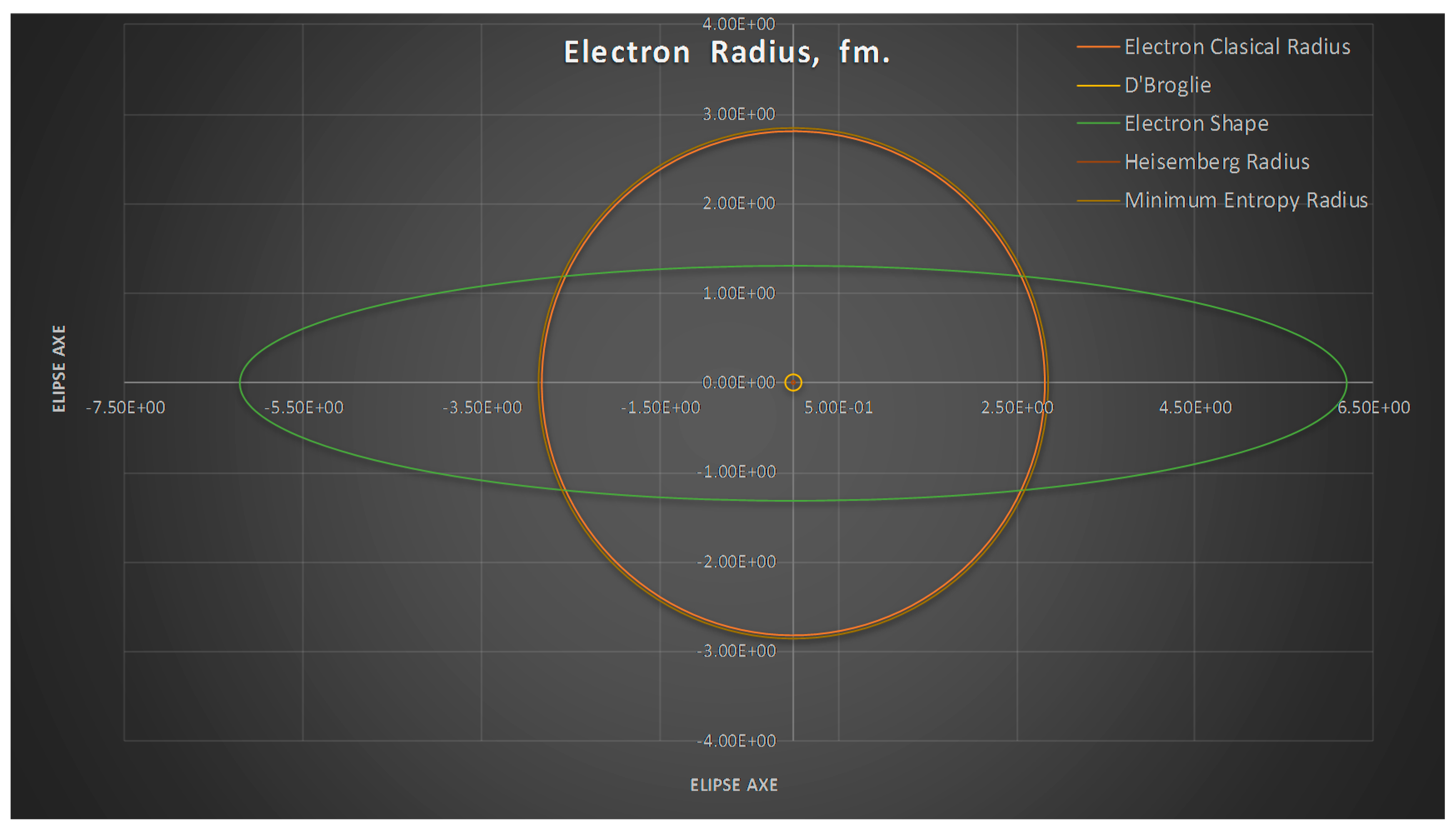
In Table 1 we calculated the minimum entropy electron radius, which was traduced in minimal deformation of the effective cross section. Once the other axis is obtained, we can make the following plots. They show the limits of the minimum entropy values, the electron classical radius, the Broglie wavelength corresponding to electron and the Heisenberg uncertainty principle.
- We can see from Figure 7 the spherical electron radius together with its deformed cross section. Note that we still see the electron as sphere even if its cross section is deformed.
- 3.
- The uncertainty principle is applied in its most rigorous way, as follows:
The product of the standard deviation in position times the standard deviation in momentum.
The standard deviation in momentum sp is calculated for each resonance energy. From Table 1 we will apply Equation (32).
We can see from Figure 8 that electron radius for minimum entropy can be obtained geometrically from the area of the deformed ellipse corresponding to the cross section.
Also, we can see from the chemical elements table, the values of the ellipse axes corresponding to the effective proton resonance cross section (Figure 9 and Figure 10).
- 4.
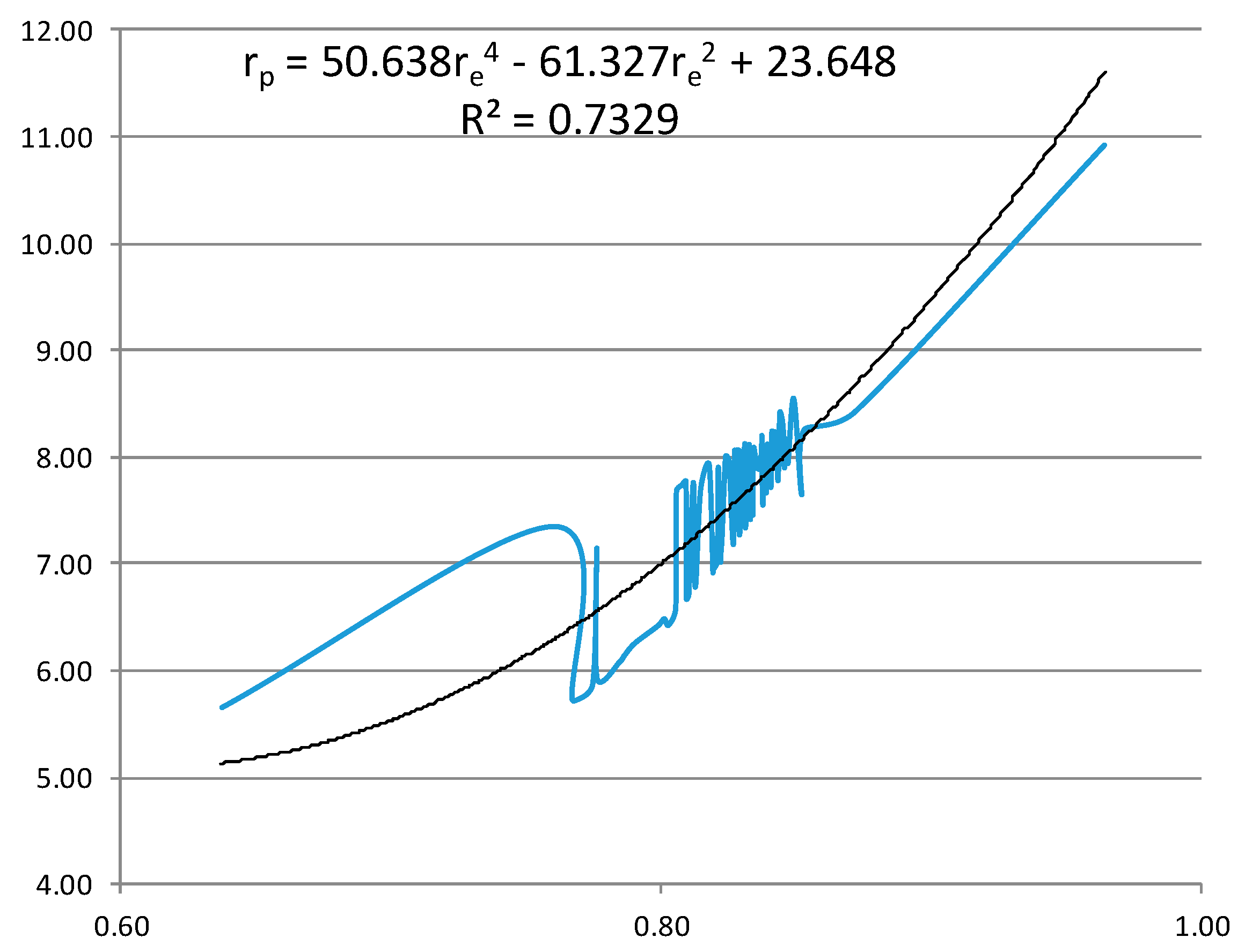
- From the experiment, the proton and electron radii have a functional relationship (Figure 11). It is found that the proton and electron radii are limited by the values of the two measured axes: (0.825 − 0341) fm < rp < (0.888 + 0.041) fm y (2.75 − 0.15) < re < (2.82 + 0.16) fm.
If we rewrite the Equation (34) then we have the functional dependence between the radii of the electron and the proton as follows:
6. Methods
We compiled all official information from the PML NIST division for elements from Z = 1 to Z = 92, for energies ranged (10 × 10−3 MeV to 1.16 × 10⁻¹ MeV), corresponding to the K-shell. Using the Equations (8)–(10), and (16) we obtained the final results reported in Table 2 and Table 3. Note that the photoelectric effect by resonance only starts to appear from Z = 11 to Z = 92.
7. Conclusions
We have presented a new method to extract the proton and electron radii by considering X-rays interference at low energy. Atomic resonances are only due to optimal interferences, which are maximum and occur at minimum entropy.
Our model predicts, within 5%, the theoretical electron radius and the inferred proton radius from recent reviews. During the analysis of atomic scattering data, we have assumed that the atom has spherical symmetry and disregarded states of non-zero angular momentum. We have also considered the proton and electron as classic particles with sharp edges, and used the term “orbit”, even though it cannot be specified with precision. According to our results, those assumptions work very well at the low energy range. More accurate scattering data will be necessary in order to refine the model.
In closing, it is important to describe future applications of this model, such as the “femtoscope”, which is a type of microscope that is able to measure items, up to the size of the nucleus, by using low energy probes. Another application to consider would be a better understanding of the absorbed radiation dose in tissues, also at low energy, which will enhance care management in cancer treatment.
Author Contributions
Edward Jiménez and Nicolas Recalde conceived the theoretical model. Esteban Jimenez Chacon processed data. Edward Jiménez and Nicolas Recalde wrote the manuscript. Both authors have read and approved the final manuscript.
Conflicts of Interest
The authors declare no conflict of interest.
References
- Jentschura, U.D. Muonic bound systems, virtual particles, and proton radius. Phys. Rev. A 2015, 92, 012123. [Google Scholar] [CrossRef]
- Pohl, R.; Antognini, A.; Nez, F.; Amaro, F.D.; Biraben, F.; Cardoso, J.M.R.; Covita, D.S.; Dax, A.; Dhawan, S.; Fernandes, L.M.P.; et al. The size of the proton. Nature 2010, 466, 213–216. [Google Scholar] [CrossRef] [PubMed]
- Strauch, S. Elastic Electron and Muon Scattering Experiment off the Proton at PSI. In Proceedings of the Particle and Nuclei International Conference 2014, Hamburg, Germany, 24–29 August 2014. [Google Scholar]
- Griffioen, K.; Carlson, C.; Maddox, S. Consistency of electron scattering data with a small proton radius. Phys. Rev. C 2016, 93, 065207. [Google Scholar] [CrossRef]
- Horbatsch, M.; Hessels, E.A.; Pineda, A. Proton radius from electron-scattering and chiral perturbation theory. Phys. Rev. C 2017, 95, 035203. [Google Scholar] [CrossRef]
- Kraus, E.; Mesick, K.E.; White, A.; Gilman, R.; Strauch, S. Polynomial fits and the proton radius puzzle. Phys. Rev. C 2014, 90, 045206. [Google Scholar] [CrossRef]
- Lee, G.; Arrington, J.R.; Hill, R.J. Extraction of the proton radius from electron-proton scattering data. Phys. Rev. D 2015, 92, 013013. [Google Scholar] [CrossRef]
- Olive, K.A. Review of Particle Physics (Particle Data Group). Chin. Phys. C 2014, 38, 090001. [Google Scholar] [CrossRef]
- Hubbell, J.H.; Seltzer, S.M. X-ray Mass Attenuation Coefficients, Radiation Division, PML, NIST, 2017. Available online: https://www.nist.gov/pml/x-ray-mass-attenuation-coefficients (accessed on 1 October 2016).
- Samuel, W. Introductory Nuclear Physics, 2nd ed.; Wiley-VCH Verlag GmbH & Co. KGaA: Weinheim, Germany, 2004. [Google Scholar]
- Mitchell, A.C.G.; Zemansky, M.W. Resonance Radiation and Exited Atoms; Cambridge University Press: Cambridge, UK, 2009. [Google Scholar]
- Christopher, G. Quantum Information Theory and the Foundation of Quantum Mechanics. Ph.D. Thesis, Oxford University, London, UK, 2004. [Google Scholar]
- Max, B. Atomic Physics, 2nd ed.; Blackie & Son Limited: London, UK, 1937. [Google Scholar]
- David, J.J. Classic Electrodynamics; John Wiley & Sons: Hoboken, NJ, USA, 2004. [Google Scholar]
- Landau, L.D.; Lifschitz, E.M. Mechanics; Nauka Publishers: Moscow, Russia, 1988. [Google Scholar]
- Claude, C.T. Quantum Mechanics; Wiley-VCH: Hoboken, NJ, USA, 1992. [Google Scholar]
- Sick, I. On the rms-radius of the proton. Phys. Lett. B 2003, 576, 62–67. [Google Scholar] [CrossRef]
- Briggs, J.S.; Lane, A.M. The effect of atomic binding on a nuclear resonance. Phys. Lett. B 1981, 106, 436–438. [Google Scholar] [CrossRef]
- Blunden, P.G.; Sick, I. Proton radii and two-photon exchange. Phys. Rev. C 2005, 72, 057601. [Google Scholar] [CrossRef]
- Griffits, D. Introduction to Elementary Particles, 2nd ed.; Wiley-VCH: Hoboken, NJ, USA, 2008. [Google Scholar]
- Karush, W. Isoperimetric Problems and Index Theorems in the Calculus of Variations. Ph.D. Thesis, Department of Mathematics, University of Chicago, Chicago, IL, USA, 1942. [Google Scholar]
- Fischer, M.; Kolachevsky, N.; Zimmermann, M.; Holzwarth, R.; Udem, T.; Hänsch, T.W.; Abgrall, M.; Grünert, J.; Maksimovic, I.; Bize, S.; et al. New limits on the drift of fundamental constants from laboratory measurements. Phys. Rev. Lett. 2004, 92, 230802. [Google Scholar] [CrossRef] [PubMed]
- Bliss, G.A. Lectures on the Calculus of Variations; University of Chicago Press: Chicago, IL, USA, 1946. [Google Scholar]
- Hestenes, M.R. Calculus of Variations and Optimal Control Theory; John Wiley & Sons: New York, NY, USA, 1966. [Google Scholar]
- Pars, L.A. An Introduction to the Calculus of Variations; John Wiley & Sons: New York, NY, USA, 1962. [Google Scholar]
- Karush, W. Mathematical Programming, Man-Computer Search and System Control; Technical Report SP-828; System Development Corporation: Santa Monica, CA, USA, 1962. [Google Scholar]
- Kuhn, H.W.; Tucker, A.W. Nonlinear programming. In Proceedings of the Second Berkeley Symposium on Mathematical Statistics and Probability, Statistical Laboratory of the University of California, Berkeley, CA, USA, 31 July–12 August 1950; Neyman, J., Ed.; University of California Press: Berkeley, CA, USA, 1951; pp. 481–492. [Google Scholar]
Figure 1.
The figures above show the resonance regions. Yellow means M shell, blue means L shell, and green K shell.
Figure 1.
The figures above show the resonance regions. Yellow means M shell, blue means L shell, and green K shell.
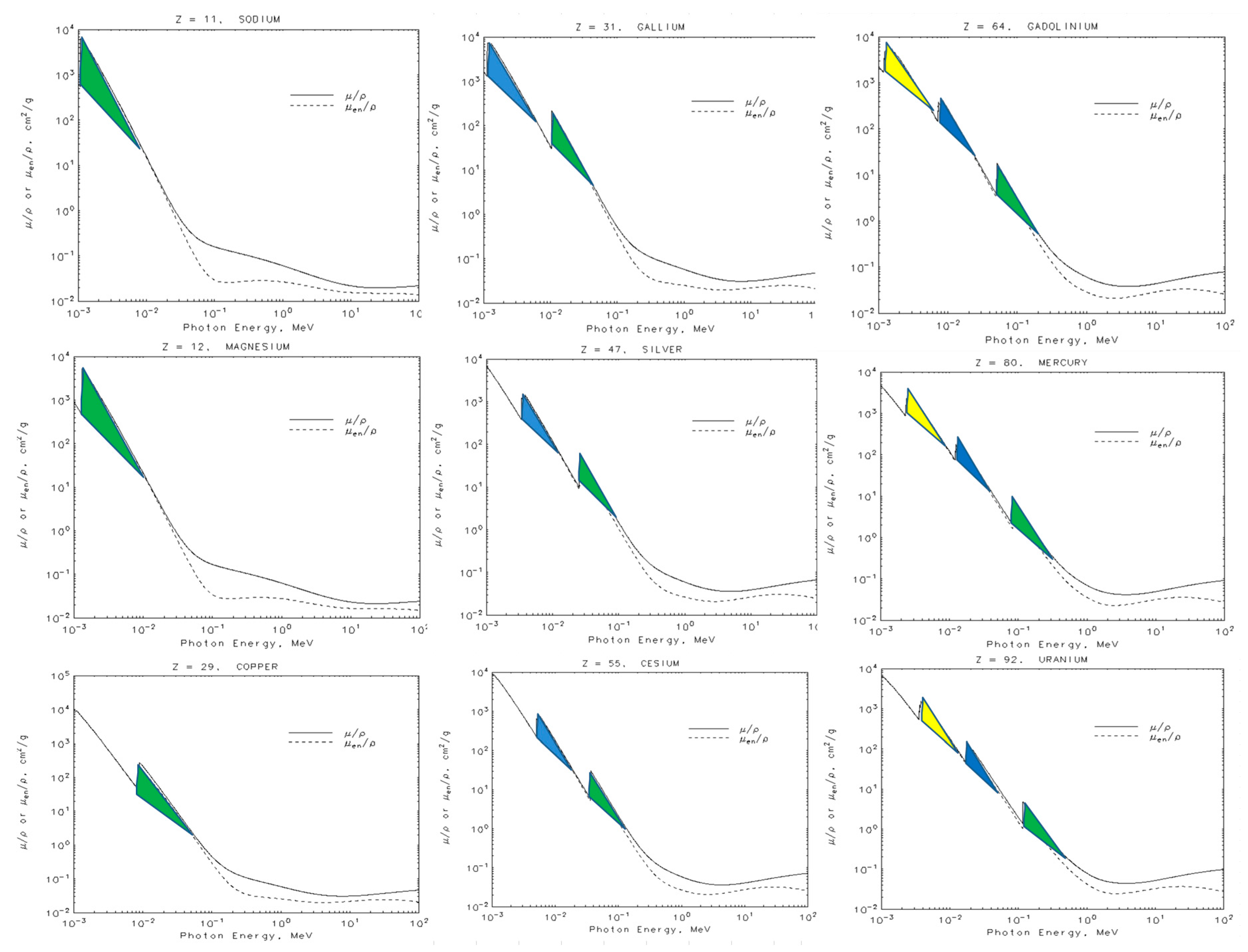
Figure 2.
Evolution of the proton’s size inside the nucleus. We can see how the proton radius varies as a function of Z, where Z = 11 to Z = 92.
Figure 2.
Evolution of the proton’s size inside the nucleus. We can see how the proton radius varies as a function of Z, where Z = 11 to Z = 92.
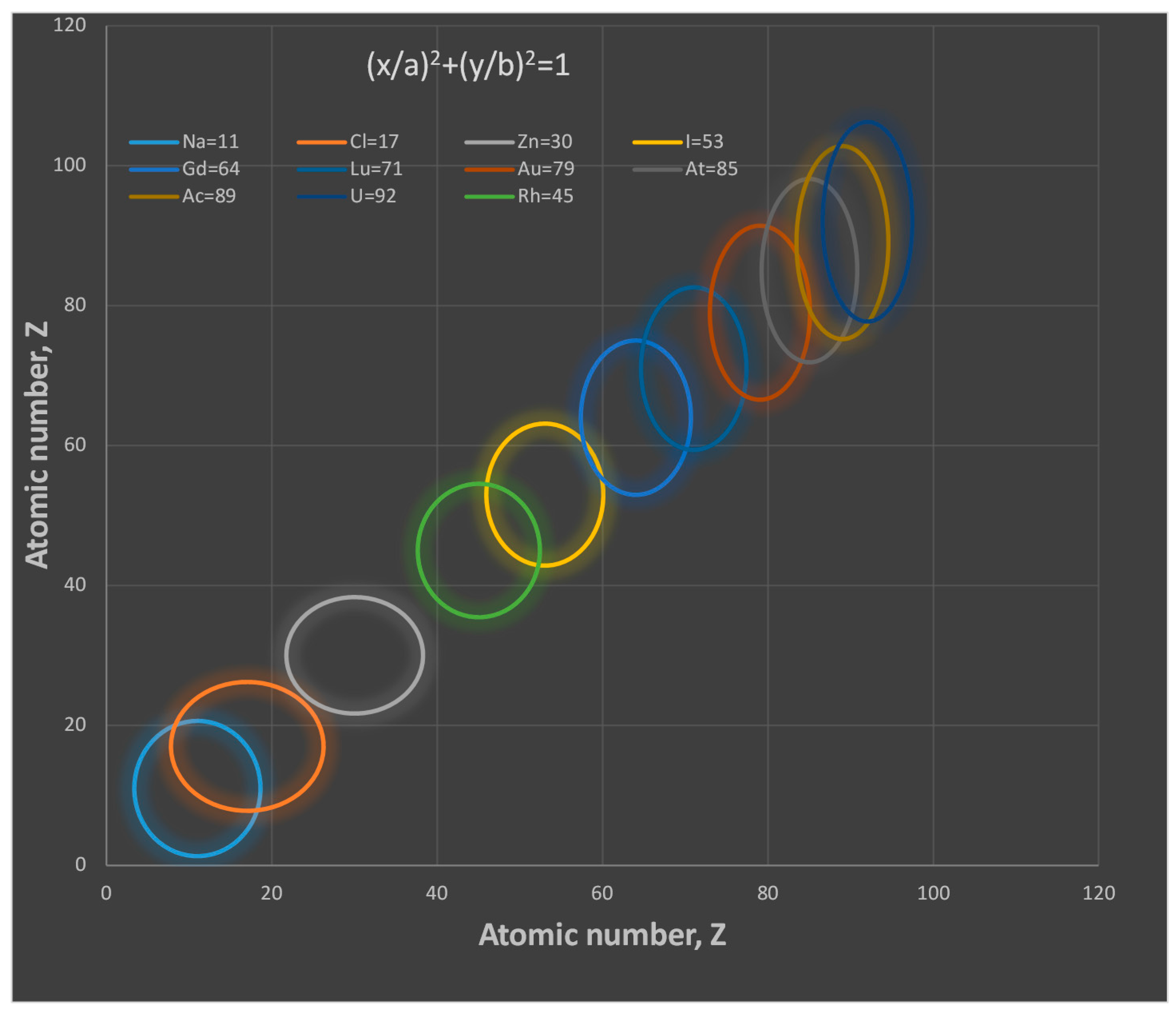
Figure 3.
Variation of nucleus radius for every atom of the periodic table, rn = rn(A). Blue represents theoretical value and orange represents experimental value.
Figure 3.
Variation of nucleus radius for every atom of the periodic table, rn = rn(A). Blue represents theoretical value and orange represents experimental value.

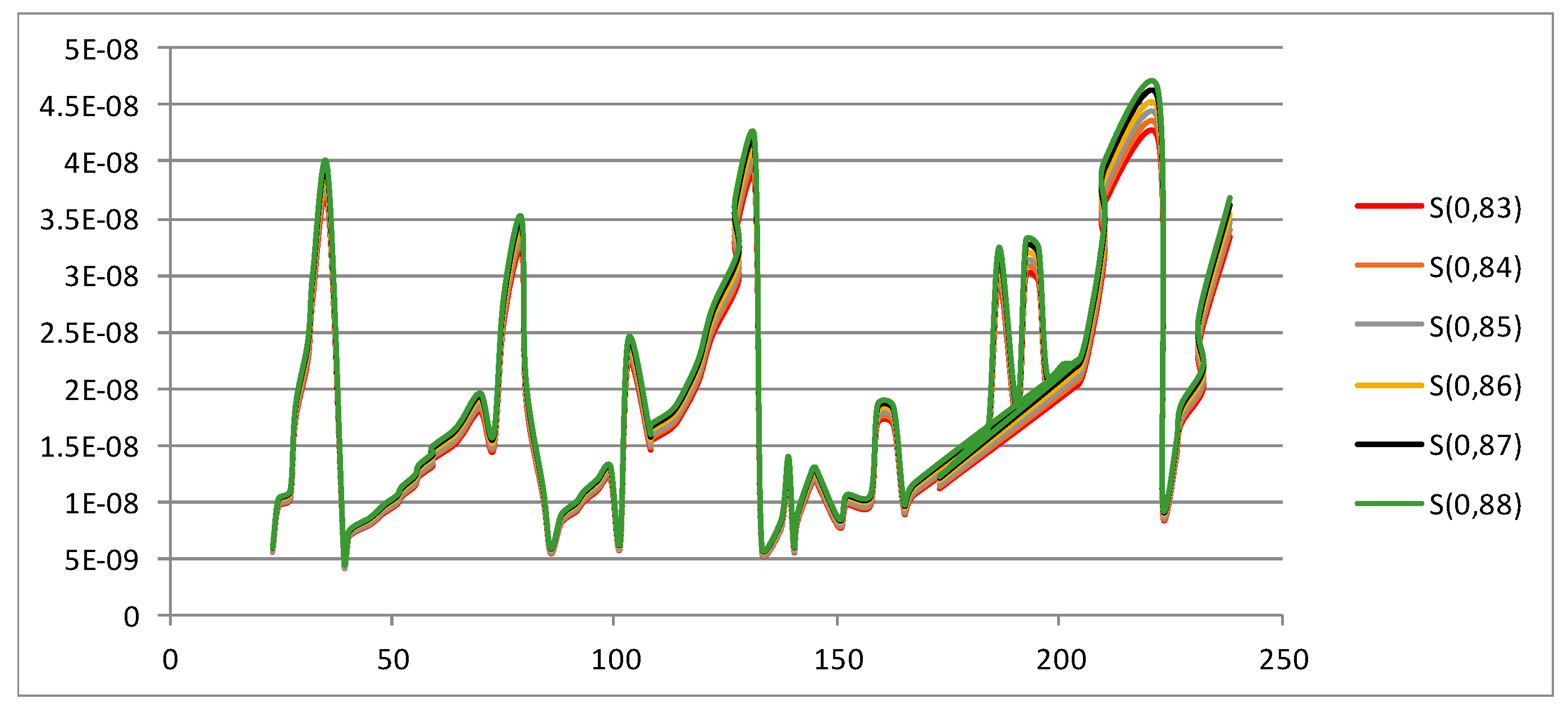
Figure 4.
The figure shows minimum entropy values for different elements of the periodic table where 11 ≤ Z ≤ 92. We can see that minimum entropy corresponds to a value of the proton radius equal to 0.83 fm. This result is in agreement with the experiments reported in the bibliography [2,3,4,5,6,7].

Figure 5.
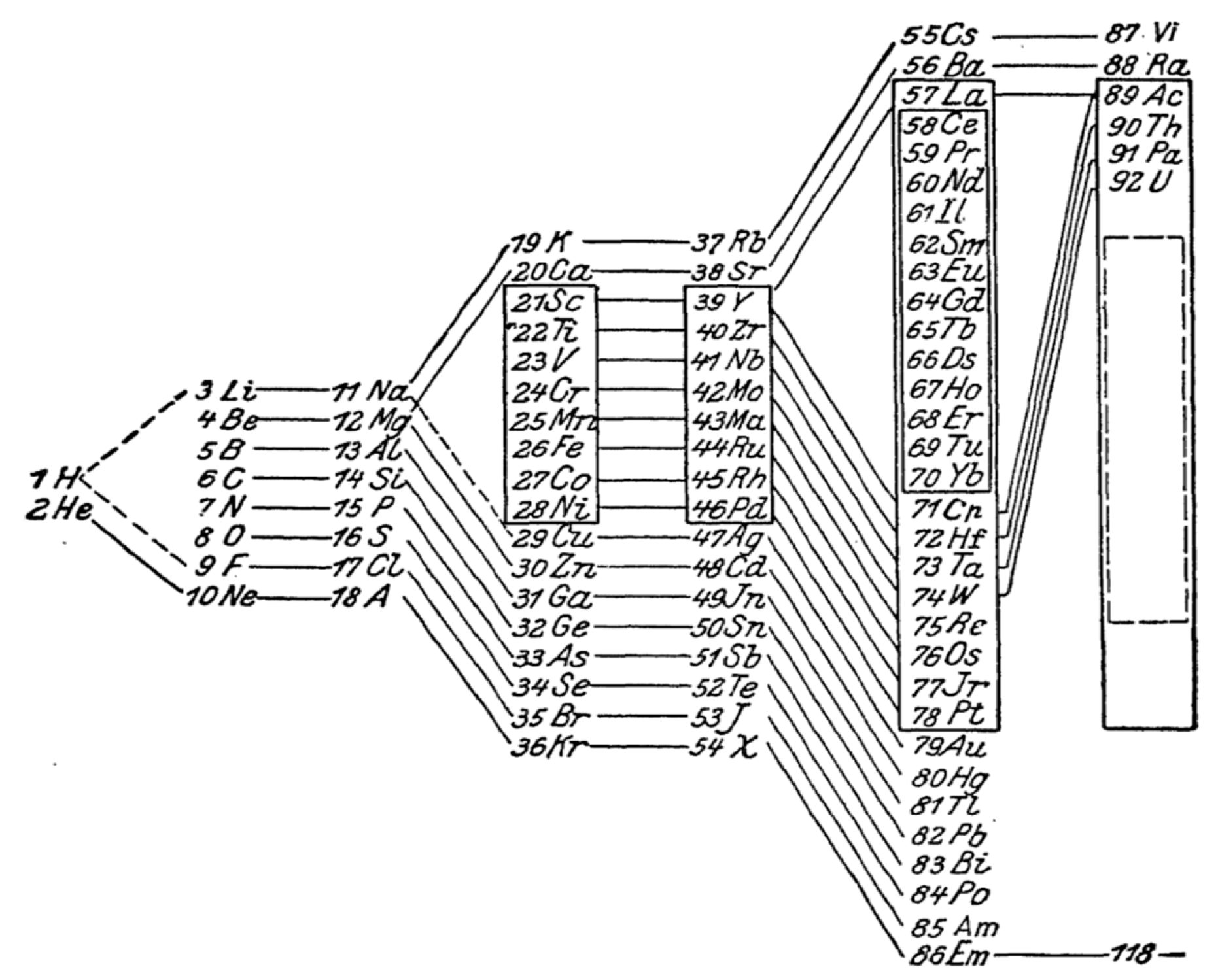
This figure shows a periodic system in relation to closed shells according to Max Born [13].
Figure 5.
This figure shows a periodic system in relation to closed shells according to Max Born [13].

Figure 6.
Nucleus cross section probability as a function of Atomic weight A.
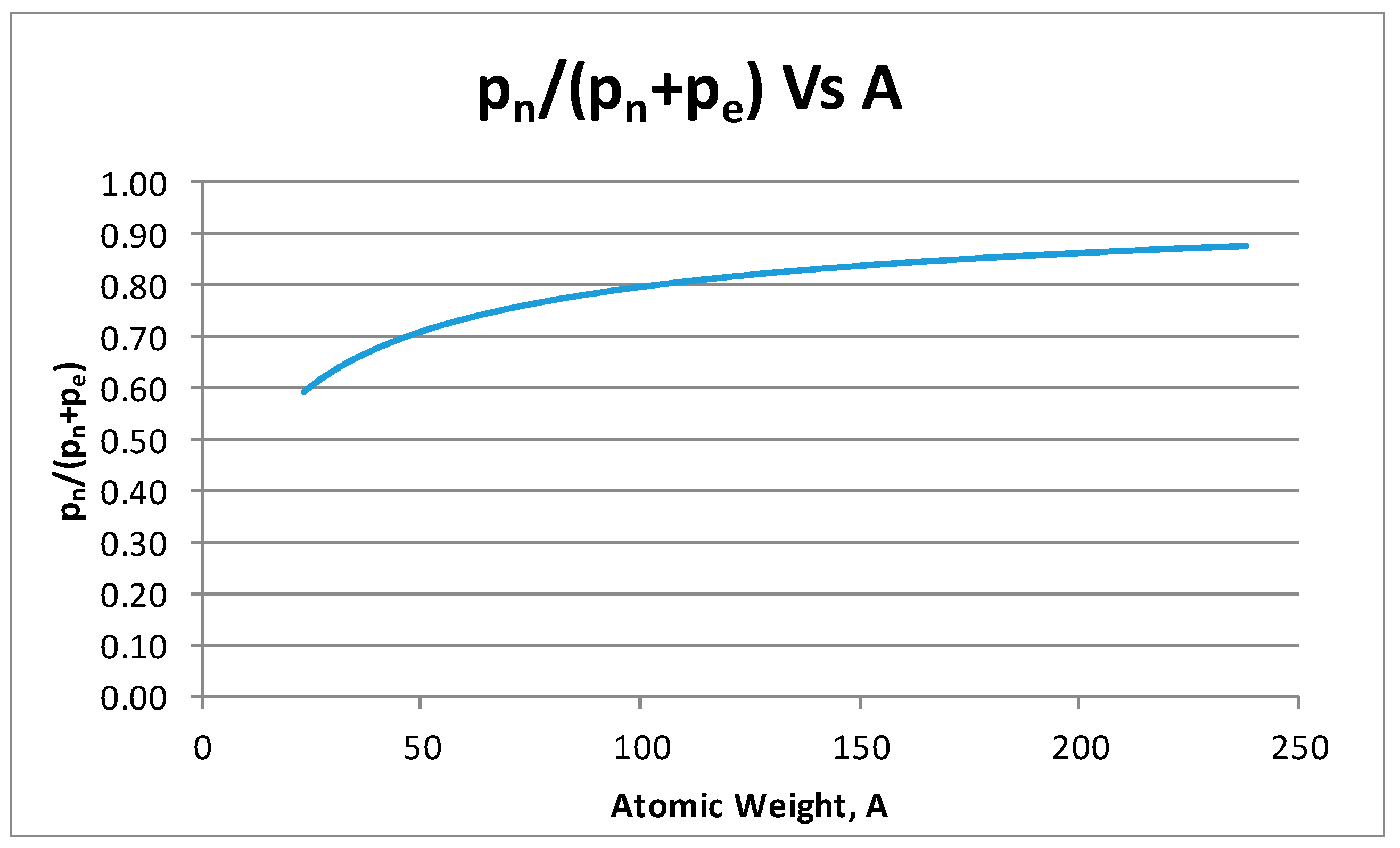
Figure 7.
We can see that the electron cross section as a function of atomic weight A.
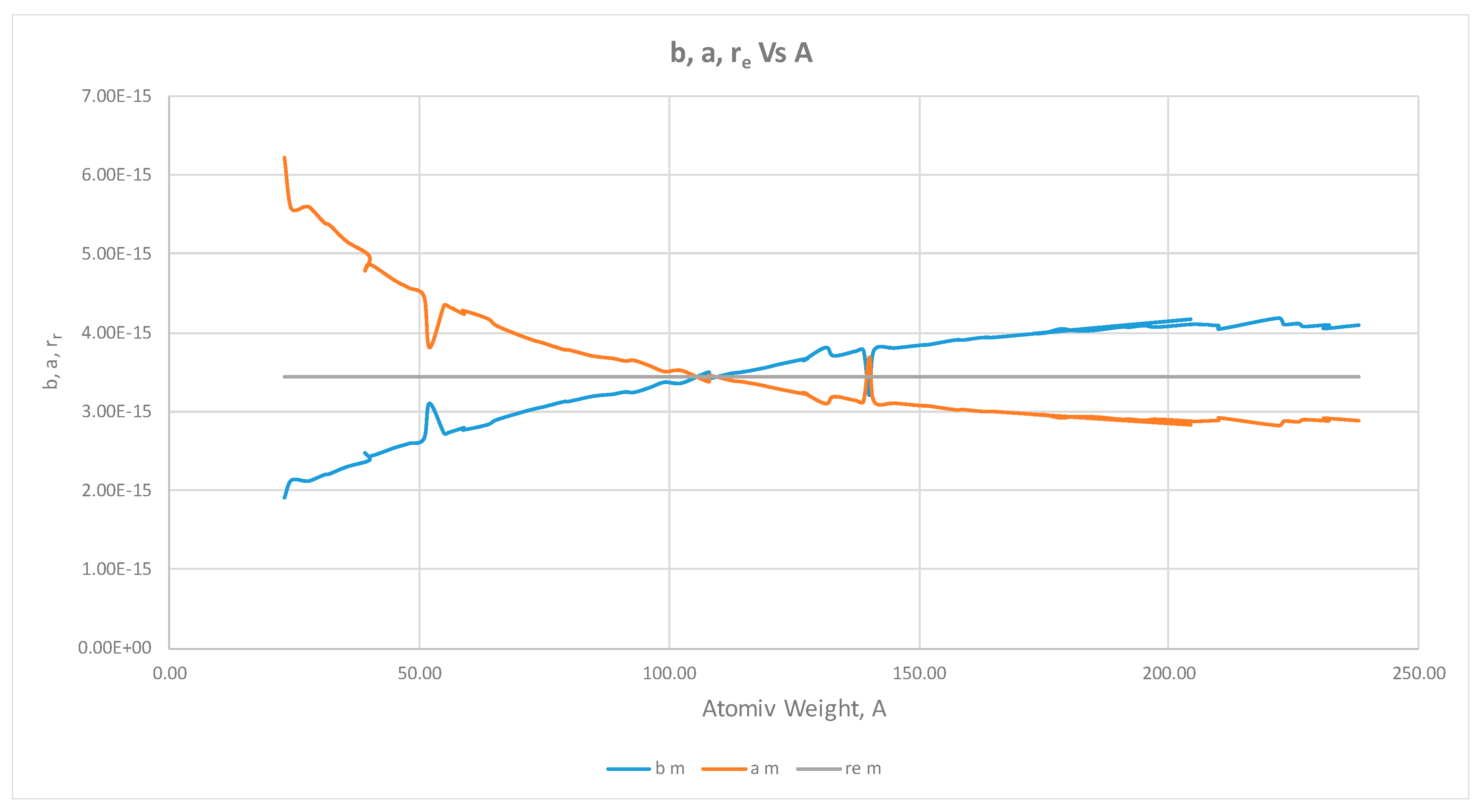
Figure 8.
The larger circle represents the minimum entropy radius. The intermediate circle represents the parameters of the wavelength according to D’ Broglie. The smaller circle represents the standard deviation of the uncertainty principle. Finally, the area of deformed ellipse of the cross section should have the same value of the minimum entropy radius πre2 = πai bi.

Figure 9.
Evolution plot of the effective resonance proton cross-section ellipse axis as a function of atomic weight A.
Figure 9.
Evolution plot of the effective resonance proton cross-section ellipse axis as a function of atomic weight A.

Figure 10.
Size of the electron as a function of the atomic weight A.
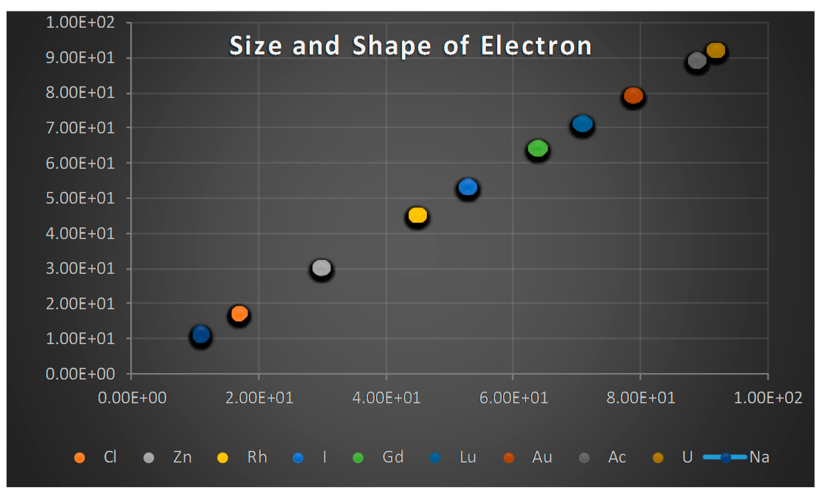
Figure 11.
Functional dependence between proton and electron radii.

Table 1.
The table shows the calculations for effective cross sections by using Equations (19), (33) and (34).
Table 1.
The table shows the calculations for effective cross sections by using Equations (19), (33) and (34).
| ra | rp | E2 = E1 = E | λe = h/p | b | a | re | a/b | λ = hc/E | p = (E2/c2 + 2mE)1/2 | υ = (E/mc2 + 1) | β = v/c | (pe/(pn + pe)) | (σ2 − σ1)((pn + pe)/pe) | b | σ2 | σ1 | σ2 | σ1 | (σ2 − σ1)/σ2 |
|---|---|---|---|---|---|---|---|---|---|---|---|---|---|---|---|---|---|---|---|
| m | m | MeV | m | m | m | m | m | Kg·m/s | m | m2 | m | cm2/gr | cm2/gr | cm2 | cm2 | % | |||
| 1.9 × 10⁻¹⁰ | 8.3 × 10⁻¹⁶ | 0.0010721 | 3.32187 × 10⁻¹⁶ | 7.4503 × 10⁻¹⁶ | 9.81203 × 10⁻¹⁶ | 2.67315 × 10⁻¹⁵ | 1.31699822 | 1.15802 × 10⁻⁹ | 1.99887 × 10⁻¹⁸ | 1.002098043 | 7.4503 × 10⁻¹⁶ | 0.38032585 | 5.91429 × 10⁻²³ | 7.4503 × 10⁻¹⁶ | 6435 | 542.9 | 2.45661 × 10⁻¹⁹ | 2.07257 × 10⁻²⁰ | 0.91563326 |
| 1.45 × 10⁻¹⁰ | 8.3 × 10⁻¹⁶ | 0.001305 | 3.01089 × 10⁻¹⁶ | 8.75431 × 10⁻¹⁶ | 8.35045 × 10⁻¹⁶ | 2.92396 × 10⁻¹⁵ | 0.95386719 | 9.51353 × 10⁻¹⁰ | 2.20533 × 10⁻¹⁸ | 1.002553816 | 8.75431 × 10⁻¹⁶ | 0.41438056 | 4.86109 × 10⁻²³ | 8.75431 × 10⁻¹⁶ | 5444 | 453 | 2.19717 × 10⁻¹⁹ | 1.82828 × 10⁻²⁰ | 0.91678913 |
| 1.431 × 10⁻¹⁰ | 8.3 × 10⁻¹⁶ | 0.0015596 | 2.75419 × 10⁻¹⁶ | 8.17537 × 10⁻¹⁶ | 8.94179 × 10⁻¹⁶ | 2.81511 × 10⁻¹⁵ | 1.0937471 | 7.96047 × 10⁻¹⁰ | 2.41087 × 10⁻¹⁸ | 1.003052055 | 8.17537 × 10⁻¹⁶ | 0.37957085 | 4.24312 × 10⁻²³ | 8.17537 × 10⁻¹⁶ | 3957 | 362.1 | 1.77279 × 10⁻¹⁹ | 1.62226 × 10⁻²⁰ | 0.90849128 |
| 1.11 × 10⁻¹⁰ | 8.3 × 10⁻¹⁶ | 0.00184 | 2.53566 × 10⁻¹⁶ | 8.00318 × 10⁻¹⁶ | 9.13418 × 10⁻¹⁶ | 2.78156 × 10⁻¹⁵ | 1.14131904 | 6.74737 × 10⁻¹⁰ | 2.61864 × 10⁻¹⁸ | 1.003600783 | 8.00318 × 10⁻¹⁶ | 0.36766952 | 3.65753 × 10⁻²³ | 8.00318 × 10⁻¹⁶ | 3190 | 309 | 1.48796 × 10⁻¹⁹ | 1.44132 × 10⁻²⁰ | 0.9031348 |
| 9.8 × 10⁻¹¹ | 8.3 × 10⁻¹⁶ | 0.00215 | 2.34575 × 10⁻¹⁶ | 8.0335 × 10⁻¹⁶ | 9.09971 × 10⁻¹⁶ | 2.7877 × 10⁻¹⁵ | 1.13272048 | 5.77449 × 10⁻¹⁰ | 2.83065 × 10⁻¹⁸ | 1.004207436 | 8.0335 × 10⁻¹⁶ | 0.35368271 | 3.23379 × 10⁻²³ | 8.0335 × 10⁻¹⁶ | 2470 | 249 | 1.27025 × 10⁻¹⁹ | 1.28053 × 10⁻²⁰ | 0.89919028 |
| 8.8 × 10⁻¹¹ | 8.3 × 10⁻¹⁶ | 0.00247 | 2.18853 × 10⁻¹⁶ | 7.96621 × 10⁻¹⁶ | 9.17658 × 10⁻¹⁶ | 2.77099 × 10⁻¹⁵ | 1.15193793 | 5.02638 × 10⁻¹⁰ | 3.034 × 10⁻¹⁸ | 1.004833659 | 7.96621 × 10⁻¹⁶ | 0.34568665 | 2.85404 × 10⁻²³ | 7.96621 × 10⁻¹⁶ | 2070 | 217 | 1.10214 × 10⁻¹⁹ | 1.15539 × 10⁻²⁰ | 0.89516908 |
| 7.1 × 10⁻¹¹ | 8.3 × 10⁻¹⁶ | 0.002822 | 2.04749 × 10⁻¹⁶ | 8.06047 × 10⁻¹⁶ | 9.06926 × 10⁻¹⁶ | 2.78582 × 10⁻¹⁵ | 1.12515151 | 4.39942 × 10⁻¹⁰ | 3.24299 × 10⁻¹⁸ | 1.005522505 | 8.06047 × 10⁻¹⁶ | 0.33306326 | 2.58065 × 10⁻²³ | 8.06047 × 10⁻¹⁶ | 1640 | 177 | 9.65487 × 10⁻²⁰ | 1.04202 × 10⁻²⁰ | 0.89207317 |
| 7.9 × 10⁻¹¹ | 8.3 × 10⁻¹⁶ | 0.0032029 | 1.92189 × 10⁻¹⁶ | 8.0681 × 10⁻¹⁶ | 9.06069 × 10⁻¹⁶ | 2.77356 × 10⁻¹⁵ | 1.12302669 | 3.87622 × 10⁻¹⁰ | 3.45493 × 10⁻¹⁸ | 1.006267906 | 8.0681 × 10⁻¹⁶ | 0.3368301 | 2.23054 × 10⁻²³ | 8.0681 × 10⁻¹⁶ | 1275 | 142.7 | 8.45775 × 10⁻²⁰ | 9.46604 × 10⁻²¹ | 0.88807843 |
| 2.43 × 10⁻¹⁰ | 8.3 × 10⁻¹⁶ | 0.0036074 | 1.81094 × 10⁻¹⁶ | 8.61142 × 10⁻¹⁶ | 8.48902 × 10⁻¹⁶ | 2.90268 × 10⁻¹⁵ | 0.98578609 | 3.44158 × 10⁻¹⁰ | 3.66661 × 10⁻¹⁸ | 1.007059491 | 8.61142 × 10⁻¹⁶ | 0.3368301 | 2.05867 × 10⁻²³ | 8.61142 × 10⁻¹⁶ | 1200 | 133 | 7.79125 × 10⁻²⁰ | 8.63531 × 10⁻²¹ | 0.88916667 |
| 1.94 × 10⁻¹⁰ | 8.3 × 10⁻¹⁶ | 0.0040381 | 1.71164 × 10⁻¹⁶ | 8.26435 × 10⁻¹⁶ | 8.84552 × 10⁻¹⁶ | 2.82948 × 10⁻¹⁵ | 1.070322 | 3.0745 × 10⁻¹⁰ | 3.87932 × 10⁻¹⁸ | 1.007902348 | 8.26435 × 10⁻¹⁶ | 0.32190293 | 1.87112 × 10⁻²³ | 8.26435 × 10⁻¹⁶ | 1023 | 118 | 6.80852 × 10⁻²⁰ | 7.85343 × 10⁻²¹ | 0.88465298 |
| 1.84 × 10⁻¹⁰ | 8.3 × 10⁻¹⁶ | 0.00449 | 1.62322 × 10⁻¹⁶ | 8.31531 × 10⁻¹⁶ | 8.79132 × 10⁻¹⁶ | 2.83979 × 10⁻¹⁵ | 1.05724525 | 2.76507 × 10⁻¹⁰ | 4.09063 × 10⁻¹⁸ | 1.008786693 | 8.31531 × 10⁻¹⁶ | 0.30696061 | 1.74654 × 10⁻²³ | 8.31531 × 10⁻¹⁶ | 815 | 96.9 | 6.08462 × 10⁻²⁰ | 7.23435 × 10⁻²¹ | 0.88110429 |
| 1.76 × 10⁻¹⁰ | 8.3 × 10⁻¹⁶ | 0.00497 | 1.54285 × 10⁻¹⁶ | 8.31466 × 10⁻¹⁶ | 8.792 × 10⁻¹⁶ | 2.83908 × 10⁻¹⁵ | 1.05741018 | 2.49802 × 10⁻¹⁰ | 4.30374 × 10⁻¹⁸ | 1.009726027 | 8.31466 × 10⁻¹⁶ | 0.29800529 | 1.61198 × 10⁻²³ | 8.31466 × 10⁻¹⁶ | 688 | 83.8 | 5.47006 × 10⁻²⁰ | 6.66266 × 10⁻²¹ | 0.87819767 |
| 1.71 × 10⁻¹⁰ | 8.3 × 10⁻¹⁶ | 0.0054651 | 1.4713 × 10⁻¹⁶ | 8.36832 × 10⁻¹⁶ | 8.73562 × 10⁻¹⁶ | 2.85004 × 10⁻¹⁵ | 1.04389139 | 2.27172 × 10⁻¹⁰ | 4.51301 × 10⁻¹⁸ | 1.010694912 | 8.36832 × 10⁻¹⁶ | 0.29102595 | 1.49463 × 10⁻²³ | 8.36832 × 10⁻¹⁶ | 587 | 72.77 | 4.96531 × 10⁻²⁰ | 6.15546 × 10⁻²¹ | 0.87603066 |
| 1.66 × 10⁻¹⁰ | 8.3 × 10⁻¹⁶ | 0.0059892 | 1.40545 × 10⁻¹⁶ | 1.06767 × 10⁻¹⁵ | 6.84695 × 10⁻¹⁶ | 3.30564 × 10⁻¹⁵ | 0.64130057 | 2.07292 × 10⁻¹⁰ | 4.72446 × 10⁻¹⁸ | 1.011720548 | 1.06767 × 10⁻¹⁵ | 0.35264878 | 1.30228 × 10⁻²³ | 1.06767 × 10⁻¹⁵ | 597.7 | 65.74 | 5.16003 × 10⁻²⁰ | 5.67543 × 10⁻²¹ | 0.89001171 |
| 1.61 × 10⁻¹⁰ | 8.3 × 10⁻¹⁶ | 0.00654 | 1.34497 × 10⁻¹⁶ | 8.35959 × 10⁻¹⁶ | 8.74475 × 10⁻¹⁶ | 2.84669 × 10⁻¹⁵ | 1.04607322 | 1.89834 × 10⁻¹⁰ | 4.93692 × 10⁻¹⁸ | 1.012798434 | 8.35959 × 10⁻¹⁶ | 0.28026267 | 1.28253 × 10⁻²³ | 8.35959 × 10⁻¹⁶ | 452 | 58 | 4.1236 × 10⁻²⁰ | 5.29134 × 10⁻²¹ | 0.87168142 |
| 1.558 × 10⁻¹⁰ | 8.3 × 10⁻¹⁶ | 0.00711 | 1.28993 × 10⁻¹⁶ | 8.32631 × 10⁻¹⁶ | 8.7797 × 10⁻¹⁶ | 2.83848 × 10⁻¹⁵ | 1.054452 | 1.74615 × 10⁻¹⁰ | 5.14757 × 10⁻¹⁸ | 1.013913894 | 8.32631 × 10⁻¹⁶ | 0.27690045 | 1.18832 × 10⁻²³ | 8.32631 × 10⁻¹⁶ | 408 | 53.2 | 3.78384 × 10⁻²⁰ | 4.93383 × 10⁻²¹ | 0.86960784 |
| 1.52 × 10⁻¹⁰ | 8.3 × 10⁻¹⁶ | 0.00771 | 1.23872 × 10⁻¹⁶ | 8.37916 × 10⁻¹⁶ | 8.72432 × 10⁻¹⁶ | 2.84929 × 10⁻¹⁵ | 1.04119234 | 1.61027 × 10⁻¹⁰ | 5.36037 × 10⁻¹⁸ | 1.015088063 | 8.37916 × 10⁻¹⁶ | 0.27129321 | 1.1142 × 10⁻²³ | 8.37916 × 10⁻¹⁶ | 356 | 47.1 | 3.48366 × 10⁻²⁰ | 4.609 × 10⁻²¹ | 0.86769663 |
| 1.49 × 10⁻¹⁰ | 8.3 × 10⁻¹⁶ | 0.00833 | 1.19173 × 10⁻¹⁶ | 8.2619 × 10⁻¹⁶ | 8.84815 × 10⁻¹⁶ | 2.82221 × 10⁻¹⁵ | 1.07095852 | 1.49041 × 10⁻¹⁰ | 5.57173 × 10⁻¹⁸ | 1.01630137 | 8.2619 × 10⁻¹⁶ | 0.2680679 | 1.03504 × 10⁻²³ | 8.2619 × 10⁻¹⁶ | 329 | 44.3 | 3.20634 × 10⁻²⁰ | 4.31735 × 10⁻²¹ | 0.86534954 |
| 1.45 × 10⁻¹⁰ | 8.3 × 10⁻¹⁶ | 0.0089789 | 1.14786 × 10⁻¹⁶ | 8.20536 × 10⁻¹⁶ | 8.90912 × 10⁻¹⁶ | 2.81146 × 10⁻¹⁵ | 1.08576779 | 1.3827 × 10⁻¹⁰ | 5.78468 × 10⁻¹⁸ | 1.017571233 | 8.20536 × 10⁻¹⁶ | 0.25633201 | 9.88449 × 10⁻²⁴ | 8.20536 × 10⁻¹⁶ | 278 | 38.3 | 2.93366 × 10⁻²⁰ | 4.0417 × 10⁻²¹ | 0.86223022 |
| 1.42 × 10⁻¹⁰ | 8.3 × 10⁻¹⁶ | 0.00966 | 1.10665 × 10⁻¹⁶ | 8.38682 × 10⁻¹⁶ | 8.71635 × 10⁻¹⁶ | 2.84463 × 10⁻¹⁵ | 1.03929089 | 1.28521 × 10⁻¹⁰ | 6.00007 × 10⁻¹⁸ | 1.01890411 | 8.38682 × 10⁻¹⁶ | 0.25714096 | 9.22926 × 10⁻²⁴ | 8.38682 × 10⁻¹⁶ | 254 | 35.1 | 2.7588 × 10⁻²⁰ | 3.81236 × 10⁻²¹ | 0.86181102 |
| 1.35 × 10⁻¹⁰ | 8.3 × 10⁻¹⁶ | 0.0103671 | 1.06825 × 10⁻¹⁶ | 8.44395 × 10⁻¹⁶ | 8.65739 × 10⁻¹⁶ | 2.86404 × 10⁻¹⁵ | 1.02527748 | 1.19755 × 10⁻¹⁰ | 6.21579 × 10⁻¹⁸ | 1.020287867 | 8.44395 × 10⁻¹⁶ | 0.25164879 | 8.75949 × 10⁻²⁴ | 8.44395 × 10⁻¹⁶ | 221 | 31 | 2.55858 × 10⁻²⁰ | 3.58896 × 10⁻²¹ | 0.85972851 |
| 1.52 × 10⁻¹⁰ | 8.3 × 10⁻¹⁶ | 0.0111 | 1.03238 × 10⁻¹⁶ | 8.49084 × 10⁻¹⁶ | 8.60957 × 10⁻¹⁶ | 2.87074 × 10⁻¹⁵ | 1.01398278 | 1.11848 × 10⁻¹⁰ | 6.43175 × 10⁻¹⁸ | 1.021722114 | 8.49084 × 10⁻¹⁶ | 0.24740235 | 8.28839 × 10⁻²⁴ | 8.49084 × 10⁻¹⁶ | 198 | 28.1 | 2.38831 × 10⁻²⁰ | 3.38947 × 10⁻²¹ | 0.85808081 |
| 1.14 × 10⁻¹⁰ | 8.3 × 10⁻¹⁶ | 0.0118667 | 9.98471 × 10⁻¹⁷ | 8.49827 × 10⁻¹⁶ | 8.60205 × 10⁻¹⁶ | 2.87015 × 10⁻¹⁵ | 1.01221185 | 1.04622 × 10⁻¹⁰ | 6.65017 × 10⁻¹⁸ | 1.023222505 | 8.49827 × 10⁻¹⁶ | 0.24351097 | 7.83861 × 10⁻²⁴ | 8.49827 × 10⁻¹⁶ | 179.2 | 25.77 | 2.22939 × 10⁻²⁰ | 3.20599 × 10⁻²¹ | 0.8561942 |
| 1.03 × 10⁻¹⁰ | 8.3 × 10⁻¹⁶ | 0.0126578 | 9.66766 × 10⁻¹⁷ | 8.54015 × 10⁻¹⁶ | 8.55986 × 10⁻¹⁶ | 2.87873 × 10⁻¹⁵ | 1.00230776 | 9.8083 × 10⁻¹¹ | 6.86826 × 10⁻¹⁸ | 1.024770646 | 8.54015 × 10⁻¹⁶ | 0.23819988 | 7.47066 × 10⁻²⁴ | 8.54015 × 10⁻¹⁶ | 158.9 | 23.18 | 2.08344 × 10⁻²⁰ | 3.03927 × 10⁻²¹ | 0.85412209 |
| 1.35 × 10⁻¹⁰ | 8.3 × 10⁻¹⁶ | 0.0134737 | 9.37038 × 10⁻¹⁷ | 8.49723 × 10⁻¹⁶ | 8.6031 × 10⁻¹⁶ | 2.8675 × 10⁻¹⁵ | 1.01245862 | 9.21436 × 10⁻¹¹ | 7.08616 × 10⁻¹⁸ | 1.026367319 | 8.49723 × 10⁻¹⁶ | 0.23536126 | 7.06563 × 10⁻²⁴ | 8.49723 × 10⁻¹⁶ | 147.1 | 21.76 | 1.95168 × 10⁻²⁰ | 2.88706 × 10⁻²¹ | 0.85207342 |
| 1.9 × 10⁻¹⁰ | 8.3 × 10⁻¹⁶ | 0.0143256 | 9.08749 × 10⁻¹⁷ | 8.51054 × 10⁻¹⁶ | 8.58964 × 10⁻¹⁶ | 2.86937 × 10⁻¹⁵ | 1.00929502 | 8.66641 × 10⁻¹¹ | 7.30674 × 10⁻¹⁸ | 1.028034442 | 8.51054 × 10⁻¹⁶ | 0.22992348 | 6.7536 × 10⁻²⁴ | 8.51054 × 10⁻¹⁶ | 131.3 | 19.71 | 1.82708 × 10⁻²⁰ | 2.74271 × 10⁻²¹ | 0.84988576 |
| 2.65 × 10⁻¹⁰ | 8.3 × 10⁻¹⁶ | 0.015199 | 8.82253 × 10⁻¹⁷ | 8.48897 × 10⁻¹⁶ | 8.61147 × 10⁻¹⁶ | 2.86291 × 10⁻¹⁵ | 1.01443044 | 8.1684 × 10⁻¹¹ | 7.52619 × 10⁻¹⁸ | 1.02974364 | 8.48897 × 10⁻¹⁶ | 0.22681006 | 6.42019 × 10⁻²⁴ | 8.48897 × 10⁻¹⁶ | 121 | 18.4 | 1.71731 × 10⁻²⁰ | 2.61145 × 10⁻²¹ | 0.84793388 |
| 2.19 × 10⁻¹⁰ | 8.3 × 10⁻¹⁶ | 0.0161046 | 8.57088 × 10⁻¹⁷ | 8.43835 × 10⁻¹⁶ | 8.66313 × 10⁻¹⁶ | 2.84958 × 10⁻¹⁵ | 1.0266387 | 7.70907 × 10⁻¹¹ | 7.74716 × 10⁻¹⁸ | 1.031515851 | 8.43835 × 10⁻¹⁶ | 0.22230144 | 6.13006 × 10⁻²⁴ | 8.43835 × 10⁻¹⁶ | 110.8 | 17.14 | 1.6121 × 10⁻²⁰ | 2.49381 × 10⁻²¹ | 0.84530686 |
| 2.12 × 10⁻¹⁰ | 8.3 × 10⁻¹⁶ | 0.0170384 | 8.33271 × 10⁻¹⁷ | 8.40366 × 10⁻¹⁶ | 8.69888 × 10⁻¹⁶ | 2.83978 × 10⁻¹⁵ | 1.03513002 | 7.28657 × 10⁻¹¹ | 7.9686 × 10⁻¹⁸ | 1.033343249 | 8.40366 × 10⁻¹⁶ | 0.21943832 | 5.83858 × 10⁻²⁴ | 8.40366 × 10⁻¹⁶ | 102.9 | 16.12 | 1.5192 × 10⁻²⁰ | 2.37993 × 10⁻²¹ | 0.84334305 |
| 2.06 × 10⁻¹⁰ | 8.3 × 10⁻¹⁶ | 0.017997 | 8.10775 × 10⁻¹⁷ | 8.40175 × 10⁻¹⁶ | 8.70087 × 10⁻¹⁶ | 2.83762 × 10⁻¹⁵ | 1.03560254 | 6.89846 × 10⁻¹¹ | 8.18969 × 10⁻¹⁸ | 1.035219178 | 8.40175 × 10⁻¹⁶ | 0.21626625 | 5.58225 × 10⁻²⁴ | 8.40175 × 10⁻¹⁶ | 94.7 | 15 | 1.43446 × 10⁻²⁰ | 2.27212 × 10⁻²¹ | 0.84160507 |
| 1.98 × 10⁻¹⁰ | 8.3 × 10⁻¹⁶ | 0.0189856 | 7.89384 × 10⁻¹⁷ | 8.3501 × 10⁻¹⁶ | 8.75469 × 10⁻¹⁶ | 2.81176 × 10⁻¹⁵ | 1.04845334 | 6.53925 × 10⁻¹¹ | 8.41162 × 10⁻¹⁸ | 1.037153816 | 8.3501 × 10⁻¹⁶ | 0.21113252 | 5.35698 × 10⁻²⁴ | 8.3501 × 10⁻¹⁶ | 87.84 | 14.09 | 1.3552 × 10⁻²⁰ | 2.17382 × 10⁻²¹ | 0.83959472 |
| 1.9 × 10⁻¹⁰ | 8.3 × 10⁻¹⁶ | 0.019999 | 7.69124 × 10⁻¹⁷ | 8.38586 × 10⁻¹⁶ | 8.71735 × 10⁻¹⁶ | 2.82877 × 10⁻¹⁵ | 1.03952958 | 6.20789 × 10⁻¹¹ | 8.6332 × 10⁻¹⁸ | 1.039136986 | 8.38586 × 10⁻¹⁶ | 0.20958319 | 5.12713 × 10⁻²⁴ | 8.38586 × 10⁻¹⁶ | 80.6 | 13.1 | 1.28406 × 10⁻²⁰ | 2.08699 × 10⁻²¹ | 0.83746898 |
| 1.83 × 10⁻¹⁰ | 8.3 × 10⁻¹⁶ | 0.021044 | 7.49784 × 10⁻¹⁷ | 8.51277 × 10⁻¹⁶ | 8.58739 × 10⁻¹⁶ | 2.85851 × 10⁻¹⁵ | 1.00876587 | 5.89962 × 10⁻¹¹ | 8.85588 × 10⁻¹⁸ | 1.041181996 | 8.51277 × 10⁻¹⁶ | 0.20968537 | 4.89693 × 10⁻²⁴ | 8.51277 × 10⁻¹⁶ | 74.81 | 12.29 | 1.22866 × 10⁻²⁰ | 2.01848 × 10⁻²¹ | 0.83571715 |
| 2.65 × 10⁻¹⁰ | 8.3 × 10⁻¹⁶ | 0.0221 | 7.31652 × 10⁻¹⁷ | 8.38045 × 10⁻¹⁶ | 8.72298 × 10⁻¹⁶ | 2.8237 × 10⁻¹⁵ | 1.04087264 | 5.61772 × 10⁻¹¹ | 9.07536 × 10⁻¹⁸ | 1.043248532 | 8.38045 × 10⁻¹⁶ | 0.20330645 | 4.73511 × 10⁻²⁴ | 8.38045 × 10⁻¹⁶ | 68.8 | 11.4 | 1.15468 × 10⁻²⁰ | 1.91327 × 10⁻²¹ | 0.83430233 |
| 1.34 × 10⁻¹⁰ | 8.3 × 10⁻¹⁶ | 0.0232 | 7.14096 × 10⁻¹⁷ | 8.33355 × 10⁻¹⁶ | 8.77207 × 10⁻¹⁶ | 2.81177 × 10⁻¹⁵ | 1.05262153 | 5.35136 × 10⁻¹¹ | 9.29847 × 10⁻¹⁸ | 1.045401174 | 8.33355 × 10⁻¹⁶ | 0.20000646 | 4.55397 × 10⁻²⁴ | 8.33355 × 10⁻¹⁶ | 64.1 | 10.8 | 1.09538 × 10⁻²⁰ | 1.84557 × 10⁻²¹ | 0.83151326 |
| 1.69 × 10⁻¹⁰ | 8.3 × 10⁻¹⁶ | 0.0244 | 6.96315 × 10⁻¹⁷ | 8.60007 × 10⁻¹⁶ | 8.50022 × 10⁻¹⁶ | 2.87351 × 10⁻¹⁵ | 0.98838955 | 5.08818 × 10⁻¹¹ | 9.53592 × 10⁻¹⁸ | 1.047749511 | 8.60007 × 10⁻¹⁶ | 0.20194504 | 4.34616 × 10⁻²⁴ | 8.60007 × 10⁻¹⁶ | 59 | 10 | 1.05681 × 10⁻²⁰ | 1.7912 × 10⁻²¹ | 0.83050847 |
| 1.65 × 10⁻¹⁰ | 8.3 × 10⁻¹⁶ | 0.025514 | 6.80944 × 10⁻¹⁷ | 8.33019 × 10⁻¹⁶ | 8.77561 × 10⁻¹⁶ | 2.80655 × 10⁻¹⁵ | 1.05346946 | 4.86602 × 10⁻¹¹ | 9.75117 × 10⁻¹⁸ | 1.04992955 | 8.33019 × 10⁻¹⁶ | 0.19442131 | 4.22078 × 10⁻²⁴ | 8.33019 × 10⁻¹⁶ | 55.39 | 9.59 | 9.92435 × 10⁻²¹ | 1.71826 × 10⁻²¹ | 0.82686405 |
| 1.61 × 10⁻¹⁰ | 8.3 × 10⁻¹⁶ | 0.0267 | 6.65648 × 10⁻¹⁷ | 8.3772 × 10⁻¹⁶ | 8.72636 × 10⁻¹⁶ | 2.8157 × 10⁻¹⁵ | 1.04168041 | 4.64987 × 10⁻¹¹ | 9.97523 × 10⁻¹⁸ | 1.052250489 | 8.3772 × 10⁻¹⁶ | 0.19118457 | 4.08514 × 10⁻²⁴ | 8.3772 × 10⁻¹⁶ | 50.65 | 8.809 | 9.45448 × 10⁻²¹ | 1.64431 × 10⁻²¹ | 0.82608095 |
| 1.56 × 10⁻¹⁰ | 8.3 × 10⁻¹⁶ | 0.0279 | 6.51176 × 10⁻¹⁷ | 8.3565 × 10⁻¹⁶ | 8.74799 × 10⁻¹⁶ | 2.80837 × 10⁻¹⁵ | 1.04684853 | 4.44988 × 10⁻¹¹ | 1.01969 × 10⁻¹⁷ | 1.054598826 | 8.3565 × 10⁻¹⁶ | 0.18822821 | 3.94774 × 10⁻²⁴ | 8.3565 × 10⁻¹⁶ | 47.3 | 8.32 | 9.0168 × 10⁻²¹ | 1.58604 × 10⁻²¹ | 0.82410148 |
| 1.45 × 10⁻¹⁰ | 8.3 × 10⁻¹⁶ | 0.0292001 | 6.36515 × 10⁻¹⁷ | 8.37622 × 10⁻¹⁶ | 8.72738 × 10⁻¹⁶ | 2.81069 × 10⁻¹⁵ | 1.04192371 | 4.25175 × 10⁻¹¹ | 1.04318 × 10⁻¹⁷ | 1.057143053 | 8.37622 × 10⁻¹⁶ | 0.18508991 | 3.817 × 10⁻²⁴ | 8.37622 × 10⁻¹⁶ | 43.6 | 7.76 | 8.59455 × 10⁻²¹ | 1.52967 × 10⁻²¹ | 0.82201835 |
| 1.33 × 10⁻¹⁰ | 8.3 × 10⁻¹⁶ | 0.030491 | 6.22895 × 10⁻¹⁷ | 8.42372 × 10⁻¹⁶ | 8.67817 × 10⁻¹⁶ | 2.81987 × 10⁻¹⁵ | 1.030206 | 4.07174 × 10⁻¹¹ | 1.06599 × 10⁻¹⁷ | 1.059669276 | 8.42372 × 10⁻¹⁶ | 0.18349443 | 3.68367 × 10⁻²⁴ | 8.42372 × 10⁻¹⁶ | 40.73 | 7.31 | 8.2378 × 10⁻²¹ | 1.47848 × 10⁻²¹ | 0.82052541 |
| 1.23 × 10⁻¹⁰ | 8.3 × 10⁻¹⁶ | 0.0318 | 6.0994 × 10⁻¹⁷ | 8.4856 × 10⁻¹⁶ | 8.61489 × 10⁻¹⁶ | 2.8326 × 10⁻¹⁵ | 1.01523657 | 3.90414 × 10⁻¹¹ | 1.08863 × 10⁻¹⁷ | 1.06223092 | 8.4856 × 10⁻¹⁶ | 0.18022094 | 3.58117 × 10⁻²⁴ | 8.4856 × 10⁻¹⁶ | 37.2 | 6.74 | 7.88212 × 10⁻²¹ | 1.4281 × 10⁻²¹ | 0.8188172 |
| 1.15 × 10⁻¹⁰ | 8.3 × 10⁻¹⁶ | 0.0331694 | 5.97216 × 10⁻¹⁷ | 8.4295 × 10⁻¹⁶ | 8.67222 × 10⁻¹⁶ | 2.81478 × 10⁻¹⁵ | 1.02879346 | 3.74295 × 10⁻¹¹ | 1.11182 × 10⁻¹⁷ | 1.064910763 | 8.4295 × 10⁻¹⁶ | 0.17890145 | 3.44527 × 10⁻²⁴ | 8.4295 × 10⁻¹⁶ | 35.82 | 6.55 | 7.54808 × 10⁻²¹ | 1.38023 × 10⁻²¹ | 0.81714126 |
| 1.08 × 10⁻¹⁰ | 8.3 × 10⁻¹⁶ | 0.0356 | 5.76468 × 10⁻¹⁷ | 8.81889 × 10⁻¹⁶ | 8.28931 × 10⁻¹⁶ | 2.90333 × 10⁻¹⁵ | 0.93994974 | 3.4874 × 10⁻¹¹ | 1.15184 × 10⁻¹⁷ | 1.069667319 | 8.81889 × 10⁻¹⁶ | 0.18473575 | 3.19014 × 10⁻²⁴ | 8.81889 × 10⁻¹⁶ | 33.2 | 6.13 | 7.23856 × 10⁻²¹ | 1.33652 × 10⁻²¹ | 0.81536145 |
| 2.98 × 10⁻¹⁰ | 8.3 × 10⁻¹⁶ | 0.0359 | 5.74055 × 10⁻¹⁷ | 8.41564 × 10⁻¹⁶ | 8.68651 × 10⁻¹⁶ | 2.80999 × 10⁻¹⁵ | 1.03218615 | 3.45826 × 10⁻¹¹ | 1.15668 × 10⁻¹⁷ | 1.070254403 | 8.41564 × 10⁻¹⁶ | 0.17393222 | 3.24433 × 10⁻²⁴ | 8.41564 × 10⁻¹⁶ | 31.4 | 5.86 | 6.92953 × 10⁻²¹ | 1.29322 × 10⁻²¹ | 0.8133758 |
| 2.53 × 10⁻¹⁰ | 8.3 × 10⁻¹⁶ | 0.0374 | 5.62425 × 10⁻¹⁷ | 8.47454 × 10⁻¹⁶ | 8.62614 × 10⁻¹⁶ | 2.81925 × 10⁻¹⁵ | 1.01788892 | 3.31956 × 10⁻¹¹ | 1.1806 × 10⁻¹⁷ | 1.073189824 | 8.47454 × 10⁻¹⁶ | 0.17176851 | 3.14575 × 10⁻²⁴ | 8.47454 × 10⁻¹⁶ | 29.2 | 5.5 | 6.65737 × 10⁻²¹ | 1.25396 × 10⁻²¹ | 0.81164384 |
| 1.95 × 10⁻¹⁰ | 8.3 × 10⁻¹⁶ | 0.0389 | 5.51475 × 10⁻¹⁷ | 8.45215 × 10⁻¹⁶ | 8.64899 × 10⁻¹⁶ | 2.81083 × 10⁻¹⁵ | 1.0232885 | 3.19156 × 10⁻¹¹ | 1.20404 × 10⁻¹⁷ | 1.076125245 | 8.45215 × 10⁻¹⁶ | 0.16982759 | 3.0463 × 10⁻²⁴ | 8.45215 × 10⁻¹⁶ | 27.7 | 5.27 | 6.38898 × 10⁻²¹ | 1.21552 × 10⁻²¹ | 0.80974729 |
| 2.98 × 10⁻¹⁰ | 8.3 × 10⁻¹⁶ | 0.03598 | 5.40873 × 10⁻¹⁷ | 6.0614 × 10⁻¹⁶ | 1.20603 × 10⁻¹⁵ | 2.37693 × 10⁻¹⁵ | 1.98969344 | 3.07002 × 10⁻¹¹ | 1.22765 × 10⁻¹⁷ | 1.079138943 | 6.0614 × 10⁻¹⁶ | 0.12698018 | 3.31246 × 10⁻²⁴ | 6.0614 × 10⁻¹⁶ | 26.35 | 8.27 | 6.13011 × 10⁻²¹ | 1.92395 × 10⁻²¹ | 0.68614801 |
| 2.47 × 10⁻¹⁰ | 8.3 × 10⁻¹⁶ | 0.0419906 | 5.30792 × 10⁻¹⁷ | 8.37273 × 10⁻¹⁶ | 8.73102 × 10⁻¹⁶ | 2.78515 × 10⁻¹⁵ | 1.04279179 | 2.95665 × 10⁻¹¹ | 1.25096 × 10⁻¹⁷ | 1.082173386 | 8.37273 × 10⁻¹⁶ | 0.16593206 | 2.86096 × 10⁻²⁴ | 8.37273 × 10⁻¹⁶ | 25.18 | 4.89 | 5.89137 × 10⁻²¹ | 1.14411 × 10⁻²¹ | 0.80579825 |
| 2.06 × 10⁻¹⁰ | 8.3 × 10⁻¹⁶ | 0.0436 | 5.20904 × 10⁻¹⁷ | 8.41025 × 10⁻¹⁶ | 8.69207 × 10⁻¹⁶ | 2.79139 × 10⁻¹⁵ | 1.03350884 | 2.84751 × 10⁻¹¹ | 1.27471 × 10⁻¹⁷ | 1.085322896 | 8.41025 × 10⁻¹⁶ | 0.16439518 | 2.77696 × 10⁻²⁴ | 8.41025 × 10⁻¹⁶ | 23.7 | 4.64 | 5.67654 × 10⁻²¹ | 1.11136 × 10⁻²¹ | 0.80421941 |
| 2.05 × 10⁻¹⁰ | 8.3 × 10⁻¹⁶ | 0.0452 | 5.11601 × 10⁻¹⁷ | 8.37123 × 10⁻¹⁶ | 8.73259 × 10⁻¹⁶ | 2.77858 × 10⁻¹⁵ | 1.04316772 | 2.74672 × 10⁻¹¹ | 1.29789 × 10⁻¹⁷ | 1.088454012 | 8.37123 × 10⁻¹⁶ | 0.16265799 | 2.69558 × 10⁻²⁴ | 8.37123 × 10⁻¹⁶ | 22.7 | 4.49 | 5.46567 × 10⁻²¹ | 1.08109 × 10⁻²¹ | 0.80220264 |
| 2.59 × 10⁻¹⁰ | 8.3 × 10⁻¹⁶ | 0.0468 | 5.0278 × 10⁻¹⁷ | 8.34624 × 10⁻¹⁶ | 8.75874 × 10⁻¹⁶ | 2.76908 × 10⁻¹⁵ | 1.04942362 | 2.65281 × 10⁻¹¹ | 1.32066 × 10⁻¹⁷ | 1.091585127 | 8.34624 × 10⁻¹⁶ | 0.15847319 | 2.64531 × 10⁻²⁴ | 8.34624 × 10⁻¹⁶ | 21 | 4.21 | 5.24326 × 10⁻²¹ | 1.05115 × 10⁻²¹ | 0.79952381 |
| 2.31 × 10⁻¹⁰ | 8.3 × 10⁻¹⁶ | 0.0485 | 4.93889 × 10⁻¹⁷ | 8.3229 × 10⁻¹⁶ | 8.78329 × 10⁻¹⁶ | 2.75992 × 10⁻¹⁵ | 1.05531588 | 2.55983 × 10⁻¹¹ | 1.34443 × 10⁻¹⁷ | 1.094911937 | 8.3229 × 10⁻¹⁶ | 0.15663383 | 2.57166 × 10⁻²⁴ | 8.3229 × 10⁻¹⁶ | 20.01 | 4.051 | 5.05057 × 10⁻²¹ | 1.02248 × 10⁻²¹ | 0.79755122 |
| 2.33 × 10⁻¹⁰ | 8.3 × 10⁻¹⁶ | 0.05023 | 4.8531 × 10⁻¹⁷ | 8.47317 × 10⁻¹⁶ | 8.62752 × 10⁻¹⁶ | 2.76591 × 10⁻¹⁵ | 1.0182166 | 2.47166 × 10⁻¹¹ | 1.3682 × 10⁻¹⁷ | 1.098297456 | 8.47317 × 10⁻¹⁶ | 0.15420304 | 2.51204 × 10⁻²⁴ | 8.47317 × 10⁻¹⁶ | 18.84 | 3.81 | 4.92106 × 10⁻²¹ | 9.95183 × 10⁻²² | 0.7977707 |
| 1.75 × 10⁻¹⁰ | 8.3 × 10⁻¹⁶ | 0.0519957 | 4.76998 × 10⁻¹⁷ | 8.317 × 10⁻¹⁶ | 8.78953 × 10⁻¹⁶ | 2.75151 × 10⁻¹⁵ | 1.05681514 | 2.38773 × 10⁻¹¹ | 1.39204 × 10⁻¹⁷ | 1.101752838 | 8.317 × 10⁻¹⁶ | 0.15197547 | 2.44769 × 10⁻²⁴ | 8.317 × 10⁻¹⁶ | 17.77 | 3.672 | 4.68879 × 10⁻²¹ | 9.68893 × 10⁻²² | 0.79335959 |
| 1.77 × 10⁻¹⁰ | 8.3 × 10⁻¹⁶ | 0.0537885 | 4.68982 × 10⁻¹⁷ | 8.31532 × 10⁻¹⁶ | 8.7913 × 10⁻¹⁶ | 2.74753 × 10⁻¹⁵ | 1.05724194 | 2.30814 × 10⁻¹¹ | 1.41583 × 10⁻¹⁷ | 1.105261252 | 8.31532 × 10⁻¹⁶ | 0.14969171 | 2.39028 × 10⁻²⁴ | 8.31532 × 10⁻¹⁶ | 16.76 | 3.5 | 4.52248 × 10⁻²¹ | 9.44432 × 10⁻²² | 0.79116945 |
| 2.47 × 10⁻¹⁰ | 8.3 × 10⁻¹⁶ | 0.0556 | 4.61278 × 10⁻¹⁷ | 8.26411 × 10⁻¹⁶ | 8.84578 × 10⁻¹⁶ | 2.73095 × 10⁻¹⁵ | 1.07038524 | 2.23294 × 10⁻¹¹ | 1.43948 × 10⁻¹⁷ | 1.108806262 | 8.26411 × 10⁻¹⁶ | 0.14691267 | 2.33769 × 10⁻²⁴ | 8.26411 × 10⁻¹⁶ | 15.9 | 3.36 | 4.35458 × 10⁻²¹ | 9.20213 × 10⁻²² | 0.78867925 |
| 2.26 × 10⁻¹⁰ | 8.3 × 10⁻¹⁶ | 0.0574855 | 4.53651 × 10⁻¹⁷ | 8.24899 × 10⁻¹⁶ | 8.862 × 10⁻¹⁶ | 2.72342 × 10⁻¹⁵ | 1.0743129 | 2.1597 × 10⁻¹¹ | 1.46368 × 10⁻¹⁷ | 1.112496086 | 8.24899 × 10⁻¹⁶ | 0.14505794 | 2.28002 × 10⁻²⁴ | 8.24899 × 10⁻¹⁶ | 15.14 | 3.232 | 4.20501 × 10⁻²¹ | 8.97662 × 10⁻²² | 0.78652576 |
| 1.7 × 10⁻¹⁰ | 8.3 × 10⁻¹⁶ | 0.0594 | 4.4628 × 10⁻¹⁷ | 8.12277 × 10⁻¹⁶ | 8.9997 × 10⁻¹⁶ | 2.68426 × 10⁻¹⁵ | 1.10796035 | 2.09009 × 10⁻¹¹ | 1.48786 × 10⁻¹⁷ | 1.116242661 | 8.12277 × 10⁻¹⁶ | 0.12603407 | 2.39118 × 10⁻²⁴ | 8.12277 × 10⁻¹⁶ | 12 | 3.12 | 4.07257 × 10⁻²¹ | 1.05887 × 10⁻²¹ | 0.74 |
| 2.22 × 10⁻¹⁰ | 8.3 × 10⁻¹⁶ | 0.0613323 | 4.39194 × 10⁻¹⁷ | 8.22008 × 10⁻¹⁶ | 8.89316 × 10⁻¹⁶ | 2.70845 × 10⁻¹⁵ | 1.08188185 | 2.02424 × 10⁻¹¹ | 1.51186 × 10⁻¹⁷ | 1.12002407 | 8.22008 × 10⁻¹⁶ | 0.14092696 | 2.1777 × 10⁻²⁴ | 8.22008 × 10⁻¹⁶ | 13.65 | 2.97 | 3.92242 × 10⁻²¹ | 8.53449 × 10⁻²² | 0.78241758 |
| 2.17 × 10⁻¹⁰ | 8.3 × 10⁻¹⁶ | 0.0633138 | 4.32266 × 10⁻¹⁷ | 8.18812 × 10⁻¹⁶ | 8.92787 × 10⁻¹⁶ | 2.69641 × 10⁻¹⁵ | 1.09034442 | 1.96089 × 10⁻¹¹ | 1.53609 × 10⁻¹⁷ | 1.123901761 | 8.18812 × 10⁻¹⁶ | 0.13895583 | 2.12808 × 10⁻²⁴ | 8.18812 × 10⁻¹⁶ | 13.05 | 2.874 | 3.79226 × 10⁻²¹ | 8.35169 × 10⁻²² | 0.77977011 |
| 2.08 × 10⁻¹⁰ | 8.3 × 10⁻¹⁶ | 0.06535 | 4.25479 × 10⁻¹⁷ | 7.51805 × 10⁻¹⁶ | 9.7236 × 10⁻¹⁶ | 2.7108 × 10⁻¹⁵ | 1.29336689 | 1.89979 × 10⁻¹¹ | 1.5606 × 10⁻¹⁷ | 1.127886497 | 7.51805 × 10⁻¹⁶ | 0.13484632 | 2.11341 × 10⁻²⁴ | 7.51805 × 10⁻¹⁶ | 12.37 | 3.55 | 3.66634 × 10⁻²¹ | 1.05218 × 10⁻²¹ | 0.71301536 |
| 2 × 10⁻¹⁰ | 8.3 × 10⁻¹⁶ | 0.0674164 | 4.18907 × 10⁻¹⁷ | 8.15329 × 10⁻¹⁶ | 8.96601 × 10⁻¹⁶ | 2.67938 × 10⁻¹⁵ | 1.09968035 | 1.84156 × 10⁻¹¹ | 1.58508 × 10⁻¹⁷ | 1.131930333 | 8.15329 × 10⁻¹⁶ | 0.13484632 | 2.03786 × 10⁻²⁴ | 8.15329 × 10⁻¹⁶ | 11.8 | 2.652 | 3.54462 × 10⁻²¹ | 7.96639 × 10⁻²² | 0.77525424 |
| 1.93 × 10⁻¹⁰ | 8.3 × 10⁻¹⁶ | 0.0695 | 4.1258 × 10⁻¹⁷ | 8.09275 × 10⁻¹⁶ | 9.03309 × 10⁻¹⁶ | 2.65959 × 10⁻¹⁵ | 1.11619528 | 1.78635 × 10⁻¹¹ | 1.60938 × 10⁻¹⁷ | 1.136007828 | 8.09275 × 10⁻¹⁶ | 0.13189084 | 2.00212 × 10⁻²⁴ | 8.09275 × 10⁻¹⁶ | 11.2 | 2.55 | 3.41907 × 10⁻²¹ | 7.78448 × 10⁻²² | 0.77232143 |
| 1.37 × 10⁻¹⁰ | 8.3 × 10⁻¹⁶ | 0.0717 | 4.06201 × 10⁻¹⁷ | 8.07385 × 10⁻¹⁶ | 9.05423 × 10⁻¹⁶ | 2.65044 × 10⁻¹⁵ | 1.12142699 | 1.73154 × 10⁻¹¹ | 1.63466 × 10⁻¹⁷ | 1.140313112 | 8.07385 × 10⁻¹⁶ | 0.13013403 | 1.95789 × 10⁻²⁴ | 8.07385 × 10⁻¹⁶ | 10.7 | 2.46 | 3.30854 × 10⁻²¹ | 7.60655 × 10⁻²² | 0.77009346 |
| 1.85 × 10⁻¹⁰ | 8.3 × 10⁻¹⁶ | 0.0738708 | 4.00188 × 10⁻¹⁷ | 8.08568 × 10⁻¹⁶ | 9.04099 × 10⁻¹⁶ | 2.64918 × 10⁻¹⁵ | 1.11814803 | 1.68066 × 10⁻¹¹ | 1.65922 × 10⁻¹⁷ | 1.144561252 | 8.08568 × 10⁻¹⁶ | 0.12842407 | 1.91857 × 10⁻²⁴ | 8.08568 × 10⁻¹⁶ | 10.16 | 2.36 | 3.20939 × 10⁻²¹ | 7.45488 × 10⁻²² | 0.76771654 |
| 1.37 × 10⁻¹⁰ | 8.3 × 10⁻¹⁶ | 0.0761 | 3.94283 × 10⁻¹⁷ | 8.04908 × 10⁻¹⁶ | 9.08209 × 10⁻¹⁶ | 2.63541 × 10⁻¹⁵ | 1.1283387 | 1.63143 × 10⁻¹¹ | 1.68407 × 10⁻¹⁷ | 1.148923679 | 8.04908 × 10⁻¹⁶ | 0.1264943 | 1.87986 × 10⁻²⁴ | 8.04908 × 10⁻¹⁶ | 9.73 | 2.28 | 3.10566 × 10⁻²¹ | 7.2774 × 10⁻²² | 0.76567318 |
| 1.39 × 10⁻¹⁰ | 8.3 × 10⁻¹⁶ | 0.0783948 | 3.8847 × 10⁻¹⁷ | 8.04572 × 10⁻¹⁶ | 9.08589 × 10⁻¹⁶ | 2.6301 × 10⁻¹⁵ | 1.12928159 | 1.58367 × 10⁻¹¹ | 1.70927 × 10⁻¹⁷ | 1.153414481 | 8.04572 × 10⁻¹⁶ | 0.1249664 | 1.8405 × 10⁻²⁴ | 8.04572 × 10⁻¹⁶ | 9.3 | 2.2 | 3.01269 × 10⁻²¹ | 7.12679 × 10⁻²² | 0.76344086 |
| 1.74 × 10⁻¹⁰ | 8.3 × 10⁻¹⁶ | 0.0807 | 3.82881 × 10⁻¹⁷ | 7.96314 × 10⁻¹⁶ | 9.18011 × 10⁻¹⁶ | 2.60413 × 10⁻¹⁵ | 1.15282559 | 1.53843 × 10⁻¹¹ | 1.73422 × 10⁻¹⁷ | 1.157925636 | 7.96314 × 10⁻¹⁶ | 0.12211157 | 1.81095 × 10⁻²⁴ | 7.96314 × 10⁻¹⁶ | 8.9 | 2.14 | 2.91143 × 10⁻²¹ | 7.00051 × 10⁻²² | 0.75955056 |
| 1.71 × 10⁻¹⁰ | 8.3 × 10⁻¹⁶ | 0.0831 | 3.77312 × 10⁻¹⁷ | 7.93123 × 10⁻¹⁶ | 9.21704 × 10⁻¹⁶ | 2.59104 × 10⁻¹⁵ | 1.16212053 | 1.494 × 10⁻¹¹ | 1.75982 × 10⁻¹⁷ | 1.162622309 | 7.93123 × 10⁻¹⁶ | 0.11976017 | 1.78003 × 10⁻²⁴ | 7.93123 × 10⁻¹⁶ | 8.46 | 2.06 | 2.81792 × 10⁻²¹ | 6.86161 × 10⁻²² | 0.75650118 |
| 1.7 × 10⁻¹⁰ | 8.3 × 10⁻¹⁶ | 0.0855 | 3.71978 × 10⁻¹⁷ | 7.91845 × 10⁻¹⁶ | 9.23192 × 10⁻¹⁶ | 2.58295 × 10⁻¹⁵ | 1.16587431 | 1.45206 × 10⁻¹¹ | 1.78505 × 10⁻¹⁷ | 1.167318982 | 7.91845 × 10⁻¹⁶ | 0.11779337 | 1.74903 × 10⁻²⁴ | 7.91845 × 10⁻¹⁶ | 8.05 | 1.98 | 2.73229 × 10⁻²¹ | 6.72041 × 10⁻²² | 0.75403727 |
| 1.54 × 10⁻¹⁰ | 8.3 × 10⁻¹⁶ | 0.0880045 | 3.66647 × 10⁻¹⁷ | 7.8682 × 10⁻¹⁶ | 9.29088 × 10⁻¹⁶ | 2.56492 × 10⁻¹⁵ | 1.18081349 | 1.41074 × 10⁻¹¹ | 1.81101 × 10⁻¹⁷ | 1.172220157 | 7.8682 × 10⁻¹⁶ | 0.11541561 | 1.72009 × 10⁻²⁴ | 7.8682 × 10⁻¹⁶ | 7.68 | 1.91 | 2.64241 × 10⁻²¹ | 6.57162 × 10⁻²² | 0.75130208 |
| 1.43 × 10⁻¹⁰ | 8.3 × 10⁻¹⁶ | 0.0905259 | 3.61505 × 10⁻¹⁷ | 7.81437 × 10⁻¹⁶ | 9.35488 × 10⁻¹⁶ | 2.54602 × 10⁻¹⁵ | 1.19713697 | 1.37145 × 10⁻¹¹ | 1.83677 × 10⁻¹⁷ | 1.177154403 | 7.81437 × 10⁻¹⁶ | 0.11333337 | 1.69035 × 10⁻²⁴ | 7.81437 × 10⁻¹⁶ | 7.38 | 1.86 | 2.56125 × 10⁻²¹ | 6.45518 × 10⁻²² | 0.74796748 |
| 1.35 × 10⁻¹⁰ | 8.3 × 10⁻¹⁶ | 0.0931 | 3.56472 × 10⁻¹⁷ | 7.78316 × 10⁻¹⁶ | 9.39239 × 10⁻¹⁶ | 2.53315 × 10⁻¹⁵ | 1.20675832 | 1.33353 × 10⁻¹¹ | 1.8627 × 10⁻¹⁷ | 1.182191781 | 7.78316 × 10⁻¹⁶ | 0.11200213 | 1.65636 × 10⁻²⁴ | 7.78316 × 10⁻¹⁶ | 7.14 | 1.82 | 2.48981 × 10⁻²¹ | 6.34658 × 10⁻²² | 0.74509804 |
| 1.27 × 10⁻¹⁰ | 8.3 × 10⁻¹⁶ | 0.0957 | 3.51597 × 10⁻¹⁷ | 7.67775 × 10⁻¹⁶ | 9.52135 × 10⁻¹⁶ | 2.50063 × 10⁻¹⁵ | 1.24012281 | 1.2973 × 10⁻¹¹ | 1.88853 × 10⁻¹⁷ | 1.187279843 | 7.67775 × 10⁻¹⁶ | 0.10945739 | 1.63115 × 10⁻²⁴ | 7.67775 × 10⁻¹⁶ | 6.9 | 1.78 | 2.40612 × 10⁻²¹ | 6.2071 × 10⁻²² | 0.74202899 |
| 1.2 × 10⁻¹⁰ | 8.3 × 10⁻¹⁶ | 0.0984 | 3.46739 × 10⁻¹⁷ | 7.82861 × 10⁻¹⁶ | 9.33787 × 10⁻¹⁶ | 2.53445 × 10⁻¹⁵ | 1.19278755 | 1.2617 × 10⁻¹¹ | 1.91498 × 10⁻¹⁷ | 1.192563601 | 7.82861 × 10⁻¹⁶ | 0.10846882 | 1.60413 × 10⁻²⁴ | 7.82861 × 10⁻¹⁶ | 6.37 | 1.65 | 2.34824 × 10⁻²¹ | 6.08256 × 10⁻²² | 0.74097331 |
| 2.7 × 10⁻¹⁰ | 8.3 × 10⁻¹⁶ | 0.101 | 3.42247 × 10⁻¹⁷ | 7.63351 × 10⁻¹⁶ | 9.57653 × 10⁻¹⁶ | 2.47773 × 10⁻¹⁵ | 1.25453865 | 1.22922 × 10⁻¹¹ | 1.94012 × 10⁻¹⁷ | 1.197651663 | 7.63351 × 10⁻¹⁶ | 0.10388911 | 1.59684 × 10⁻²⁴ | 7.63351 × 10⁻¹⁶ | 6.09 | 1.61 | 2.25513 × 10⁻²¹ | 5.96184 × 10⁻²² | 0.73563218 |
| 2.15 × 10⁻¹⁰ | 8.3 × 10⁻¹⁶ | 0.104 | 3.37275 × 10⁻¹⁷ | 7.61238 × 10⁻¹⁶ | 9.60311 × 10⁻¹⁶ | 2.46655 × 10⁻¹⁵ | 1.26151282 | 1.19376 × 10⁻¹¹ | 1.96872 × 10⁻¹⁷ | 1.203522505 | 7.61238 × 10⁻¹⁶ | 0.10222956 | 1.56751 × 10⁻²⁴ | 7.61238 × 10⁻¹⁶ | 5.83 | 1.56 | 2.18789 × 10⁻²¹ | 5.8544 × 10⁻²² | 0.73241852 |
| 1.95 × 10⁻¹⁰ | 8.3 × 10⁻¹⁶ | 0.106756 | 3.32893 × 10⁻¹⁷ | 7.51038 × 10⁻¹⁶ | 9.73353 × 10⁻¹⁶ | 2.43432 × 10⁻¹⁵ | 1.29601138 | 1.16295 × 10⁻¹¹ | 1.99464 × 10⁻¹⁷ | 1.208915851 | 7.51038 × 10⁻¹⁶ | 0.09957598 | 1.54902 × 10⁻²⁴ | 7.51038 × 10⁻¹⁶ | 5.622 | 1.53 | 2.11917 × 10⁻²¹ | 5.76722 × 10⁻²² | 0.72785486 |
| 1.79 × 10⁻¹⁰ | 8.3 × 10⁻¹⁶ | 0.1096 | 3.28545 × 10⁻¹⁷ | 7.49151 × 10⁻¹⁶ | 9.75804 × 10⁻¹⁶ | 2.42368 × 10⁻¹⁵ | 1.30254577 | 1.13277 × 10⁻¹¹ | 2.02103 × 10⁻¹⁷ | 1.214481409 | 7.49151 × 10⁻¹⁶ | 0.09749744 | 1.52943 × 10⁻²⁴ | 7.49151 × 10⁻¹⁶ | 5.34 | 1.47 | 2.05756 × 10⁻²¹ | 5.66408 × 10⁻²² | 0.7247191 |
| 1.63 × 10⁻¹⁰ | 8.3 × 10⁻¹⁶ | 0.1126 | 3.24139 × 10⁻¹⁷ | 7.39957 × 10⁻¹⁶ | 9.87929 × 10⁻¹⁶ | 2.39405 × 10⁻¹⁵ | 1.33511728 | 1.10259 × 10⁻¹¹ | 2.0485 × 10⁻¹⁷ | 1.22035225 | 7.39957 × 10⁻¹⁶ | 0.09560334 | 1.50486 × 10⁻²⁴ | 7.39957 × 10⁻¹⁶ | 5.2 | 1.45 | 1.99499 × 10⁻²¹ | 5.56294 × 10⁻²² | 0.72115385 |
| 1.38 × 10⁻¹⁰ | 8.3 × 10⁻¹⁶ | 0.116 | 3.19353 × 10⁻¹⁷ | 7.40781 × 10⁻¹⁶ | 9.8683 × 10⁻¹⁶ | 2.38955 × 10⁻¹⁵ | 1.33214835 | 1.07027 × 10⁻¹¹ | 2.0792 × 10⁻¹⁷ | 1.227005871 | 7.40781 × 10⁻¹⁶ | 0.09357909 | 1.48255 × 10⁻²⁴ | 7.40781 × 10⁻¹⁶ | 4.89 | 1.38 | 1.93281 × 10⁻²¹ | 5.45457 × 10⁻²² | 0.71779141 |
Table 2.
The table shows all calculations using National Institute of Standards and Technology (NIST) published cross section data values.
Table 2.
The table shows all calculations using National Institute of Standards and Technology (NIST) published cross section data values.
| ELEMENT | Z | N | A | E2 = E1 = E | re | ra | σ2 | σ1 | λ | (σ2 − σ1)/σ1 | b | a | rp | rn* | rn | S | pn | pe | 1 − pn − pe | pn/(pn + pe) |
|---|---|---|---|---|---|---|---|---|---|---|---|---|---|---|---|---|---|---|---|---|
| A | MeV | m | m | cm2 | cm2 | m | % | m | m | m | m | m | ||||||||
| Na | 11 | 12 | 23 | 0.0010721 | 2.817 × 10⁻¹⁵ | 1.9 × 10⁻¹⁰ | 2.45661 × 10⁻¹⁹ | 2.07257 × 10⁻²⁰ | 1.15802 × 10⁻⁹ | 10.8530116 | 1.29963 × 10⁻¹⁵ | 5.62487 × 10⁻¹⁶ | 7.76346 × 10⁻¹⁶ | 8.93475 × 10⁻¹⁵ | 9.196 × 10⁻¹⁵ | 1.24792 × 10⁻⁸ | 3.22514 × 10⁻¹⁰ | 2.1982 × 10⁻¹⁰ | 1.000 | 0.59467786 |
| Mg | 12 | 12 | 24 | 0.001305 | 2.817 × 10⁻¹⁵ | 1.45 × 10⁻¹⁰ | 2.19717 × 10⁻¹⁹ | 1.82828 × 10⁻²⁰ | 9.51353 × 10⁻¹⁰ | 11.01766 | 1.39577 × 10⁻¹⁵ | 5.23743 × 10⁻¹⁶ | 8.49376 × 10⁻¹⁶ | 9.44581 × 10⁻¹⁵ | 9.722 × 10⁻¹⁵ | 2.1369 × 10⁻⁸ | 5.74677 × 10⁻¹⁰ | 3.77431 × 10⁻¹⁰ | 1.000 | 0.60358364 |
| Al | 13 | 14 | 27 | 0.0015596 | 2.817 × 10⁻¹⁵ | 1.431 × 10⁻¹⁰ | 1.77279 × 10⁻¹⁹ | 1.62226 × 10⁻²⁰ | 7.96047 × 10⁻¹⁰ | 9.92792046 | 1.29816 × 10⁻¹⁵ | 5.63124 × 10⁻¹⁶ | 8.17954 × 10⁻¹⁶ | 1.04854 × 10⁻¹⁴ | 1.0792 × 10⁻¹⁴ | 2.28168 × 10⁻⁸ | 6.32574 × 10⁻¹⁰ | 3.8752 × 10⁻¹⁰ | 1.000 | 0.62011319 |
| Si | 14 | 14 | 28 | 0.00184 | 2.817 × 10⁻¹⁵ | 1.11 × 10⁻¹⁰ | 1.48796 × 10⁻¹⁹ | 1.44132 × 10⁻²⁰ | 6.74737 × 10⁻¹⁰ | 9.3236246 | 1.26503 × 10⁻¹⁵ | 5.77871 × 10⁻¹⁶ | 8.07864 × 10⁻¹⁶ | 1.09168 × 10⁻¹⁴ | 1.1236 × 10⁻¹⁴ | 3.76522 × 10⁻⁸ | 1.07998 × 10⁻⁹ | 6.44062 × 10⁻¹⁰ | 1.000 | 0.62642429 |
| P | 15 | 16 | 31 | 0.00215 | 2.817 × 10⁻¹⁵ | 9.8 × 10⁻¹¹ | 1.27025 × 10⁻¹⁹ | 1.28053 × 10⁻²⁰ | 5.77449 × 10⁻¹⁰ | 8.91967871 | 1.2268 × 10⁻¹⁵ | 5.95879 × 10⁻¹⁶ | 8.09354 × 10⁻¹⁶ | 1.20361 × 10⁻¹⁴ | 1.2388 × 10⁻¹⁴ | 4.96501 × 10⁻⁸ | 1.47867 × 10⁻⁹ | 8.26269 × 10⁻¹⁰ | 1.000 | 0.64152229 |
| S | 16 | 16 | 32 | 0.00247 | 2.817 × 10⁻¹⁵ | 8.8 × 10⁻¹¹ | 1.10214 × 10⁻¹⁹ | 1.15539 × 10⁻²⁰ | 5.02638 × 10⁻¹⁰ | 8.53917051 | 1.20742 × 10⁻¹⁵ | 6.05442 × 10⁻¹⁶ | 8.05841 × 10⁻¹⁶ | 1.24612 × 10⁻¹⁴ | 1.2826 × 10⁻¹⁴ | 6.18233 × 10⁻⁸ | 1.87676 × 10⁻⁹ | 1.02473 × 10⁻⁹ | 1.000 | 0.64682697 |
| Cl | 17 | 18 | 35 | 0.002822 | 2.817 × 10⁻¹⁵ | 7.1 × 10⁻¹¹ | 9.65487 × 10⁻²⁰ | 1.04202 × 10⁻²⁰ | 4.39942 × 10⁻¹⁰ | 8.26553672 | 1.17671 × 10⁻¹⁵ | 6.21243 × 10⁻¹⁶ | 8.1209 × 10⁻¹⁶ | 1.37783 × 10⁻¹⁴ | 1.4181 × 10⁻¹⁴ | 9.69804 × 10⁻⁸ | 3.08282 × 10⁻⁹ | 1.57419 × 10⁻⁹ | 1.000 | 0.66197398 |
| Ar | 18 | 18 | 40 | 0.0032029 | 2.817 × 10⁻¹⁵ | 7.9 × 10⁻¹¹ | 8.45775 × 10⁻²⁰ | 9.46604 × 10⁻²¹ | 3.87622 × 10⁻¹⁰ | 7.93482831 | 1.13459 × 10⁻¹⁵ | 6.44308 × 10⁻¹⁶ | 8.148 × 10⁻¹⁶ | 1.55252 × 10⁻¹⁴ | 1.5979 × 10⁻¹⁴ | 8.32144 × 10⁻⁸ | 2.69632 × 10⁻⁹ | 1.27151 × 10⁻⁹ | 1.000 | 0.6795455 |
| K | 19 | 20 | 39 | 0.0036074 | 2.817 × 10⁻¹⁵ | 2.43 × 10⁻¹⁰ | 7.79125 × 10⁻²⁰ | 8.63531 × 10⁻²¹ | 3.44158 × 10⁻¹⁰ | 8.02255639 | 1.18406 × 10⁻¹⁵ | 6.17387 × 10⁻¹⁶ | 8.4427 × 10⁻¹⁶ | 1.51957 × 10⁻¹⁴ | 1.564 × 10⁻¹⁴ | 9.64851 × 10⁻⁹ | 2.80932 × 10⁻¹⁰ | 1.34388 × 10⁻¹⁰ | 1.000 | 0.67642262 |
| Ca | 20 | 20 | 40 | 0.0040381 | 2.817 × 10⁻¹⁵ | 1.94 × 10⁻¹⁰ | 6.80852 × 10⁻²⁰ | 7.85343 × 10⁻²¹ | 3.0745 × 10⁻¹⁰ | 7.66949153 | 1.14627 × 10⁻¹⁵ | 6.37743 × 10⁻¹⁶ | 8.24093 × 10⁻¹⁶ | 1.55765 × 10⁻¹⁴ | 1.6032 × 10⁻¹⁴ | 1.50025 × 10⁻⁸ | 4.48103 × 10⁻¹⁰ | 2.10848 × 10⁻¹⁰ | 1.000 | 0.68002422 |
| Sc | 21 | 24 | 45 | 0.00449 | 2.817 × 10⁻¹⁵ | 1.84 × 10⁻¹⁰ | 6.08462 × 10⁻²⁰ | 7.23435 × 10⁻²¹ | 2.76507 × 10⁻¹⁰ | 7.41073271 | 1.1077 × 10⁻¹⁵ | 6.5995 × 10⁻¹⁶ | 8.27451 × 10⁻¹⁶ | 1.74731 × 10⁻¹⁴ | 1.7984 × 10⁻¹⁴ | 1.74478 × 10⁻⁸ | 5.37788 × 10⁻¹⁰ | 2.34389 × 10⁻¹⁰ | 1.000 | 0.69645647 |
| Ti | 22 | 26 | 48 | 0.00497 | 2.817 × 10⁻¹⁵ | 1.76 × 10⁻¹⁰ | 5.47006 × 10⁻²⁰ | 6.66266 × 10⁻²¹ | 2.49802 × 10⁻¹⁰ | 7.21002387 | 1.08494 × 10⁻¹⁵ | 6.73794 × 10⁻¹⁶ | 8.27627 × 10⁻¹⁶ | 1.86079 × 10⁻¹⁴ | 1.9152 × 10⁻¹⁴ | 1.95297 × 10⁻⁸ | 6.12971 × 10⁻¹⁰ | 2.56182 × 10⁻¹⁰ | 1.000 | 0.70525109 |
| V | 23 | 28 | 51 | 0.0054651 | 2.817 × 10⁻¹⁵ | 1.71 × 10⁻¹⁰ | 4.96531 × 10⁻²⁰ | 6.15546 × 10⁻²¹ | 2.27172 × 10⁻¹⁰ | 7.06651092 | 1.06738 × 10⁻¹⁵ | 6.8488 × 10⁻¹⁶ | 8.31218 × 10⁻¹⁶ | 1.97971 × 10⁻¹⁴ | 2.0376 × 10⁻¹⁴ | 2.12141 × 10⁻⁸ | 6.76721 × 10⁻¹⁰ | 2.71382 × 10⁻¹⁰ | 1.000 | 0.71376292 |
| Cr | 24 | 28 | 52 | 0.0059892 | 2.817 × 10⁻¹⁵ | 1.66 × 10⁻¹⁰ | 5.16003 × 10⁻²⁰ | 5.67543 × 10⁻²¹ | 2.07292 × 10⁻¹⁰ | 8.09187709 | 1.23024 × 10⁻¹⁵ | 5.94215 × 10⁻¹⁶ | 9.64581 × 10⁻¹⁶ | 2.02052 × 10⁻¹⁴ | 2.0796 × 10⁻¹⁴ | 2.26586 × 10⁻⁸ | 7.27935 × 10⁻¹⁰ | 2.87977 × 10⁻¹⁰ | 1.000 | 0.71653377 |
| Mn | 25 | 30 | 55 | 0.00654 | 2.817 × 10⁻¹⁵ | 1.61 × 10⁻¹⁰ | 4.1236 × 10⁻²⁰ | 5.29134 × 10⁻²¹ | 1.89834 × 10⁻¹⁰ | 6.79310345 | 1.04067 × 10⁻¹⁵ | 7.02456 × 10⁻¹⁶ | 8.31098 × 10⁻¹⁶ | 2.13517 × 10⁻¹⁴ | 2.1976 × 10⁻¹⁴ | 2.46297 × 10⁻⁸ | 8.02854 × 10⁻¹⁰ | 3.06141 × 10⁻¹⁰ | 1.000 | 0.72394712 |
| Fe | 26 | 30 | 56 | 0.00711 | 2.817 × 10⁻¹⁵ | 1.558 × 10⁻¹⁰ | 3.78384 × 10⁻²⁰ | 4.93383 × 10⁻²¹ | 1.74615 × 10⁻¹⁰ | 6.66917293 | 1.03257 × 10⁻¹⁵ | 7.07967 × 10⁻¹⁶ | 8.29156 × 10⁻¹⁶ | 2.17053 × 10⁻¹⁴ | 2.234 × 10⁻¹⁴ | 2.64205 × 10⁻⁸ | 8.66782 × 10⁻¹⁰ | 3.26918 × 10⁻¹⁰ | 1.000 | 0.72613046 |
| Co | 27 | 32 | 59 | 0.00771 | 2.817 × 10⁻¹⁵ | 1.52 × 10⁻¹⁰ | 3.48366 × 10⁻²⁰ | 4.609 × 10⁻²¹ | 1.61027 × 10⁻¹⁰ | 6.55838641 | 1.01871 × 10⁻¹⁵ | 7.176 × 10⁻¹⁶ | 8.32793 × 10⁻¹⁶ | 2.29023 × 10⁻¹⁴ | 2.3572 × 10⁻¹⁴ | 2.83862 × 10⁻⁸ | 9.43843 × 10⁻¹⁰ | 3.43468 × 10⁻¹⁰ | 1.000 | 0.7331894 |
| Ni | 28 | 30 | 59 | 0.00833 | 2.817 × 10⁻¹⁵ | 1.49 × 10⁻¹⁰ | 3.20634 × 10⁻²⁰ | 4.31735 × 10⁻²¹ | 1.49041 × 10⁻¹⁰ | 6.42663657 | 1.01101 × 10⁻¹⁵ | 7.23068 × 10⁻¹⁶ | 8.25372 × 10⁻¹⁶ | 2.28091 × 10⁻¹⁴ | 2.3476 × 10⁻¹⁴ | 2.9432 × 10⁻⁸ | 9.79564 × 10⁻¹⁰ | 3.57438 × 10⁻¹⁰ | 1.000 | 0.73265684 |
| Cu | 29 | 34 | 64 | 0.0089789 | 2.817 × 10⁻¹⁵ | 1.45 × 10⁻¹⁰ | 2.93366 × 10⁻²⁰ | 4.0417 × 10⁻²¹ | 1.3827 × 10⁻¹⁰ | 6.25848564 | 9.7977 × 10⁻¹⁶ | 7.46119 × 10⁻¹⁶ | 8.21366 × 10⁻¹⁶ | 2.46978 × 10⁻¹⁴ | 2.542 × 10⁻¹⁴ | 3.21656 × 10⁻⁸ | 1.0907 × 10⁻⁹ | 3.77431 × 10⁻¹⁰ | 1.000 | 0.74291651 |
| Zn | 30 | 34 | 65 | 0.00966 | 2.817 × 10⁻¹⁵ | 1.42 × 10⁻¹⁰ | 2.7588 × 10⁻²⁰ | 3.81236 × 10⁻²¹ | 1.28521 × 10⁻¹⁰ | 6.23646724 | 9.85932 × 10⁻¹⁶ | 7.41456 × 10⁻¹⁶ | 8.34513 × 10⁻¹⁶ | 2.54203 × 10⁻¹⁴ | 2.6164 × 10⁻¹⁴ | 3.39294 × 10⁻⁸ | 1.15934 × 10⁻⁹ | 3.93547 × 10⁻¹⁰ | 1.000 | 0.74657056 |
| Ga | 31 | 38 | 70 | 0.0103671 | 2.817 × 10⁻¹⁵ | 1.35 × 10⁻¹⁰ | 2.55858 × 10⁻²⁰ | 3.58896 × 10⁻²¹ | 1.19755 × 10⁻¹⁰ | 6.12903226 | 9.68602 × 10⁻¹⁶ | 7.54722 × 10⁻¹⁶ | 8.37472 × 10⁻¹⁶ | 2.70957 × 10⁻¹⁴ | 2.7888 × 10⁻¹⁴ | 3.85059 × 10⁻⁸ | 1.33844 × 10⁻⁹ | 4.35418 × 10⁻¹⁰ | 1.000 | 0.75453666 |
| Ge | 32 | 41 | 73 | 0.0111 | 2.817 × 10⁻¹⁵ | 1.52 × 10⁻¹⁰ | 2.38831 × 10⁻²⁰ | 3.38947 × 10⁻²¹ | 1.11848 × 10⁻¹⁰ | 6.04626335 | 9.59806 × 10⁻¹⁶ | 7.61639 × 10⁻¹⁶ | 8.41293 × 10⁻¹⁶ | 2.82305 × 10⁻¹⁴ | 2.9056 × 10⁻¹⁴ | 3.13111 × 10⁻⁸ | 1.08507 × 10⁻⁹ | 3.43468 × 10⁻¹⁰ | 1.000 | 0.75956728 |
| As | 33 | 42 | 75 | 0.0118667 | 2.817 × 10⁻¹⁵ | 1.14 × 10⁻¹⁰ | 2.22939 × 10⁻²⁰ | 3.20599 × 10⁻²¹ | 1.04622 × 10⁻¹⁰ | 5.95382227 | 9.51031 × 10⁻¹⁶ | 7.68666 × 10⁻¹⁶ | 8.42233 × 10⁻¹⁶ | 2.91166 × 10⁻¹⁴ | 2.9968 × 10⁻¹⁴ | 5.50083 × 10⁻⁸ | 1.96918 × 10⁻⁹ | 6.1061 × 10⁻¹⁰ | 1.000 | 0.76330983 |
| Se | 34 | 44 | 79 | 0.0126578 | 2.817 × 10⁻¹⁵ | 1.03 × 10⁻¹⁰ | 2.08344 × 10⁻²⁰ | 3.03927 × 10⁻²¹ | 9.8083 × 10⁻¹¹ | 5.85504745 | 9.38025 × 10⁻¹⁶ | 7.79324 × 10⁻¹⁶ | 8.45385 × 10⁻¹⁶ | 3.06867 × 10⁻¹⁴ | 3.1584 × 10⁻¹⁴ | 6.84478 × 10⁻⁸ | 2.49819 × 10⁻⁹ | 7.47996 × 10⁻¹⁰ | 1.000 | 0.76957726 |
| Br | 35 | 44 | 80 | 0.0134737 | 2.817 × 10⁻¹⁵ | 1.35 × 10⁻¹⁰ | 1.95168 × 10⁻²⁰ | 2.88706 × 10⁻²¹ | 9.21436 × 10⁻¹¹ | 5.76011029 | 9.31411 × 10⁻¹⁶ | 7.84858 × 10⁻¹⁶ | 8.42742 × 10⁻¹⁶ | 3.1052 × 10⁻¹⁴ | 3.196 × 10⁻¹⁴ | 4.11011 × 10⁻⁸ | 1.46575 × 10⁻⁹ | 4.35418 × 10⁻¹⁰ | 1.000 | 0.77097334 |
| Kr | 36 | 48 | 84 | 0.0143256 | 2.817 × 10⁻¹⁵ | 1.9 × 10⁻¹⁰ | 1.82708 × 10⁻²⁰ | 2.74271 × 10⁻²¹ | 8.66641 × 10⁻¹¹ | 5.6615931 | 9.18076 × 10⁻¹⁶ | 7.96258 × 10⁻¹⁶ | 8.43976 × 10⁻¹⁶ | 3.25677 × 10⁻¹⁴ | 3.352 × 10⁻¹⁴ | 2.19077 × 10⁻⁸ | 7.63867 × 10⁻¹⁰ | 2.1982 × 10⁻¹⁰ | 1.000 | 0.77653498 |
| Rb | 37 | 48 | 85 | 0.015199 | 2.817 × 10⁻¹⁵ | 2.65 × 10⁻¹⁰ | 1.71731 × 10⁻²⁰ | 2.61145 × 10⁻²¹ | 8.1684 × 10⁻¹¹ | 5.57608696 | 9.10756 × 10⁻¹⁶ | 8.02657 × 10⁻¹⁶ | 8.42772 × 10⁻¹⁶ | 3.32168 × 10⁻¹⁴ | 3.4188 × 10⁻¹⁴ | 1.1711 × 10⁻⁸ | 3.97875 × 10⁻¹⁰ | 1.13001 × 10⁻¹⁰ | 1.000 | 0.77880943 |
| Sr | 38 | 50 | 88 | 0.0161046 | 2.817 × 10⁻¹⁵ | 2.19 × 10⁻¹⁰ | 1.6121 × 10⁻²⁰ | 2.49381 × 10⁻²¹ | 7.70907 × 10⁻¹¹ | 5.46441074 | 8.99814 × 10⁻¹⁶ | 8.12418 × 10⁻¹⁶ | 8.39569 × 10⁻¹⁶ | 3.40523 × 10⁻¹⁴ | 3.5048 × 10⁻¹⁴ | 1.70689 × 10⁻⁸ | 5.92302 × 10⁻¹⁰ | 1.65457 × 10⁻¹⁰ | 1.000 | 0.78164941 |
| Y | 39 | 50 | 89 | 0.0170384 | 2.817 × 10⁻¹⁵ | 2.12 × 10⁻¹⁰ | 1.5192 × 10⁻²⁰ | 2.37993 × 10⁻²¹ | 7.28657 × 10⁻¹¹ | 5.38337469 | 8.93149 × 10⁻¹⁶ | 8.1848 × 10⁻¹⁶ | 8.3742 × 10⁻¹⁶ | 3.45537 × 10⁻¹⁴ | 3.5564 × 10⁻¹⁴ | 1.82932 × 10⁻⁸ | 6.38251 × 10⁻¹⁰ | 1.76564 × 10⁻¹⁰ | 1.000 | 0.78330781 |
| Zr | 40 | 51 | 91 | 0.017997 | 2.817 × 10⁻¹⁵ | 2.06 × 10⁻¹⁰ | 1.43446 × 10⁻²⁰ | 2.27212 × 10⁻²¹ | 6.89846 × 10⁻¹¹ | 5.31333333 | 8.85676 × 10⁻¹⁶ | 8.25386 × 10⁻¹⁶ | 8.37543 × 10⁻¹⁶ | 3.54514 × 10⁻¹⁴ | 3.6488 × 10⁻¹⁴ | 1.95708 × 10⁻⁸ | 6.8763 × 10⁻¹⁰ | 1.86999 × 10⁻¹⁰ | 1.000 | 0.7861962 |
| Nb | 41 | 52 | 93 | 0.0189856 | 2.817 × 10⁻¹⁵ | 1.98 × 10⁻¹⁰ | 1.3552 × 10⁻²⁰ | 2.17382 × 10⁻²¹ | 6.53925 × 10⁻¹¹ | 5.23420866 | 8.78303 × 10⁻¹⁶ | 8.32315 × 10⁻¹⁶ | 8.35668 × 10⁻¹⁶ | 3.61082 × 10⁻¹⁴ | 3.7164 × 10⁻¹⁴ | 2.13019 × 10⁻⁸ | 7.53484 × 10⁻¹⁰ | 2.02415 × 10⁻¹⁰ | 1.000 | 0.78824611 |
| Mo | 42 | 54 | 96 | 0.019999 | 2.817 × 10⁻¹⁵ | 1.9 × 10⁻¹⁰ | 1.28406 × 10⁻²⁰ | 2.08699 × 10⁻²¹ | 6.20789 × 10⁻¹¹ | 5.15267176 | 8.70475 × 10⁻¹⁶ | 8.398 × 10⁻¹⁶ | 8.37126 × 10⁻¹⁶ | 3.72858 × 10⁻¹⁴ | 3.8376 × 10⁻¹⁴ | 2.34179 × 10⁻⁸ | 8.35966 × 10⁻¹⁰ | 2.1982 × 10⁻¹⁰ | 1.000 | 0.79179513 |
| Tc | 43 | 55 | 99 | 0.021044 | 2.817 × 10⁻¹⁵ | 1.83 × 10⁻¹⁰ | 1.22866 × 10⁻²⁰ | 2.01848 × 10⁻²¹ | 5.89962 × 10⁻¹¹ | 5.08706265 | 8.70953 × 10⁻¹⁶ | 8.39339 × 10⁻¹⁶ | 8.4613 × 10⁻¹⁶ | 3.84386 × 10⁻¹⁴ | 3.9563 × 10⁻¹⁴ | 2.5543 × 10⁻⁸ | 9.19623 × 10⁻¹⁰ | 2.36958 × 10⁻¹⁰ | 1.000 | 0.79512187 |
| Ru | 44 | 57 | 101 | 0.0221 | 2.817 × 10⁻¹⁵ | 2.65 × 10⁻¹⁰ | 1.15468 × 10⁻²⁰ | 1.91327 × 10⁻²¹ | 5.61772 × 10⁻¹¹ | 5.03508772 | 8.55606 × 10⁻¹⁶ | 8.54395 × 10⁻¹⁶ | 8.37237 × 10⁻¹⁶ | 3.92795 × 10⁻¹⁴ | 4.0428 × 10⁻¹⁴ | 1.27267 × 10⁻⁸ | 4.44924 × 10⁻¹⁰ | 1.13001 × 10⁻¹⁰ | 1.000 | 0.79746206 |
| Rh | 45 | 58 | 103 | 0.0232 | 2.817 × 10⁻¹⁵ | 1.34 × 10⁻¹⁰ | 1.09538 × 10⁻²⁰ | 1.84557 × 10⁻²¹ | 5.35136 × 10⁻¹¹ | 4.93518519 | 8.47163 × 10⁻¹⁶ | 8.62909 × 10⁻¹⁶ | 8.33976 × 10⁻¹⁶ | 3.99946 × 10⁻¹⁴ | 4.1164 × 10⁻¹⁴ | 4.7222 × 10⁻⁸ | 1.76113 × 10⁻⁹ | 4.41941 × 10⁻¹⁰ | 1.000 | 0.79939777 |
| Pd | 46 | 60 | 108 | 0.0244 | 2.817 × 10⁻¹⁵ | 1.69 × 10⁻¹⁰ | 1.05681 × 10⁻²⁰ | 1.7912 × 10⁻²¹ | 5.08818 × 10⁻¹¹ | 4.9 | 8.53248 × 10⁻¹⁶ | 8.56756 × 10⁻¹⁶ | 8.53243 × 10⁻¹⁶ | 4.19215 × 10⁻¹⁴ | 4.3147 × 10⁻¹⁴ | 3.10579 × 10⁻⁸ | 1.14249 × 10⁻⁹ | 2.77844 × 10⁻¹⁰ | 1.000 | 0.80438121 |
| Ag | 47 | 60 | 108 | 0.025514 | 2.817 × 10⁻¹⁵ | 1.65 × 10⁻¹⁰ | 9.92435 × 10⁻²¹ | 1.71826 × 10⁻²¹ | 4.86602 × 10⁻¹¹ | 4.77580813 | 8.3415 × 10⁻¹⁶ | 8.76371 × 10⁻¹⁶ | 8.34228 × 10⁻¹⁶ | 4.19339 × 10⁻¹⁴ | 4.316 × 10⁻¹⁴ | 3.25154 × 10⁻⁸ | 1.19879 × 10⁻⁹ | 2.91478 × 10⁻¹⁰ | 1.000 | 0.80441203 |
| Cd | 48 | 64 | 112 | 0.0267 | 2.817 × 10⁻¹⁵ | 1.61 × 10⁻¹⁰ | 9.45448 × 10⁻²¹ | 1.64431 × 10⁻²¹ | 4.64987 × 10⁻¹¹ | 4.74980134 | 8.26432 × 10⁻¹⁶ | 8.84556 × 10⁻¹⁶ | 8.37868 × 10⁻¹⁶ | 4.3687 × 10⁻¹⁴ | 4.4964 × 10⁻¹⁴ | 3.47881 × 10⁻⁸ | 1.29395 × 10⁻⁹ | 3.06141 × 10⁻¹⁰ | 1.000 | 0.80867228 |
| In | 49 | 64 | 115 | 0.0279 | 2.817 × 10⁻¹⁵ | 1.56 × 10⁻¹⁰ | 9.0168 × 10⁻²¹ | 1.58604 × 10⁻²¹ | 4.44988 × 10⁻¹¹ | 4.68509615 | 8.19435 × 10⁻¹⁶ | 8.92109 × 10⁻¹⁶ | 8.36618 × 10⁻¹⁶ | 4.46155 × 10⁻¹⁴ | 4.592 × 10⁻¹⁴ | 3.73432 × 10⁻⁸ | 1.39768 × 10⁻⁹ | 3.2608 × 10⁻¹⁰ | 1.000 | 0.81083206 |
| Sn | 50 | 69 | 119 | 0.0292001 | 2.817 × 10⁻¹⁵ | 1.45 × 10⁻¹⁰ | 8.59455 × 10⁻²¹ | 1.52967 × 10⁻²¹ | 4.25175 × 10⁻¹¹ | 4.6185567 | 8.11986 × 10⁻¹⁶ | 9.00293 × 10⁻¹⁶ | 8.38319 × 10⁻¹⁶ | 4.6135 × 10⁻¹⁴ | 4.7484 × 10⁻¹⁴ | 4.36711 × 10⁻⁸ | 1.65431 × 10⁻⁹ | 3.77431 × 10⁻¹⁰ | 1.000 | 0.81423307 |
| Sb | 51 | 70 | 122 | 0.030491 | 2.817 × 10⁻¹⁵ | 1.33 × 10⁻¹⁰ | 8.2378 × 10⁻²¹ | 1.47848 × 10⁻²¹ | 4.07174 × 10⁻¹¹ | 4.57181943 | 8.08652 × 10⁻¹⁶ | 9.04005 × 10⁻¹⁶ | 8.42058 × 10⁻¹⁶ | 4.73359 × 10⁻¹⁴ | 4.872 × 10⁻¹⁴ | 5.21708 × 10⁻⁸ | 2.00028 × 10⁻⁹ | 4.48612 × 10⁻¹⁰ | 1.000 | 0.81681036 |
| Te | 52 | 76 | 128 | 0.0318 | 2.817 × 10⁻¹⁵ | 1.23 × 10⁻¹⁰ | 7.88212 × 10⁻²¹ | 1.4281 × 10⁻²¹ | 3.90414 × 10⁻¹¹ | 4.51928783 | 8.00769 × 10⁻¹⁶ | 9.12903 × 10⁻¹⁶ | 8.4688 × 10⁻¹⁶ | 4.959 × 10⁻¹⁴ | 5.104 × 10⁻¹⁴ | 6.2014 × 10⁻⁸ | 2.41242 × 10⁻⁹ | 5.24522 × 10⁻¹⁰ | 1.000 | 0.82140541 |
| I | 53 | 74 | 127 | 0.0331694 | 2.817 × 10⁻¹⁵ | 1.15 × 10⁻¹⁰ | 7.54808 × 10⁻²¹ | 1.38023 × 10⁻²¹ | 3.74295 × 10⁻¹¹ | 4.46870229 | 7.98742 × 10⁻¹⁶ | 9.1522 × 10⁻¹⁶ | 8.43188 × 10⁻¹⁶ | 4.9318 × 10⁻¹⁴ | 5.076 × 10⁻¹⁴ | 7.02911 × 10⁻⁸ | 2.74963 × 10⁻⁹ | 6.00037 × 10⁻¹⁰ | 1.000 | 0.82086678 |
| Xe | 54 | 77 | 131 | 0.0356 | 2.817 × 10⁻¹⁵ | 1.08 × 10⁻¹⁰ | 7.23856 × 10⁻²¹ | 1.33652 × 10⁻²¹ | 3.4874 × 10⁻¹¹ | 4.41598695 | 8.17027 × 10⁻¹⁶ | 8.94738 × 10⁻¹⁶ | 8.72345 × 10⁻¹⁶ | 5.1028 × 10⁻¹⁴ | 5.252 × 10⁻¹⁴ | 8.06237 × 10⁻⁸ | 3.18927 × 10⁻⁹ | 6.8034 × 10⁻¹⁰ | 1.000 | 0.82418383 |
| Cs | 55 | 78 | 133 | 0.0359 | 2.817 × 10⁻¹⁵ | 2.98 × 10⁻¹⁰ | 6.92953 × 10⁻²¹ | 1.29322 × 10⁻²¹ | 3.45826 × 10⁻¹¹ | 4.35836177 | 7.85704 × 10⁻¹⁶ | 9.30407 × 10⁻¹⁶ | 8.42295 × 10⁻¹⁶ | 5.16498 × 10⁻¹⁴ | 5.316 × 10⁻¹⁴ | 1.16946 × 10⁻⁸ | 4.22292 × 10⁻¹⁰ | 8.93596 × 10⁻¹¹ | 1.000 | 0.82535085 |
| Ba | 56 | 81 | 137 | 0.0374 | 2.817 × 10⁻¹⁵ | 2.53 × 10⁻¹⁰ | 6.65737 × 10⁻²¹ | 1.25396 × 10⁻²¹ | 3.31956 × 10⁻¹¹ | 4.30909091 | 7.81766 × 10⁻¹⁶ | 9.35094 × 10⁻¹⁶ | 8.47221 × 10⁻¹⁶ | 5.33598 × 10⁻¹⁴ | 5.492 × 10⁻¹⁴ | 1.62656 × 10⁻⁸ | 5.98736 × 10⁻¹⁰ | 1.23975 × 10⁻¹⁰ | 1.000 | 0.82845881 |
| La | 57 | 82 | 139 | 0.0389 | 2.817 × 10⁻¹⁵ | 1.95 × 10⁻¹⁰ | 6.38898 × 10⁻²¹ | 1.21552 × 10⁻²¹ | 3.19156 × 10⁻¹¹ | 4.25616698 | 7.77489 × 10⁻¹⁶ | 9.40239 × 10⁻¹⁶ | 8.45845 × 10⁻¹⁶ | 5.39816 × 10⁻¹⁴ | 5.556 × 10⁻¹⁴ | 2.69088 × 10⁻⁸ | 1.01569 × 10⁻⁹ | 2.08691 × 10⁻¹⁰ | 1.000 | 0.82955371 |
| Ce | 58 | 82 | 140 | 0.03598 | 2.817 × 10⁻¹⁵ | 2.98 × 10⁻¹⁰ | 6.13011 × 10⁻²¹ | 1.92395 × 10⁻²¹ | 3.45057 × 10⁻¹¹ | 2.18621524 | 5.841 × 10⁻¹⁶ | 1.25154 × 10⁻¹⁵ | 6.37278 × 10⁻¹⁶ | 5.4448 × 10⁻¹⁴ | 5.604 × 10⁻¹⁴ | 1.20207 × 10⁻⁸ | 4.3741 × 10⁻¹⁰ | 8.93596 × 10⁻¹¹ | 1.000 | 0.83036305 |
| Pr | 59 | 82 | 141 | 0.0419906 | 2.817 × 10⁻¹⁵ | 2.47 × 10⁻¹⁰ | 5.89137 × 10⁻²¹ | 1.14411 × 10⁻²¹ | 2.95665 × 10⁻¹¹ | 4.14928425 | 7.68874 × 10⁻¹⁶ | 9.50773 × 10⁻¹⁶ | 8.40469 × 10⁻¹⁶ | 5.47589 × 10⁻¹⁴ | 5.636 × 10⁻¹⁴ | 1.72605 × 10⁻⁸ | 6.3911 × 10⁻¹⁰ | 1.30071 × 10⁻¹⁰ | 1.000 | 0.83089708 |
| Nd | 60 | 83 | 144 | 0.0436 | 2.817 × 10⁻¹⁵ | 2.06 × 10⁻¹⁰ | 5.67654 × 10⁻²¹ | 1.11136 × 10⁻²¹ | 2.84751 × 10⁻¹¹ | 4.10775862 | 7.65712 × 10⁻¹⁶ | 9.54699 × 10⁻¹⁶ | 8.43574 × 10⁻¹⁶ | 5.60569 × 10⁻¹⁴ | 5.7696 × 10⁻¹⁴ | 2.47144 × 10⁻⁸ | 9.33294 × 10⁻¹⁰ | 1.86999 × 10⁻¹⁰ | 1.000 | 0.8330803 |
| Pm | 61 | 84 | 145 | 0.0452 | 2.817 × 10⁻¹⁵ | 2.05 × 10⁻¹⁰ | 5.46567 × 10⁻²¹ | 1.08109 × 10⁻²¹ | 2.74672 × 10⁻¹¹ | 4.05567929 | 7.61962 × 10⁻¹⁶ | 9.59398 × 10⁻¹⁶ | 8.40914 × 10⁻¹⁶ | 5.63523 × 10⁻¹⁴ | 5.8 × 10⁻¹⁴ | 2.50138 × 10⁻⁸ | 9.45729 × 10⁻¹⁰ | 1.88828 × 10⁻¹⁰ | 1.000 | 0.83356691 |
| Sm | 62 | 88 | 150 | 0.0468 | 2.817 × 10⁻¹⁵ | 2.59 × 10⁻¹⁰ | 5.24326 × 10⁻²¹ | 1.05115 × 10⁻²¹ | 2.65281 × 10⁻¹¹ | 3.98812352 | 7.51301 × 10⁻¹⁶ | 9.73012 × 10⁻¹⁶ | 8.39241 × 10⁻¹⁶ | 5.84354 × 10⁻¹⁴ | 6.0144 × 10⁻¹⁴ | 1.63112 × 10⁻⁸ | 6.06994 × 10⁻¹⁰ | 1.18297 × 10⁻¹⁰ | 1.000 | 0.83689709 |
| Eu | 63 | 88 | 152 | 0.0485 | 2.817 × 10⁻¹⁵ | 2.31 × 10⁻¹⁰ | 5.05057 × 10⁻²¹ | 1.02248 × 10⁻²¹ | 2.55983 × 10⁻¹¹ | 3.93952111 | 7.47249 × 10⁻¹⁶ | 9.78288 × 10⁻¹⁶ | 8.37738 × 10⁻¹⁶ | 5.90727 × 10⁻¹⁴ | 6.08 × 10⁻¹⁴ | 2.04128 × 10⁻⁸ | 7.68601 × 10⁻¹⁰ | 1.48713 × 10⁻¹⁰ | 1.000 | 0.83788186 |
| Gd | 64 | 93 | 157 | 0.05023 | 2.817 × 10⁻¹⁵ | 2.33 × 10⁻¹⁰ | 4.92106 × 10⁻²¹ | 9.95183 × 10⁻²² | 2.47166 × 10⁻¹¹ | 3.94488189 | 7.51505 × 10⁻¹⁶ | 9.72748 × 10⁻¹⁶ | 8.52189 × 10⁻¹⁶ | 6.11325 × 10⁻¹⁴ | 6.292 × 10⁻¹⁴ | 2.04459 × 10⁻⁸ | 7.72923 × 10⁻¹⁰ | 1.46171 × 10⁻¹⁰ | 1.000 | 0.84096174 |
| Tb | 65 | 94 | 159 | 0.0519957 | 2.817 × 10⁻¹⁵ | 1.75 × 10⁻¹⁰ | 4.68879 × 10⁻²¹ | 9.68893 × 10⁻²² | 2.38773 × 10⁻¹¹ | 3.83932462 | 7.36318 × 10⁻¹⁶ | 9.92812 × 10⁻¹⁶ | 8.37788 × 10⁻¹⁶ | 6.17543 × 10⁻¹⁴ | 6.356 × 10⁻¹⁴ | 3.5501 × 10⁻⁸ | 1.37944 × 10⁻⁹ | 2.59118 × 10⁻¹⁰ | 1.000 | 0.84186202 |
| Dy | 66 | 97 | 163 | 0.0537885 | 2.817 × 10⁻¹⁵ | 1.77 × 10⁻¹⁰ | 4.52248 × 10⁻²¹ | 9.44432 × 10⁻²² | 2.30814 × 10⁻¹¹ | 3.78857143 | 7.30943 × 10⁻¹⁶ | 1.00011 × 10⁻¹⁵ | 8.37906 × 10⁻¹⁶ | 6.31534 × 10⁻¹⁴ | 6.5 × 10⁻¹⁴ | 3.51539 × 10⁻⁸ | 1.36873 × 10⁻⁹ | 2.53295 × 10⁻¹⁰ | 1.000 | 0.84384022 |
| Ho | 67 | 98 | 165 | 0.0556 | 2.817 × 10⁻¹⁵ | 2.47 × 10⁻¹⁰ | 4.35458 × 10⁻²¹ | 9.20213 × 10⁻²² | 2.23294 × 10⁻¹¹ | 3.73214286 | 7.24104 × 10⁻¹⁶ | 1.00956 × 10⁻¹⁵ | 8.34182 × 10⁻¹⁶ | 6.40978 × 10⁻¹⁴ | 6.5972 × 10⁻¹⁴ | 1.87545 × 10⁻⁸ | 7.09853 × 10⁻¹⁰ | 1.30071 × 10⁻¹⁰ | 1.000 | 0.84513975 |
| Er | 68 | 99 | 167 | 0.0574855 | 2.817 × 10⁻¹⁵ | 2.26 × 10⁻¹⁰ | 4.20501 × 10⁻²¹ | 8.97662 × 10⁻²² | 2.1597 × 10⁻¹¹ | 3.68440594 | 7.19932 × 10⁻¹⁶ | 1.01541 × 10⁻¹⁵ | 8.33264 × 10⁻¹⁶ | 6.50033 × 10⁻¹⁴ | 6.6904 × 10⁻¹⁴ | 2.23898 × 10⁻⁸ | 8.55868 × 10⁻¹⁰ | 1.55366 × 10⁻¹⁰ | 1.000 | 0.84635981 |
| Tm | 69 | 122 | 204 | 0.0594 | 2.817 × 10⁻¹⁵ | 1.7 × 10⁻¹⁰ | 4.07257 × 10⁻²¹ | 1.05887 × 10⁻²¹ | 2.09009 × 10⁻¹¹ | 2.84615385 | 6.64834 × 10⁻¹⁶ | 1.09956 × 10⁻¹⁵ | 8.22652 × 10⁻¹⁶ | 7.94295 × 10⁻¹⁴ | 8.1752 × 10⁻¹⁴ | 4.29295 × 10⁻⁸ | 1.72885 × 10⁻⁹ | 2.74584 × 10⁻¹⁰ | 1.000 | 0.86294305 |
| Yb | 70 | 103 | 173 | 0.0613323 | 2.817 × 10⁻¹⁵ | 2.22 × 10⁻¹⁰ | 3.92242 × 10⁻²¹ | 8.53449 × 10⁻²² | 2.02424 × 10⁻¹¹ | 3.5959596 | 7.10289 × 10⁻¹⁶ | 1.02919 × 10⁻¹⁵ | 8.3148 × 10⁻¹⁶ | 6.72535 × 10⁻¹⁴ | 6.922 × 10⁻¹⁴ | 2.35905 × 10⁻⁸ | 9.07342 × 10⁻¹⁰ | 1.61016 × 10⁻¹⁰ | 1.000 | 0.84928683 |
| Lu | 71 | 104 | 175 | 0.0633138 | 2.817 × 10⁻¹⁵ | 2.17 × 10⁻¹⁰ | 3.79226 × 10⁻²¹ | 8.35169 × 10⁻²² | 1.96089 × 10⁻¹¹ | 3.54070981 | 7.05715 × 10⁻¹⁶ | 1.03586 × 10⁻¹⁵ | 8.29216 × 10⁻¹⁶ | 6.80114 × 10⁻¹⁴ | 7 × 10⁻¹⁴ | 2.47871 × 10⁻⁸ | 9.56757 × 10⁻¹⁰ | 1.68521 × 10⁻¹⁰ | 1.000 | 0.85024053 |
| Hf | 72 | 72 | 178 | 0.06535 | 2.817 × 10⁻¹⁵ | 2.08 × 10⁻¹⁰ | 3.66634 × 10⁻²¹ | 1.05218 × 10⁻²¹ | 1.89979 × 10⁻¹¹ | 2.48450704 | 6.42676 × 10⁻¹⁶ | 1.13747 × 10⁻¹⁵ | 7.60133 × 10⁻¹⁶ | 6.93677 × 10⁻¹⁴ | 7.1396 × 10⁻¹⁴ | 2.71601 × 10⁻⁸ | 1.05514 × 10⁻⁹ | 1.8342 × 10⁻¹⁰ | 1.000 | 0.85190905 |
| Ta | 73 | 108 | 181 | 0.0674164 | 2.817 × 10⁻¹⁵ | 2 × 10⁻¹⁰ | 3.54462 × 10⁻²¹ | 7.96639 × 10⁻²² | 1.84156 × 10⁻¹¹ | 3.4494721 | 6.9602 × 10⁻¹⁶ | 1.05029 × 10⁻¹⁵ | 8.26913 × 10⁻¹⁶ | 7.03043 × 10⁻¹⁴ | 7.236 × 10⁻¹⁴ | 2.94823 × 10⁻⁸ | 1.15149 × 10⁻⁹ | 1.98387 × 10⁻¹⁰ | 1.000 | 0.85303353 |
| W | 74 | 109 | 184 | 0.0695 | 2.817 × 10⁻¹⁵ | 1.93 × 10⁻¹⁰ | 3.41907 × 10⁻²¹ | 7.78448 × 10⁻²² | 1.78635 × 10⁻¹¹ | 3.39215686 | 6.88413 × 10⁻¹⁶ | 1.0619 × 10⁻¹⁵ | 8.22283 × 10⁻¹⁶ | 7.14469 × 10⁻¹⁴ | 7.3536 × 10⁻¹⁴ | 3.18304 × 10⁻⁸ | 1.2499 × 10⁻⁹ | 2.13039 × 10⁻¹⁰ | 1.000 | 0.85437582 |
| Re | 75 | 110 | 186 | 0.0717 | 2.817 × 10⁻¹⁵ | 1.37 × 10⁻¹⁰ | 3.30854 × 10⁻²¹ | 7.60655 × 10⁻²² | 1.73154 × 10⁻¹¹ | 3.3495935 | 6.84415 × 10⁻¹⁶ | 1.0681 × 10⁻¹⁵ | 8.21005 × 10⁻¹⁶ | 7.2368 × 10⁻¹⁴ | 7.4484 × 10⁻¹⁴ | 6.16021 × 10⁻⁸ | 2.50182 × 10⁻⁹ | 4.22798 × 10⁻¹⁰ | 1.000 | 0.85543508 |
| Os | 76 | 114 | 190 | 0.0738708 | 2.817 × 10⁻¹⁵ | 1.85 × 10⁻¹⁰ | 3.20939 × 10⁻²¹ | 7.45488 × 10⁻²² | 1.68066 × 10⁻¹¹ | 3.30508475 | 6.805 × 10⁻¹⁶ | 1.07425 × 10⁻¹⁵ | 8.22141 × 10⁻¹⁶ | 7.39303 × 10⁻¹⁴ | 7.6092 × 10⁻¹⁴ | 3.51475 × 10⁻⁸ | 1.39168 × 10⁻⁹ | 2.31862 × 10⁻¹⁰ | 1.000 | 0.85718709 |
| Ir | 77 | 114 | 192 | 0.0761 | 2.817 × 10⁻¹⁵ | 1.37 × 10⁻¹⁰ | 3.10566 × 10⁻²¹ | 7.2774 × 10⁻²² | 1.63143 × 10⁻¹¹ | 3.26754386 | 6.75906 × 10⁻¹⁶ | 1.08155 × 10⁻¹⁵ | 8.19423 × 10⁻¹⁶ | 7.47025 × 10⁻¹⁴ | 7.6887 × 10⁻¹⁴ | 6.26615 × 10⁻⁸ | 2.55534 × 10⁻⁹ | 4.22798 × 10⁻¹⁰ | 1.000 | 0.85803302 |
| Pt | 78 | 117 | 195 | 0.0783948 | 2.817 × 10⁻¹⁵ | 1.39 × 10⁻¹⁰ | 3.01269 × 10⁻²¹ | 7.12679 × 10⁻²² | 1.58367 × 10⁻¹¹ | 3.22727273 | 6.72535 × 10⁻¹⁶ | 1.08697 × 10⁻¹⁵ | 8.19369 × 10⁻¹⁶ | 7.58167 × 10⁻¹⁴ | 7.8034 × 10⁻¹⁴ | 6.14429 × 10⁻⁸ | 2.50696 × 10⁻⁹ | 4.10718 × 10⁻¹⁰ | 1.000 | 0.85923109 |
| Au | 79 | 118 | 197 | 0.0807 | 2.817 × 10⁻¹⁵ | 1.74 × 10⁻¹⁰ | 2.91143 × 10⁻²¹ | 7.00051 × 10⁻²² | 1.53843 × 10⁻¹¹ | 3.1588785 | 6.65023 × 10⁻¹⁶ | 1.09925 × 10⁻¹⁵ | 8.12861 × 10⁻¹⁶ | 7.65614 × 10⁻¹⁴ | 7.88 × 10⁻¹⁴ | 4.02586 × 10⁻⁸ | 1.61031 × 10⁻⁹ | 2.62105 × 10⁻¹⁰ | 1.000 | 0.86001734 |
| Hg | 80 | 121 | 201 | 0.0831 | 2.817 × 10⁻¹⁵ | 1.71 × 10⁻¹⁰ | 2.81792 × 10⁻²¹ | 6.86161 × 10⁻²² | 1.494 × 10⁻¹¹ | 3.10679612 | 6.59041 × 10⁻¹⁶ | 1.10923 × 10⁻¹⁵ | 8.10413 × 10⁻¹⁶ | 7.79566 × 10⁻¹⁴ | 8.0236 × 10⁻¹⁴ | 4.20242 × 10⁻⁸ | 1.6875 × 10⁻⁹ | 2.71382 × 10⁻¹⁰ | 1.000 | 0.86146047 |
| Tl | 81 | 122 | 204 | 0.0855 | 2.817 × 10⁻¹⁵ | 1.7 × 10⁻¹⁰ | 2.73229 × 10⁻²¹ | 6.72041 × 10⁻²² | 1.45206 × 10⁻¹¹ | 3.06565657 | 6.54195 × 10⁻¹⁶ | 1.11744 × 10⁻¹⁵ | 8.09514 × 10⁻¹⁶ | 7.94373 × 10⁻¹⁴ | 8.176 × 10⁻¹⁴ | 4.29318 × 10⁻⁸ | 1.72896 × 10⁻⁹ | 2.74584 × 10⁻¹⁰ | 1.000 | 0.86295076 |
| Pb | 82 | 125 | 207 | 0.0880045 | 2.817 × 10⁻¹⁵ | 1.54 × 10⁻¹⁰ | 2.64241 × 10⁻²¹ | 6.57162 × 10⁻²² | 1.41074 × 10⁻¹¹ | 3.02094241 | 6.48043 × 10⁻¹⁶ | 1.12805 × 10⁻¹⁵ | 8.05547 × 10⁻¹⁶ | 8.05255 × 10⁻¹⁴ | 8.288 × 10⁻¹⁴ | 5.22169 × 10⁻⁸ | 2.12609 × 10⁻⁹ | 3.34605 × 10⁻¹⁰ | 1.000 | 0.86401997 |
| Bi | 83 | 126 | 209 | 0.0905259 | 2.817 × 10⁻¹⁵ | 1.43 × 10⁻¹⁰ | 2.56125 × 10⁻²¹ | 6.45518 × 10⁻²² | 1.37145 × 10⁻¹¹ | 2.96774194 | 6.42765 × 10⁻¹⁶ | 1.13731 × 10⁻¹⁵ | 8.01293 × 10⁻¹⁶ | 8.1225 × 10⁻¹⁴ | 8.36 × 10⁻¹⁴ | 6.04189 × 10⁻⁸ | 2.48002 × 10⁻⁹ | 3.88062 × 10⁻¹⁰ | 1.000 | 0.86469605 |
| Po | 84 | 125 | 210 | 0.0931 | 2.817 × 10⁻¹⁵ | 1.35 × 10⁻¹⁰ | 2.48981 × 10⁻²¹ | 6.34658 × 10⁻²² | 1.33353 × 10⁻¹¹ | 2.92307692 | 6.39864 × 10⁻¹⁶ | 1.14247 × 10⁻¹⁵ | 7.98946 × 10⁻¹⁶ | 8.16136 × 10⁻¹⁴ | 8.4 × 10⁻¹⁴ | 6.7596 × 10⁻⁸ | 2.79152 × 10⁻⁹ | 4.35418 × 10⁻¹⁰ | 1.000 | 0.86506792 |
| At | 85 | 125 | 210 | 0.0957 | 2.817 × 10⁻¹⁵ | 1.27 × 10⁻¹⁰ | 2.40612 × 10⁻²¹ | 6.2071 × 10⁻²² | 1.2973 × 10⁻¹¹ | 2.87640449 | 6.33007 × 10⁻¹⁶ | 1.15485 × 10⁻¹⁵ | 7.90384 × 10⁻¹⁶ | 8.16136 × 10⁻¹⁴ | 8.4 × 10⁻¹⁴ | 7.59347 × 10⁻⁸ | 3.15429 × 10⁻⁹ | 4.92001 × 10⁻¹⁰ | 1.000 | 0.86506792 |
| Rn | 86 | 136 | 222 | 0.0984 | 2.817 × 10⁻¹⁵ | 1.2 × 10⁻¹⁰ | 2.34824 × 10⁻²¹ | 6.08256 × 10⁻²² | 1.2617 × 10⁻¹¹ | 2.86060606 | 6.31191 × 10⁻¹⁶ | 1.15817 × 10⁻¹⁵ | 8.0285 × 10⁻¹⁶ | 8.62773 × 10⁻¹⁴ | 8.88 × 10⁻¹⁴ | 8.71816 × 10⁻⁸ | 3.66636 × 10⁻⁹ | 5.51076 × 10⁻¹⁰ | 1.000 | 0.86933401 |
| Fr | 87 | 136 | 223 | 0.101 | 2.817 × 10⁻¹⁵ | 2.7 × 10⁻¹⁰ | 2.25513 × 10⁻²¹ | 5.96184 × 10⁻²² | 1.22922 × 10⁻¹¹ | 2.7826087 | 6.17455 × 10⁻¹⁶ | 1.18393 × 10⁻¹⁵ | 7.86555 × 10⁻¹⁶ | 8.66659 × 10⁻¹⁴ | 8.92 × 10⁻¹⁴ | 1.86179 × 10⁻⁸ | 7.26393 × 10⁻¹⁰ | 1.08854 × 10⁻¹⁰ | 1.000 | 0.86967399 |
| Ra | 88 | 138 | 226 | 0.104 | 2.817 × 10⁻¹⁵ | 2.15 × 10⁻¹⁰ | 2.18789 × 10⁻²¹ | 5.8544 × 10⁻²² | 1.19376 × 10⁻¹¹ | 2.73717949 | 6.13435 × 10⁻¹⁶ | 1.19169 × 10⁻¹⁵ | 7.84923 × 10⁻¹⁶ | 8.78318 × 10⁻¹⁴ | 9.04 × 10⁻¹⁴ | 2.89726 × 10⁻⁸ | 1.15582 × 10⁻⁹ | 1.71671 × 10⁻¹⁰ | 1.000 | 0.8706804 |
| Ac | 89 | 138 | 227 | 0.106756 | 2.817 × 10⁻¹⁵ | 1.95 × 10⁻¹⁰ | 2.11917 × 10⁻²¹ | 5.76722 × 10⁻²² | 1.16295 × 10⁻¹¹ | 2.6745098 | 6.05881 × 10⁻¹⁶ | 1.20655 × 10⁻¹⁵ | 7.76399 × 10⁻¹⁶ | 8.82205 × 10⁻¹⁴ | 9.08 × 10⁻¹⁴ | 3.49898 × 10⁻⁸ | 1.40921 × 10⁻⁹ | 2.08691 × 10⁻¹⁰ | 1.000 | 0.87101145 |
| Th | 90 | 142 | 232 | 0.1096 | 2.817 × 10⁻¹⁵ | 1.79 × 10⁻¹⁰ | 2.05756 × 10⁻²¹ | 5.66408 × 10⁻²² | 1.13277 × 10⁻¹¹ | 2.63265306 | 6.0021 × 10⁻¹⁶ | 1.21795 × 10⁻¹⁵ | 7.74782 × 10⁻¹⁶ | 9.01792 × 10⁻¹⁴ | 9.2816 × 10⁻¹⁴ | 4.1694 × 10⁻⁸ | 1.69706 × 10⁻⁹ | 2.47667 × 10⁻¹⁰ | 1.000 | 0.87264733 |
| Pa | 91 | 140 | 231 | 0.1126 | 2.817 × 10⁻¹⁵ | 1.63 × 10⁻¹⁰ | 1.99499 × 10⁻²¹ | 5.56294 × 10⁻²² | 1.10259 × 10⁻¹¹ | 2.5862069 | 5.95162 × 10⁻¹⁶ | 1.22828 × 10⁻¹⁵ | 7.6716 × 10⁻¹⁶ | 8.97905 × 10⁻¹⁴ | 9.2416 × 10⁻¹⁴ | 4.97241 × 10⁻⁸ | 2.0407 × 10⁻⁹ | 2.98675 × 10⁻¹⁰ | 1.000 | 0.872327 |
| U | 92 | 146 | 238 | 0.116 | 2.817 × 10⁻¹⁵ | 1.38 × 10⁻¹⁰ | 1.93281 × 10⁻²¹ | 5.45457 × 10⁻²² | 1.07027 × 10⁻¹¹ | 2.54347826 | 5.8977 × 10⁻¹⁶ | 1.23951 × 10⁻¹⁵ | 7.678 × 10⁻¹⁶ | 9.25071 × 10⁻¹⁴ | 9.5212 × 10⁻¹⁴ | 6.94089 × 10⁻⁸ | 2.90419 × 10⁻⁹ | 4.16692 × 10⁻¹⁰ | 1.000 | 0.87452371 |
Table 3.
In Table 3 we have calculated the values for minimum entropy using the proton radius values (0.83 fm ≤ rp ≤ 0.88 fm). This was done for atoms with atomic number Z = 11 to Z = 92 and photon energies 1.072 × 10⁻³ MeV to 1.160 × 10⁻¹ MeV.
Table 3.
In Table 3 we have calculated the values for minimum entropy using the proton radius values (0.83 fm ≤ rp ≤ 0.88 fm). This was done for atoms with atomic number Z = 11 to Z = 92 and photon energies 1.072 × 10⁻³ MeV to 1.160 × 10⁻¹ MeV.
| ELEMENT | A | Entropy | |||||
|---|---|---|---|---|---|---|---|
| A | S(0,83) | S(0,84) | S(0,85) | S(0,86) | S(0,87) | S(0,88) | |
| Na | 23 | 5.58 × 10⁻⁹ | 5.67 × 10⁻⁹ | 5.75 × 10⁻⁹ | 5.83 × 10⁻⁹ | 5.92 × 10⁻⁹ | 6.01 × 10⁻⁹ |
| Mg | 24 | 9.59 × 10⁻⁹ | 9.73 × 10⁻⁹ | 9.88 × 10⁻⁹ | 1.00 × 10⁻⁸ | 1.02 × 10⁻⁸ | 1.03 × 10⁻⁸ |
| Al | 27 | 1.03 × 10⁻⁸ | 1.04 × 10⁻⁸ | 1.06 × 10⁻⁸ | 1.07 × 10⁻⁸ | 1.09 × 10⁻⁸ | 1.11 × 10⁻⁸ |
| Si | 28 | 1.70 × 10⁻⁸ | 1.73 × 10⁻⁸ | 1.75 × 10⁻⁸ | 1.78 × 10⁻⁸ | 1.81 × 10⁻⁸ | 1.84 × 10⁻⁸ |
| P | 31 | 2.25 × 10⁻⁸ | 2.29 × 10⁻⁸ | 2.32 × 10⁻⁸ | 2.36 × 10⁻⁸ | 2.40 × 10⁻⁸ | 2.44 × 10⁻⁸ |
| S | 32 | 2.81 × 10⁻⁸ | 2.85 × 10⁻⁸ | 2.90 × 10⁻⁸ | 2.94 × 10⁻⁸ | 2.99 × 10⁻⁸ | 3.04 × 10⁻⁸ |
| Cl | 35 | 3.61 × 10⁻⁸ | 3.67 × 10⁻⁸ | 3.73 × 10⁻⁸ | 3.78 × 10⁻⁸ | 3.85 × 10⁻⁸ | 3.91 × 10⁻⁸ |
| K | 39 | 4.40 × 10⁻⁹ | 4.47 × 10⁻⁹ | 4.55 × 10⁻⁹ | 4.61 × 10⁻⁹ | 4.70 × 10⁻⁹ | 4.78 × 10⁻⁹ |
| Ca | 40 | 6.85 × 10⁻⁹ | 6.97 × 10⁻⁹ | 7.08 × 10⁻⁹ | 7.19 × 10⁻⁹ | 7.32 × 10⁻⁹ | 7.44 × 10⁻⁹ |
| Sc | 45 | 8.00 × 10⁻⁹ | 8.14 × 10⁻⁹ | 8.28 × 10⁻⁹ | 8.40 × 10⁻⁹ | 8.56 × 10⁻⁹ | 8.71 × 10⁻⁹ |
| Ti | 48 | 8.98 × 10⁻⁹ | 9.13 × 10⁻⁹ | 9.29 × 10⁻⁹ | 9.43 × 10⁻⁹ | 9.61 × 10⁻⁹ | 9.77 × 10⁻⁹ |
| V | 51 | 9.77 × 10⁻⁹ | 9.95 × 10⁻⁹ | 1.01 × 10⁻⁸ | 1.03 × 10⁻⁸ | 1.05 × 10⁻⁸ | 1.06 × 10⁻⁸ |
| Cr | 52 | 1.04 × 10⁻⁸ | 1.06 × 10⁻⁸ | 1.08 × 10⁻⁸ | 1.10 × 10⁻⁸ | 1.12 × 10⁻⁸ | 1.14 × 10⁻⁸ |
| Mn | 55 | 1.14 × 10⁻⁸ | 1.16 × 10⁻⁸ | 1.18 × 10⁻⁸ | 1.20 × 10⁻⁸ | 1.22 × 10⁻⁸ | 1.24 × 10⁻⁸ |
| Fe | 56 | 1.22 × 10⁻⁸ | 1.24 × 10⁻⁸ | 1.26 × 10⁻⁸ | 1.28 × 10⁻⁸ | 1.31 × 10⁻⁸ | 1.33 × 10⁻⁸ |
| Co | 59 | 1.31 × 10⁻⁸ | 1.34 × 10⁻⁸ | 1.36 × 10⁻⁸ | 1.38 × 10⁻⁸ | 1.41 × 10⁻⁸ | 1.43 × 10⁻⁸ |
| Ni | 59 | 1.36 × 10⁻⁸ | 1.39 × 10⁻⁸ | 1.41 × 10⁻⁸ | 1.43 × 10⁻⁸ | 1.46 × 10⁻⁸ | 1.49 × 10⁻⁸ |
| Cu | 64 | 1.49 × 10⁻⁸ | 1.52 × 10⁻⁸ | 1.55 × 10⁻⁸ | 1.57 × 10⁻⁸ | 1.60 × 10⁻⁸ | 1.63 × 10⁻⁸ |
| Zn | 65 | 1.58 × 10⁻⁸ | 1.61 × 10⁻⁸ | 1.63 × 10⁻⁸ | 1.66 × 10⁻⁸ | 1.69 × 10⁻⁸ | 1.72 × 10⁻⁸ |
| Ga | 70 | 1.79 × 10⁻⁸ | 1.83 × 10⁻⁸ | 1.86 × 10⁻⁸ | 1.89 × 10⁻⁸ | 1.93 × 10⁻⁸ | 1.96 × 10⁻⁸ |
| Ge | 73 | 1.46 × 10⁻⁸ | 1.49 × 10⁻⁸ | 1.51 × 10⁻⁸ | 1.54 × 10⁻⁸ | 1.57 × 10⁻⁸ | 1.60 × 10⁻⁸ |
| As | 75 | 2.57 × 10⁻⁸ | 2.62 × 10⁻⁸ | 2.66 × 10⁻⁸ | 2.71 × 10⁻⁸ | 2.76 × 10⁻⁸ | 2.81 × 10⁻⁸ |
| Se | 79 | 3.20 × 10⁻⁸ | 3.26 × 10⁻⁸ | 3.32 × 10⁻⁸ | 3.37 × 10⁻⁸ | 3.44 × 10⁻⁸ | 3.51 × 10⁻⁸ |
| Br | 80 | 1.92 × 10⁻⁸ | 1.96 × 10⁻⁸ | 1.99 × 10⁻⁸ | 2.03 × 10⁻⁸ | 2.07 × 10⁻⁸ | 2.10 × 10⁻⁸ |
| Kr | 84 | 1.02 × 10⁻⁸ | 1.04 × 10⁻⁸ | 1.06 × 10⁻⁸ | 1.08 × 10⁻⁸ | 1.10 × 10⁻⁸ | 1.12 × 10⁻⁸ |
| Ru | 85 | 5.48 × 10⁻⁹ | 5.58 × 10⁻⁹ | 5.68 × 10⁻⁹ | 5.77 × 10⁻⁹ | 5.90 × 10⁻⁹ | 6.00 × 10⁻⁹ |
| Sr | 88 | 7.99 × 10⁻⁹ | 8.14 × 10⁻⁹ | 8.29 × 10⁻⁹ | 8.43 × 10⁻⁹ | 8.60 × 10⁻⁹ | 8.76 × 10⁻⁹ |
| Y | 89 | 8.57 × 10⁻⁹ | 8.73 × 10⁻⁹ | 8.89 × 10⁻⁹ | 9.04 × 10⁻⁹ | 9.23 × 10⁻⁹ | 9.40 × 10⁻⁹ |
| Zr | 91 | 9.17 × 10⁻⁹ | 9.35 × 10⁻⁹ | 9.52 × 10⁻⁹ | 9.68 × 10⁻⁹ | 9.88 × 10⁻⁹ | 1.01 × 10⁻⁸ |
| Nb | 93 | 9.99 × 10⁻⁹ | 1.02 × 10⁻⁸ | 1.04 × 10⁻⁸ | 1.05 × 10⁻⁸ | 1.08 × 10⁻⁸ | 1.10 × 10⁻⁸ |
| Mo | 96 | 1.10 × 10⁻⁸ | 1.12 × 10⁻⁸ | 1.14 × 10⁻⁸ | 1.16 × 10⁻⁸ | 1.18 × 10⁻⁸ | 1.21 × 10⁻⁸ |
| Tc | 99 | 1.20 × 10⁻⁸ | 1.22 × 10⁻⁸ | 1.25 × 10⁻⁸ | 1.27 × 10⁻⁸ | 1.29 × 10⁻⁸ | 1.32 × 10⁻⁸ |
| Ru | 101 | 5.98 × 10⁻⁹ | 6.09 × 10⁻⁹ | 6.21 × 10⁻⁹ | 6.31 × 10⁻⁹ | 6.45 × 10⁻⁹ | 6.57 × 10⁻⁹ |
| Rh | 103 | 2.22 × 10⁻⁸ | 2.27 × 10⁻⁸ | 2.31 × 10⁻⁸ | 2.35 × 10⁻⁸ | 2.40 × 10⁻⁸ | 2.44 × 10⁻⁸ |
| Pd | 108 | 1.46 × 10⁻⁸ | 1.49 × 10⁻⁸ | 1.52 × 10⁻⁸ | 1.54 × 10⁻⁸ | 1.58 × 10⁻⁸ | 1.61 × 10⁻⁸ |
| Ag | 108 | 1.53 × 10⁻⁸ | 1.56 × 10⁻⁸ | 1.59 × 10⁻⁸ | 1.62 × 10⁻⁸ | 1.65 × 10⁻⁸ | 1.68 × 10⁻⁸ |
| Cd | 112 | 1.64 × 10⁻⁸ | 1.67 × 10⁻⁸ | 1.71 × 10⁻⁸ | 1.73 × 10⁻⁸ | 1.77 × 10⁻⁸ | 1.80 × 10⁻⁸ |
| In | 115 | 1.76 × 10⁻⁸ | 1.80 × 10⁻⁸ | 1.83 × 10⁻⁸ | 1.86 × 10⁻⁸ | 1.90 × 10⁻⁸ | 1.94 × 10⁻⁸ |
| Sn | 119 | 2.06 × 10⁻⁸ | 2.10 × 10⁻⁸ | 2.14 × 10⁻⁸ | 2.18 × 10⁻⁸ | 2.23 × 10⁻⁸ | 2.27 × 10⁻⁸ |
| Sb | 122 | 2.47 × 10⁻⁸ | 2.52 × 10⁻⁸ | 2.56 × 10⁻⁸ | 2.61 × 10⁻⁸ | 2.66 × 10⁻⁸ | 2.71 × 10⁻⁸ |
| Te | 128 | 2.94 × 10⁻⁸ | 2.99 × 10⁻⁸ | 3.05 × 10⁻⁸ | 3.10 × 10⁻⁸ | 3.17 × 10⁻⁸ | 3.23 × 10⁻⁸ |
| I | 127 | 3.33 × 10⁻⁸ | 3.39 × 10⁻⁸ | 3.46 × 10⁻⁸ | 3.52 × 10⁻⁸ | 3.59 × 10⁻⁸ | 3.66 × 10⁻⁸ |
| Xe | 131 | 3.82 × 10⁻⁸ | 3.90 × 10⁻⁸ | 3.97 × 10⁻⁸ | 4.04 × 10⁻⁸ | 4.13 × 10⁻⁸ | 4.21 × 10⁻⁸ |
| Cs | 133 | 5.53 × 10⁻⁹ | 5.64 × 10⁻⁹ | 5.75 × 10⁻⁹ | 5.85 × 10⁻⁹ | 5.97 × 10⁻⁹ | 6.09 × 10⁻⁹ |
| Ba | 137 | 7.70 × 10⁻⁹ | 7.85 × 10⁻⁹ | 8.01 × 10⁻⁹ | 8.14 × 10⁻⁹ | 8.32 × 10⁻⁹ | 8.48 × 10⁻⁹ |
| La | 139 | 1.28 × 10⁻⁸ | 1.30 × 10⁻⁸ | 1.33 × 10⁻⁸ | 1.35 × 10⁻⁸ | 1.38 × 10⁻⁸ | 1.40 × 10⁻⁸ |
| Ce | 140 | 5.69 × 10⁻⁹ | 5.80 × 10⁻⁹ | 5.92 × 10⁻⁹ | 6.02 × 10⁻⁹ | 6.15 × 10⁻⁹ | 6.27 × 10⁻⁹ |
| Pr | 141 | 8.18 × 10⁻⁹ | 8.34 × 10⁻⁹ | 8.50 × 10⁻⁹ | 8.65 × 10⁻⁹ | 8.84 × 10⁻⁹ | 9.01 × 10⁻⁹ |
| Nd | 144 | 1.17 × 10⁻⁸ | 1.20 × 10⁻⁸ | 1.22 × 10⁻⁸ | 1.24 × 10⁻⁸ | 1.27 × 10⁻⁸ | 1.29 × 10⁻⁸ |
| Pm | 145 | 1.19 × 10⁻⁸ | 1.21 × 10⁻⁸ | 1.23 × 10⁻⁸ | 1.25 × 10⁻⁸ | 1.28 × 10⁻⁸ | 1.31 × 10⁻⁸ |
| Sm | 150 | 7.74 × 10⁻⁹ | 7.89 × 10⁻⁹ | 8.05 × 10⁻⁹ | 8.19 × 10⁻⁹ | 8.37 × 10⁻⁹ | 8.53 × 10⁻⁹ |
| Eu | 152 | 9.69 × 10⁻⁹ | 9.88 × 10⁻⁹ | 1.01 × 10⁻⁸ | 1.02 × 10⁻⁸ | 1.05 × 10⁻⁸ | 1.07 × 10⁻⁸ |
| Gd | 157 | 9.71 × 10⁻⁹ | 9.91 × 10⁻⁹ | 1.01 × 10⁻⁸ | 1.03 × 10⁻⁸ | 1.05 × 10⁻⁸ | 1.07 × 10⁻⁸ |
| Tb | 159 | 1.69 × 10⁻⁸ | 1.72 × 10⁻⁸ | 1.76 × 10⁻⁸ | 1.79 × 10⁻⁸ | 1.83 × 10⁻⁸ | 1.86 × 10⁻⁸ |
| Dy | 163 | 1.67 × 10⁻⁸ | 1.71 × 10⁻⁸ | 1.74 × 10⁻⁸ | 1.77 × 10⁻⁸ | 1.81 × 10⁻⁸ | 1.84 × 10⁻⁸ |
| Ho | 165 | 8.92 × 10⁻⁹ | 9.10 × 10⁻⁹ | 9.28 × 10⁻⁹ | 9.44 × 10⁻⁹ | 9.65 × 10⁻⁹ | 9.83 × 10⁻⁹ |
| Er | 167 | 1.07 × 10⁻⁸ | 1.09 × 10⁻⁸ | 1.11 × 10⁻⁸ | 1.13 × 10⁻⁸ | 1.15 × 10⁻⁸ | 1.17 × 10⁻⁸ |
| Tl | 204 | 2.05 × 10⁻⁸ | 2.09 × 10⁻⁸ | 2.14 × 10⁻⁸ | 2.17 × 10⁻⁸ | 2.22 × 10⁻⁸ | 2.27 × 10⁻⁸ |
| Yb | 173 | 1.12 × 10⁻⁸ | 1.15 × 10⁻⁸ | 1.17 × 10⁻⁸ | 1.19 × 10⁻⁸ | 1.22 × 10⁻⁸ | 1.24 × 10⁻⁸ |
| Lu | 175 | 1.18 × 10⁻⁸ | 1.20 × 10⁻⁸ | 1.23 × 10⁻⁸ | 1.25 × 10⁻⁸ | 1.28 × 10⁻⁸ | 1.30 × 10⁻⁸ |
| Ta | 181 | 1.41 × 10⁻⁸ | 1.43 × 10⁻⁸ | 1.46 × 10⁻⁸ | 1.49 × 10⁻⁸ | 1.52 × 10⁻⁸ | 1.55 × 10⁻⁸ |
| W | 184 | 1.52 × 10⁻⁸ | 1.55 × 10⁻⁸ | 1.58 × 10⁻⁸ | 1.61 × 10⁻⁸ | 1.64 × 10⁻⁸ | 1.68 × 10⁻⁸ |
| Re | 186 | 2.94 × 10⁻⁸ | 3.00 × 10⁻⁸ | 3.06 × 10⁻⁸ | 3.11 × 10⁻⁸ | 3.18 × 10⁻⁸ | 3.25 × 10⁻⁸ |
| Os | 190 | 1.68 × 10⁻⁸ | 1.71 × 10⁻⁸ | 1.75 × 10⁻⁸ | 1.78 × 10⁻⁸ | 1.82 × 10⁻⁸ | 1.85 × 10⁻⁸ |
| Ir | 192 | 2.99 × 10⁻⁸ | 3.06 × 10⁻⁸ | 3.12 × 10⁻⁸ | 3.17 × 10⁻⁸ | 3.24 × 10⁻⁸ | 3.30 × 10⁻⁸ |
| Pt | 195 | 2.94 × 10⁻⁸ | 3.00 × 10⁻⁸ | 3.06 × 10⁻⁸ | 3.11 × 10⁻⁸ | 3.18 × 10⁻⁸ | 3.24 × 10⁻⁸ |
| Au | 197 | 1.92 × 10⁻⁸ | 1.96 × 10⁻⁸ | 2.00 × 10⁻⁸ | 2.04 × 10⁻⁸ | 2.08 × 10⁻⁸ | 2.12 × 10⁻⁸ |
| Hg | 201 | 2.01 × 10⁻⁸ | 2.05 × 10⁻⁸ | 2.09 × 10⁻⁸ | 2.13 × 10⁻⁸ | 2.18 × 10⁻⁸ | 2.22 × 10⁻⁸ |
| Tl | 204 | 2.05 × 10⁻⁸ | 2.09 × 10⁻⁸ | 2.14 × 10⁻⁸ | 2.17 × 10⁻⁸ | 2.22 × 10⁻⁸ | 2.27 × 10⁻⁸ |
| Pb | 207 | 2.50 × 10⁻⁸ | 2.55 × 10⁻⁸ | 2.60 × 10⁻⁸ | 2.65 × 10⁻⁸ | 2.71 × 10⁻⁸ | 2.76 × 10⁻⁸ |
| Bi | 209 | 2.89 × 10⁻⁸ | 2.95 × 10⁻⁸ | 3.01 × 10⁻⁸ | 3.06 × 10⁻⁸ | 3.13 × 10⁻⁸ | 3.19 × 10⁻⁸ |
| Po | 210 | 3.24 × 10⁻⁸ | 3.30 × 10⁻⁸ | 3.37 × 10⁻⁸ | 3.43 × 10⁻⁸ | 3.50 × 10⁻⁸ | 3.57 × 10⁻⁸ |
| At | 210 | 3.64 × 10⁻⁸ | 3.71 × 10⁻⁸ | 3.79 × 10⁻⁸ | 3.85 × 10⁻⁸ | 3.94 × 10⁻⁸ | 4.02 × 10⁻⁸ |
| Rn | 222 | 4.18 × 10⁻⁸ | 4.27 × 10⁻⁸ | 4.35 × 10⁻⁸ | 4.43 × 10⁻⁸ | 4.53 × 10⁻⁸ | 4.62 × 10⁻⁸ |
| Fr | 223 | 8.91 × 10⁻⁹ | 9.09 × 10⁻⁹ | 9.27 × 10⁻⁹ | 9.44 × 10⁻⁹ | 9.65 × 10⁻⁹ | 9.84 × 10⁻⁹ |
| Ra | 226 | 1.39 × 10⁻⁸ | 1.42 × 10⁻⁸ | 1.44 × 10⁻⁸ | 1.47 × 10⁻⁸ | 1.50 × 10⁻⁸ | 1.53 × 10⁻⁸ |
| Ac | 227 | 1.68 × 10⁻⁸ | 1.71 × 10⁻⁸ | 1.75 × 10⁻⁸ | 1.78 × 10⁻⁸ | 1.82 × 10⁻⁸ | 1.85 × 10⁻⁸ |
| Th | 232 | 2.00 × 10⁻⁸ | 2.04 × 10⁻⁸ | 2.08 × 10⁻⁸ | 2.12 × 10⁻⁸ | 2.17 × 10⁻⁸ | 2.21 × 10⁻⁸ |
| Pa | 231 | 2.38 × 10⁻⁸ | 2.43 × 10⁻⁸ | 2.48 × 10⁻⁸ | 2.53 × 10⁻⁸ | 2.58 × 10⁻⁸ | 2.63 × 10⁻⁸ |
| U | 238 | 3.33 × 10⁻⁸ | 3.40 × 10⁻⁸ | 3.47 × 10⁻⁸ | 3.53 × 10⁻⁸ | 3.61 × 10⁻⁸ | 3.68 × 10⁻⁸ |
© 2017 by the authors. Licensee MDPI, Basel, Switzerland. This article is an open access article distributed under the terms and conditions of the Creative Commons Attribution (CC BY) license (http://creativecommons.org/licenses/by/4.0/).
Share and Cite
MDPI and ACS Style
Jiménez, E.; Recalde, N.; Chacón, E.J. Extraction of the Proton and Electron Radii from Characteristic Atomic Lines and Entropy Principles. Entropy 2017, 19, 293. https://doi.org/10.3390/e19070293
AMA Style
Jiménez E, Recalde N, Chacón EJ. Extraction of the Proton and Electron Radii from Characteristic Atomic Lines and Entropy Principles. Entropy. 2017; 19(7):293. https://doi.org/10.3390/e19070293
Chicago/Turabian StyleJiménez, Edward, Nicolás Recalde, and Esteban Jiménez Chacón. 2017. "Extraction of the Proton and Electron Radii from Characteristic Atomic Lines and Entropy Principles" Entropy 19, no. 7: 293. https://doi.org/10.3390/e19070293
Note that from the first issue of 2016, this journal uses article numbers instead of page numbers. See further details here.