Synergy and Redundancy in Dual Decompositions of Mutual Information Gain and Information Loss

Abstract

Williams and Beer (2010) proposed a nonnegative mutual information decomposition, based on the construction of information gain lattices, which allows separating the information that a set of variables contains about another variable into components, interpretable as the unique information of one variable, or redundant and synergy components. In this work, we extend this framework focusing on the lattices that underpin the decomposition. We generalize the type of constructible lattices and examine the relations between different lattices, for example, relating bivariate and trivariate decompositions. We point out that, in information gain lattices, redundancy components are invariant across decompositions, but unique and synergy components are decomposition-dependent. Exploiting the connection between different lattices, we propose a procedure to construct, in the general multivariate case, information gain decompositions from measures of synergy or unique information. We then introduce an alternative type of lattices, information loss lattices, with the role and invariance properties of redundancy and synergy components reversed with respect to gain lattices, and which provide an alternative procedure to build multivariate decompositions. We finally show how information gain and information loss dual lattices lead to a self-consistent unique decomposition, which allows a deeper understanding of the origin and meaning of synergy and redundancy.

1. Introduction

The aim to determine the mechanisms producing dependencies in a multivariate system, and to characterize these dependencies, has motivated several proposals to breakdown the contributions to the mutual information between sets of variables [1]. This problem is interesting from a theoretical perspective in information theory, but it is also crucial from an empirical point of view in many fields of systems and computational biology, e.g., [2,3,4,5,6]. For example, in neuroscience breaking down the contributions to mutual information between sets of variables is fundamental to make any kind of progress in understanding neural population coding of sensory information. This breakdown is, in fact, necessary to identify the unique contributions of individual classes of neurons, and of interactions among them, to the sensory information carried by neural populations [7,8], is necessary to understand how information in populations of neurons contributes to behavioural decisions [9,10], and to understand how information is transmitted and further processed across areas [11].

Consider the mutual information $I(\mathbf{S};\mathbf{R})$ between two possibly multivariate sets of variables $\mathbf{S}$ and $\mathbf{R}$, here thought, for the sake of example, as a set of sensory stimuli, $\mathbf{S}$, and neural responses $\mathbf{R}$, but generally any sets of variables. An aspect that has been widely studied is how dependencies within each set contribute to the information. For example, the mutual information breakdown of [12,13] quantifies the global contribution to the information of conditional dependencies between the variables in $\mathbf{R}$, and has been applied to study how interactions among neurons shape population coding of sensory information. Subsequent decompositions, based on a maximum entropy approach, have proposed to subdivide this global contribution, separating the influence of dependencies of different orders [14,15]. However, these types of decompositions do not ensure that all terms in the decomposition are nonnegative and hence should be better interpreted as a comparison of the mutual information across different alternative system’s configurations [16,17]. Two concepts tightly related to these types of decompositions are those of redundancy and synergy, e.g., [18]. Redundancy refers to the existence of common information about $\mathbf{S}$ that could be retrieved from different variables contained in $\mathbf{R}$ used separately. Conversely, synergy refers to the existence of information that can only be retrieved when jointly using the variables in $\mathbf{R}$. Traditionally, synergy and redundancy had been quantified together, with the measure called interaction information [19] or co-information [20]. A positive value of this measure is considered as a signature of redundancy being present in the system, while a negative value is associated with synergy, so that redundancy and synergy have traditionally been considered as mutually exclusive.

The seminal work of [21] introduced a new approach to decompose the mutual information into a set of nonnegative contributions. Let us consider first the bivariate case. Without loss of generality, from now on we assume S to be a univariate variable, if not stated otherwise. It was shown in [21] that the mutual information can be decomposed into four terms:

$$I(S;12)=I(S;1.2)+I(S;1\backslash 2)+I(S;2\backslash 1)+I(S;12\backslash 1,2).$$

(1)

The term $I(S;1.2)$ refers to a redundancy component between variables 1 and 2. The terms $I(S;1\backslash 2)$ and $I(S;2\backslash 1)$ quantify a component of the information that is unique of 1 and of 2, respectively, that is, some information that can be obtained from one of the variables alone but that cannot be obtained from the other alone. The term $I(S;12\backslash 1,2)$ refers to the synergy between the two variables, the information that is unique for the joint source 12 with respect to the variables alone. Note that in this decomposition, a redundancy and a synergy component can exist simultaneously. In fact, [21] showed that the measure of co-information is equivalent to the difference between the redundancy and the synergy terms of Equation (1). Generally, [21] defined this type of decomposition for any multivariate set of variables $\left\{\mathbf{R}\right\}$. The key ingredients for this general formulation were the definition of a general measure of redundancy and the association of each decomposition comprising n variables to a lattice structure, constructed with different combinations of groups of variables ordered by defining an ordering relation. We will review this general formulation linking decompositions and lattices in great detail below.

Different parts of the framework introduced by [21] have generated different levels of consensus. The conceptual framework of nonnegative decompositions of mutual information, with distinguishable redundancy and synergy contributions and with lattices underpinning the decompositions, has been adopted by many others, e.g., [22,23,24]. Conversely, it has been argued that the specific measure $I_{min}$ originally used to determine the terms of the decomposition does not properly quantify redundancy, e.g., [22,23]. Accordingly, much of the subsequent efforts have focused in finding the right measures to define the components of the decomposition. From these alternative proposals, some take as the basic component to derive the terms in the decomposition another measure of redundancy [22,25], but also a measure of synergy [23], or of unique information [24]. In contrast to $I_{min}$, these measures fulfill the identity axiom [22], introduced to prevent that for $\mathbf{S}$ composed by two independent variables, a redundancy component is obtained for $\mathbf{R}$ being a copy of $\mathbf{S}$. Indeed, apart from proposing other specific measures, subsequent studies have proposed a set of axioms which state desirable properties of these measures [22,23,26,27,28]. However, there is no full consensus on which are the axioms that should be imposed. Furthermore, it has been shown that some of these axioms are incompatible with each other [26]. In particular, [26] provided a counterexample illustrating that nonnegativity is not ensured for the components of the decomposition in the multivariate case if assuming the identity axiom. Some contributions have also studied the relation between the measures that contain different number of variables [26,29]. For some specific type of variables, namely multivariate Gaussians with a univariate S, the equivalence between some of the proposed measure has been proven [30].

To our knowledge, perhaps because of these difficulties in finding a proper measure to construct the decompositions, less attention has been paid to study the properties of the lattices associated with the decompositions. We here focus on examining these properties and the basic constituents that are used to construct the decompositions from the lattices. We generalize the type of lattices introduced by [21] and we examine the relation between the information-theoretic quantities associated with different lattices (Section 3.1), discussing when a certain lattice is valid (Section 3.2). We show that the connection between the components of different lattices can be used to extend to the multivariate case decompositions for which, to our knowledge, there was currently no available method to determine their components in the multivariate case, e.g., [23,24]. In particular, we introduce an iterative hierarchical procedure that allows building decompositions when using as a basic component a measure of synergy or unique information (Section 3.3). Motivated by this analysis, we introduce a new type of lattices, namely information loss lattices in contrast to the information gain lattices described in [21]. We show that these loss lattices are more naturally related to synergy measures, as opposed to gain lattices more naturally related to redundancy measures (Section 4). The information loss lattices provide an alternative and more direct procedure to construct the mutual information decompositions from a synergy measure. This procedure is equivalent to the one used in the information gain lattices with a redundancy measure [21], and does not require considering the connection between different lattices, oppositely to the iterative hierarchical procedure. Given these alternative options to build mutual information decompositions, we ask how consistent the decompositions obtained from each procedure are. This lead us to identify the existence of dual information gain and loss lattices which, independently of the procedure used, allow constructing a unique mutual information decomposition, compatible with the existence of unique notions of redundancy, synergy, and unique information (Section 5). Other open questions related to the selection of the measures and the axioms are out of the scope of this work.

2. A Brief Review of Lattice-Based Mutual Information Decompositions

We first review some basic facts regarding the existing decompositions of [21] as a first step for the extensions we propose in this work. In relation to the bivariate decomposition of Equation (1), it was also shown in [21] that

$$I(S;1)=I(S;1.2)+I(S;1\backslash 2),$$

(2)

and a similar relation holds for $I(S;2)$. Accordingly, given the standard information-theoretic equalities [31]

$$\begin{array}{cc}\hfill I(S;12)& =I(S;1)+I(S;2|1)\hfill \end{array}$$

(3a)

$$\begin{array}{cc}& =I(S;2)+I(S;1|2),\hfill \end{array}$$

(3b)

also the conditional mutual information is decomposed as

$$I(S;2|1)=I(S;2\backslash 1)+I(S;12\backslash 1,2),$$

(4)

and analogously for $I(S;1|2)$. That is, each variable can contain some information that is redundant to the other and some part that is unique. Conditioning one variable on the other removes the redundant component of the information but adds the synergistic component, resulting in the conditional information being the sum of the unique and synergistic terms.

We now review the construction of the lattices and their relation to the decompositions. A lattice is composed by a set of collections. This set is defined as

$$\mathcal{A}\left(\mathbf{R}\right)=\{\alpha \in \mathcal{P}\left(\mathbf{R}\right)\backslash \left\{\varnothing \right\}:\forall {\mathbf{A}}_i,{\mathbf{A}}_j\in \alpha ,{\mathbf{A}}_i⊈{\mathbf{A}}_j\},$$

(5)

where $\mathcal{P}\left(\mathbf{R}\right)\backslash \left\{\varnothing \right\}$ is the set of all nonempty subsets of the set of nonempty sources that can be formed from $\left\{\mathbf{R}\right\}$, where a source $\mathbf{A}$ is a subset of the variables $\left\{\mathbf{R}\right\}$. That is, each collection α is itself a set of sources, and each source $\mathbf{A}$ is a set of variables. The domain of the collections included in the lattice is established by the constraint that a collection cannot contain sources that are a superset of another source in the collection. This restriction is justified in detail in [21], based on the idea that the redundancy between a source and any superset of it is equal to the information of that source. Given the set of collections $\mathcal{A}\left(\mathbf{R}\right)$, the lattice is constructed defining an ordering relation between the collections. In particular:

$$\forall \alpha ,\beta \in \mathcal{A}\left(\mathbf{R}\right),(\alpha ⪯\beta \iff \forall \mathbf{B}\in \beta ,\exists \mathbf{A}\in \alpha ,\mathbf{A}\subseteq \mathbf{B}),$$

(6)

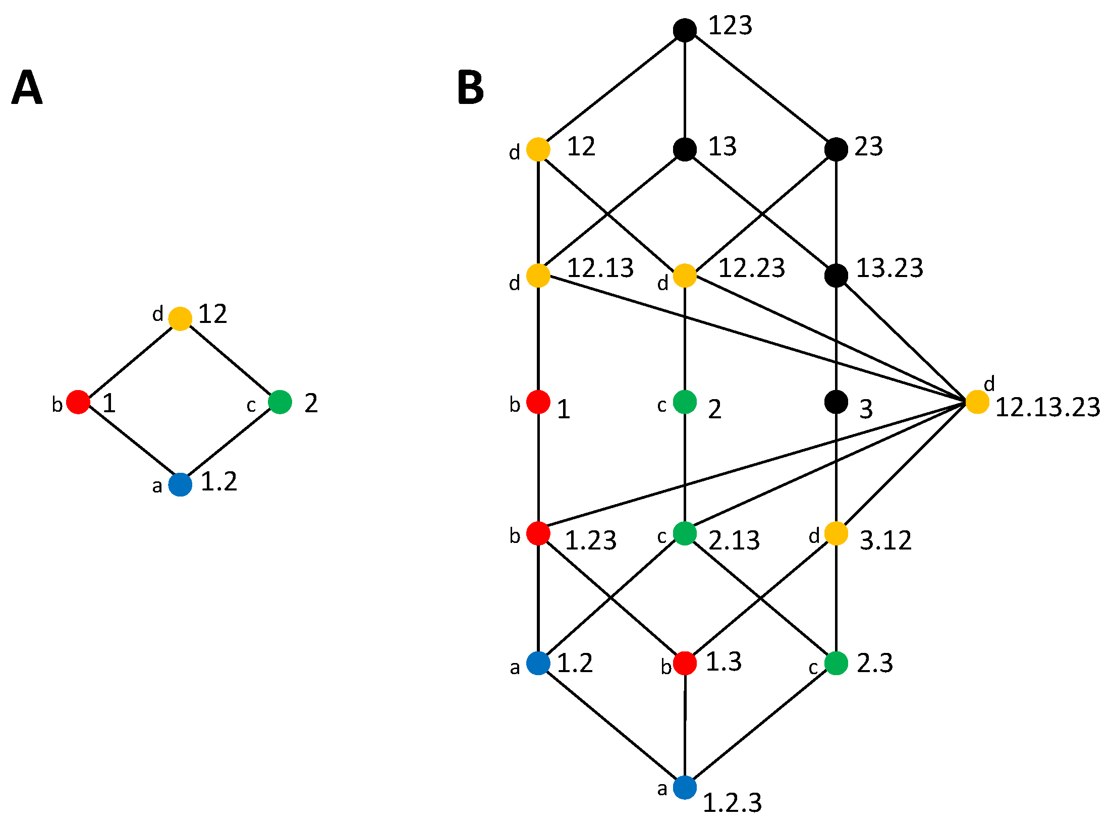
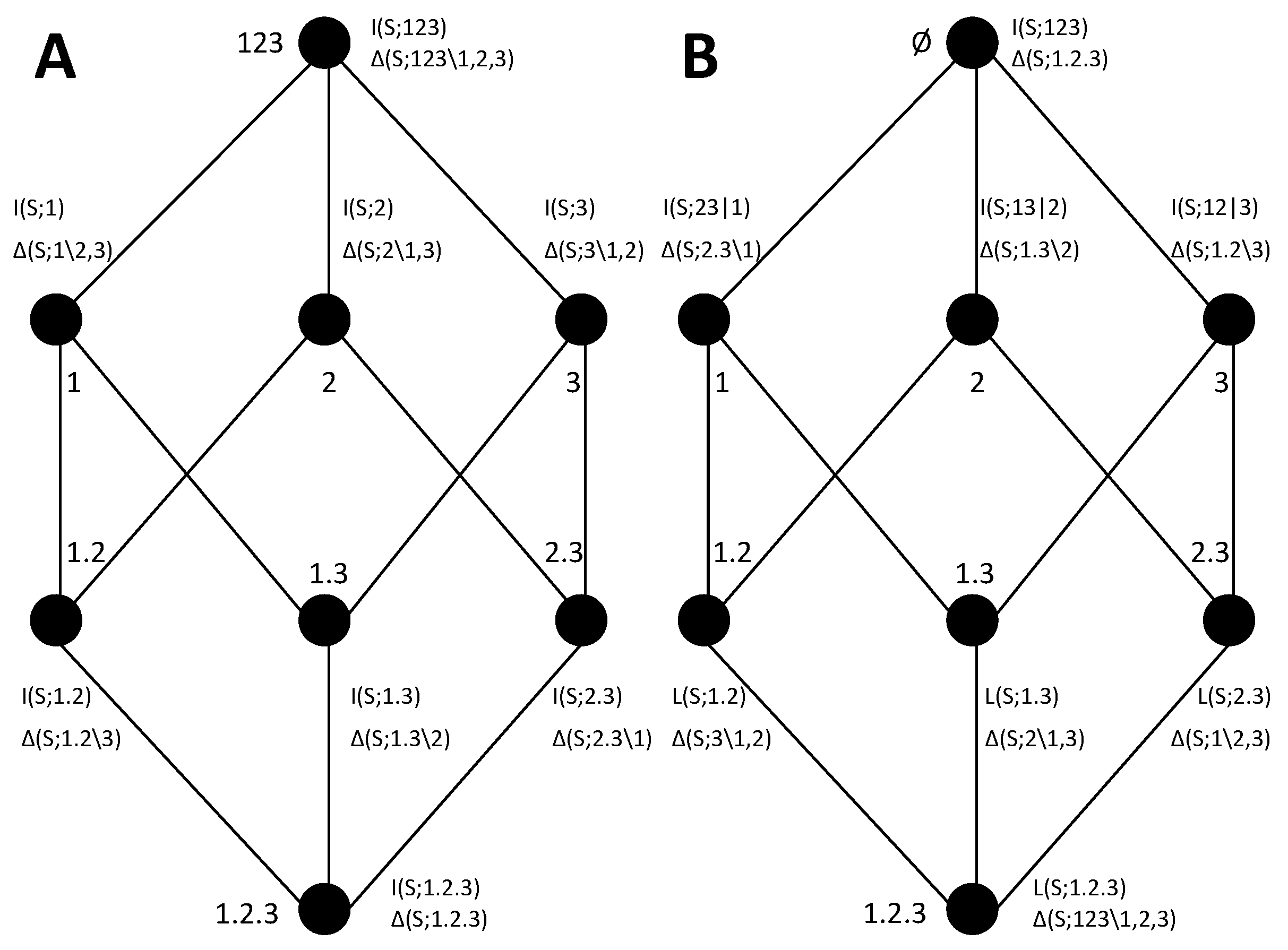
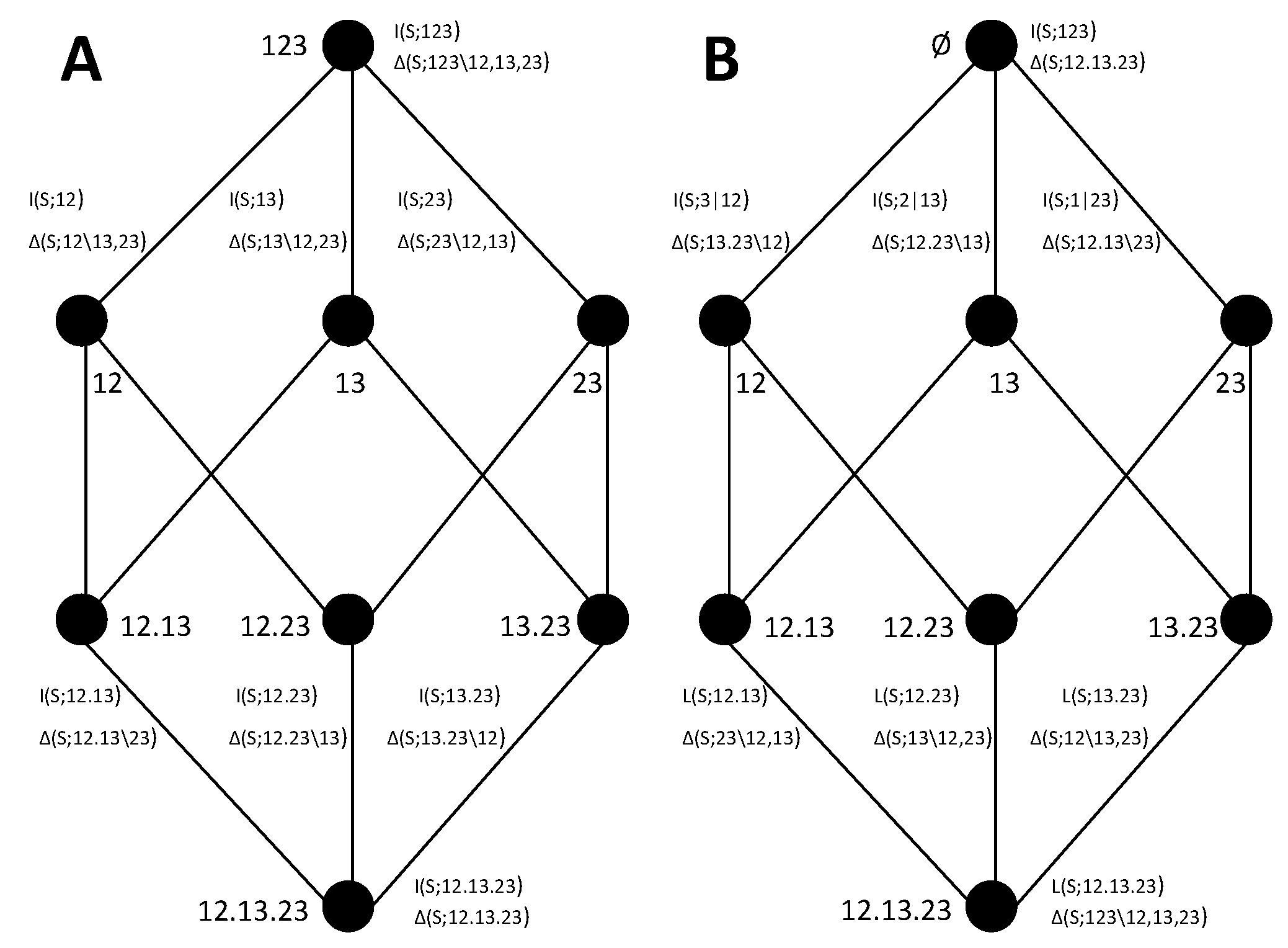
that is, for two collections α and β, $\alpha ⪯\beta$ if for each source in β there is a source in α that is a subset of that source. This ordering relation is reflexive, transitive, and antisymmetric. The lattices constructed for the case of $n=2$ and $n=3$ using this ordering relation are shown in Figure 1A,B. The order is partial because an order does not exist between all pairs of collections, for example between the collections at the same level of the lattice. In this work, we use a different notation than in [21], which allows us to shorten the expressions a bit. For example, instead of writing $\left\{1\right\}\left\{23\right\}$ for the collection composed by the source containing variable 1 and the source containing variables 2 and 3, we write $1.23$, that is, we save the curly brackets that indicate for each source the set of variables and we use instead a dot to separate the sources.

Each collection in the lattice is associated with a measure of the redundancy between the sources composing the collection. Reference [21] defined a measure of redundancy, called $I_{min}$, that is well defined for any collection. In this work, we do not need to consider the specific definition of $I_{min}$. What is relevant for us is that, when ascending the lattice, $I_{min}$ monotonically increases, being a cumulative measure of information and reaching the total amount of information at the top of the lattice. Based on this accumulation of information, we will from now on refer to the type of lattices introduced by [21] as information gain lattices. Furthermore, we will generically refer to the terms quantifying the information accumulated in each collection as cumulative terms and denote the cumulative term of a collection α by $I(S,\alpha )$. The reason for this change of terminology will become evident when we introduce the information loss lattices, since redundancy is not specific to the information gain lattices and it appears also in the loss lattices but not associated with cumulative terms, and thus we need to disentangle it nominally from the cumulative terms, even if in the formulation of [21] they are inherently associated.

Independently of which measure is used to define the cumulative terms $I(S,\alpha )$, two axioms originally required by [21] ensure that these terms and their relations are compatible with the lattice. First, the symmetry axiom requires that $I(S,\alpha )$ is invariant to the order of the sources in the collection, in the same way that the domain $\mathcal{A}\left(\mathbf{R}\right)$ of collections does not distinguish the order of the sources. Second, the monotonicity axiom requires that $I(S,\alpha )\le I(S,\beta )$ if $\alpha ⪯\beta$. Another axiom from [21] ensures that the cumulative terms are linked to the actual mutual information measures of the variables. In particular, the self-redundancy axiom requires that, when the collection is formed by a single source $\alpha =\mathbf{A}$, then $I(S;\alpha =\mathbf{A})=I(S;\mathbf{A})$, that is, the cumulative term is equal to the directly calculable mutual information of the variables in $\mathbf{A}$. The other axioms that have been proposed are not related to the construction of the information gain lattice itself. Conversely, they are motivated by desirable properties of a measure of redundancy or desirable properties of the terms in the decomposition, such as the nonnegativity axiom. The fulfillment of a proper set of additional axioms is important to endow this type of mutual information decompositions with a meaning, regarding how to interpret each component of the decomposition. However, these additional axioms do not determine, nor are they determined, by the properties of the lattice. We will not examine these other axioms in detail in this work, but we refer to Appendix C for a discussion of the requirements to obtain nonnegative terms in the decomposition.

The mutual information decomposition was constructed in [21] by implicitly defining partial information measures associated with each node, such that the cumulative terms are obtained from the sum of partial information measures:

$$I(S,\alpha )=\sum _{\beta \in \downarrow \alpha }{\Delta }_{\mathcal{C}}(S;\beta ).$$

(7)

In particular, $\downarrow \alpha$ refers to the set of collections lower than or equal to α, given the ordering relation (see Appendix A for details). Again, here we will adopt a different terminology and we will refer to ${\Delta }_{\mathcal{C}}(S;\beta )$ as the incremental term of the collection β in lattice $\mathcal{C}$, instead of as the partial information measure. This is because, as we will see, it is convenient to consider incremental terms as increments that can equally be of information gain or information loss. Given the link between the cumulative terms and the mutual information of the variables imposed by the self-redundancy axiom, the decomposition of the total mutual information results from applying Equation (7) to the collection $\alpha =\left\{\mathbf{R}\right\}$. As proved in (Theorem 3, [21]), Equation (7) can be inverted to:

$$\begin{array}{cc}\hfill {\Delta }_{\mathcal{C}}(S;\alpha )& =I(S;\alpha )-\sum _{k=1}^{|{\alpha }^{-}|}{(-1)}^{k-1}\sum _{\begin{array}{c}\mathcal{B}\subseteq {\alpha }^{-}\\ \left|\mathcal{B}\right|=k\end{array}}\sum _{\beta \in {\displaystyle \bigcap _{\gamma \in \mathcal{B}}}\downarrow \gamma }{\Delta }_{\mathcal{C}}(S;\beta )\hfill \end{array}$$

(8a)

$$\begin{array}{cc}& =I(S,\alpha )-\sum _{k=1}^{|{\alpha }^{-}|}{(-1)}^{k-1}\sum _{\begin{array}{c}\mathcal{B}\subseteq {\alpha }^{-}\\ \left|\mathcal{B}\right|=k\end{array}}I(S;\bigwedge \mathcal{B}),\hfill \end{array}$$

(8b)

where ${\alpha }^{-}$ is the cover set of α and $\bigwedge \mathcal{B}$ is the infimum of the set $\mathcal{B}$. The cover set of α is composed by the collections that are immediate descendants from α in the lattice. The infimum of a set of collections is the upper collection that can be reached descending from all collections of the set. We will also refer to the set formed by all the collections for which cumulative terms determine the incremental term ${\Delta }_{\mathcal{C}}(S;\alpha )$ as the increment sublattice $◊\alpha$. This sublattice is formed by α and by all the collections that appear as infimums in the summands of Equation (8b). See Appendix A for details on the definition of these concepts and other properties of the lattices.

3. Extended Information Gain Decompositions from Redundancy, Uniqueness or Synergy Measures

In this section, we still focus on the information gain decompositions introduced by [21]. We first extend their approach to comprise a more general set of lattices, built based on subsets of the domain of collections determined in Equation (5). We study the relation between the terms from different lattices, showing how the incremental terms of the full lattice are mapped to the incremental terms of smaller lattices. We also indicate that the existence of deterministic relations between the variables imposes constraints to the range of valid lattices. We then show that considering the connection between different lattices is not only useful to better interpret the decompositions based on a subset of collections, but also in practice provides a way to build multivariate decompositions. In particular, we introduce an iterative hierarchical procedure to build multivariate decompositions from synergy or unique information measures, something that was not possible from the full lattices alone.

3.1. Relations between Information Gain Decompositions with Different Subsets of Sources Collections

Reference [21] studied how to decompose the mutual information in decompositions composed by all the collections of sources in $\mathcal{A}\left(\mathbf{R}\right)$. Figure 1A,B show the corresponding lattices for $n=2$ and $n=3$, respectively. However, the number of collections in these decompositions rapidly increases when the number of variables increases (e.g., 7579 collections for $n=5$ [21]), which may render the decompositions difficult to handle in practice. Here, we generalize their approach in a straightforward way, considering decompositions composed by any subset $\mathcal{C}\subseteq \mathcal{A}\left(\mathbf{R}\right)$ whose elements still form a lattice (see Appendix C for a discussion of more general decompositions based on subsets that do not form a lattice). Given that the ordering relation of Equation (6) is a pairwise relation that does not depend on the set of collections considered, any lattice is built following the same rule as in the full lattice: each collection is connected by an edge to the collections in its cover set (see Appendix A), which depends on the subset of collections used to construct the lattice. For example, Figure 1C shows the decomposition formed by the collections that combine the sources 1 and 23. In Figure 1B, the red edges indicate the decomposition based on collections combining the sources 12, 13, 23, without further decomposing the contribution of single variables separately. Oppositely, Figure 1D shows the decomposition based on the sources 1, 2, and 3, which does not include bivariate sources resulting from merging these univariate sources. A certain decomposition can be embedded within a bigger one, as indicated in Figure 1B, but generally considering more collections alters the structure of the lattice, by modifying the cover relations between the nodes. For example, the decomposition of Figure 1D is not embedded in Figure 1B. Similarly, the cover relations in the bivariate decomposition of $\mathcal{A}\left(\right\{1,2\left\}\right)$ in Figure 1A change in the trivariate decomposition of $\mathcal{A}\left(\right\{1,2,3\left\}\right)$ in Figure 1B since nodes $12.13$ and $12.23$ appear between 12 and 1 and 2, respectively. The same occurs between $1.2$ and 1 and 2, with nodes $1.23$ and $2.13$, respectively. Furthermore, the down set of 12, in comparison to the bivariate lattice, comprises others nodes because of the presence of $12.13.23$.

When studying multivariate systems, the nature and relation between the variables may provide some a priori information in favor of a certain decomposition. For example, in the case of Figure 1C, variables 2 and 3 can correspond to two signals recorded from the same subsystem, while 1 is a signal from a different subsystem. This may render a bivariate decomposition more adequate, even if having three variables. For example, this is a common scenario when recording brain signals from different brain areas and the analysis of interactions can be carried out at different spatial scales [8]. Similarly, in the case of Figure 1D, one may prefer to simplify the analysis without explicitly considering all synergistic contributions of bivariate sources. Another possibility is that, even if it is known that a system is composed by a certain number of variables, only a subset is available for the analysis, and it is thus important to understand how the influence of the missing variables is reflected in each term of the decomposition. For example, if in a trivariate system only 1 and 2 are observed, we would like to understand how the terms in the full decomposition for $n=3$ are reflected in the full decomposition for $n=2$ restricted to 1 and 2. Again, this is a common scenario when studying neural population coding of sensory stimuli, since usually only simultaneous recordings from a subset of the neural population, or from one of the brain regions involved, is available. In any case, in order to better choose the most useful decomposition given a certain set of concrete variables, and to understand how the different decompositions are related, we need to consider how the terms from one decomposition are mapped to another. Furthermore, as we will see in Section 3.3, the relationship between lattices has also practical applications to build multivariate decompositions from synergy or unique information measures.

The connection between the terms in two different decompositions is qualitatively different for the cumulative terms, $I(S,\alpha )$, and the incremental terms ${\Delta }_{\mathcal{C}}(S;\alpha )$. A cumulative term $I(S,\alpha )$ quantifies the information about S that is redundant within a certain collection of sources α. This information is well defined without considering which is the set $\mathcal{C}$ of collections that has been selected, that is, it depends only on S and α. Accordingly, the cumulative terms of information gain $I(S,\alpha )$ are invariant across decompositions. Oppositely, as we here explicitly indicate in our notation, the incremental terms ${\Delta }_{\mathcal{C}}(S;\alpha )$ are, in general, decomposition-dependent. Although Equation (8) was derived in [21] only to express the incremental terms as a function of cumulative terms in the full lattices, it is straightforward to check that, by construction, the relation of Equation (7) also can be inverted to Equation (8) in lattices formed by subsets of $\mathcal{A}\left(\mathbf{R}\right)$ (See Appendix C). From Equation (8), it can be seen that the cumulative terms used to calculate ${\Delta }_{\mathcal{C}}(S;\alpha )$ depend on the specific structure of the lattice, in particular on which is the increment sublattice $◊\alpha$. This is summarized indicating that:

$$I(S;\alpha )=I_{\mathcal{C}}(S;\alpha )=I_{{\mathcal{C}}^{\prime }}(S;\alpha ),\forall \mathcal{C},{\mathcal{C}}^{\prime },$$

(9)

while for the incremental terms, only a sufficient condition for equality across decompositions can be formulated:

$${◊}_{\mathcal{C}}\alpha ={◊}_{{\mathcal{C}}^{\prime }}\alpha \Rightarrow {\Delta }_{\mathcal{C}}(S;\alpha )={\Delta }_{{\mathcal{C}}^{\prime }}(S;\alpha ),$$

(10)

which is a direct consequence of Equation (9) given the dependence of the incremental terms on the cumulative terms (Equation (8)).

The invariance of cumulative terms implies that each cumulative term that is present in two decompositions provides an equation that relates the incremental terms in those decompositions, since in each lattice cumulative terms result from the accumulation of increments according to Equation (7). In particular, for two decompositions $\mathcal{C}$ and ${\mathcal{C}}^{\prime }$ with a common collection α

$$I(S;\alpha )=\sum _{{\beta \in \downarrow }_{\mathcal{C}}\alpha }{\Delta }_{\mathcal{C}}(S;\beta )=\sum _{{\beta \in \downarrow }_{{\mathcal{C}}^{\prime }}\alpha }{\Delta }_{{\mathcal{C}}^{\prime }}(S;\beta ).$$

(13)

In general, these type of relations impose some constraints that involve several incremental terms from each decomposition. For example, when connecting the incremental terms of the decompositions of Figure 1A,C, we get only the constraint ${\Delta }_A(S;1)+{\Delta }_A(S;1.2)={\Delta }_C(S;1)+{\Delta }_C(S;1.23)$, given the only common node $I(S;1)$. An important type of comparison is between full lattices of different order. In this case, the constraints allow breaking down each of the incremental terms of the lower order lattice as a sum of incremental terms from the higher order lattice. Figure 2 shows the case for $n=2,3$ when the set $\mathcal{A}\left(\right\{1,2\left\}\right)$ of the full decomposition for $n=2$ is a subset of $\mathcal{A}\left(\right\{1,2,3\left\}\right)$, corresponding to the full decomposition for $n=3$. This determination of each incremental term of one lattice as a function of the incremental terms of another lattice holds, in general, when the set of collections of the smaller lattice is a subset of the collections used in the bigger lattice. This happens not only when comparing a full lattice with a full lattice of lower order (Figure 2), but also for $n=3$ in Figure 1B, when comparing a full lattice with any lattice composed by a subset of the collections (Figure 1A,C,D).

Figure 3A,B further shows how the incremental terms of the sublattice of Figure 1D can be broken down as a sum of the incremental terms of the full lattice. However, in general, the fact that each incremental term of the smaller lattice can be expressed as a combination of the incremental terms of the bigger lattice, does not mean that each incremental term of the latter is related to a single incremental term of the former. This is illustrated in Figure 3C,D. The set of collections of the lattice in Figure 3C is a subset of the set of the lattice in Figure 3D. However, now each incremental term of Figure 3D contributes to more than one incremental term of Figure 3C. For example, ${\Delta }_C(S;1)={\Delta }_D(S;2)+{\Delta }_D(S;1.2)+{\Delta }_D(S;2.3)$, but also ${\Delta }_C(S;1)={\Delta }_D(S;1)+{\Delta }_D(S;1.2)+{\Delta }_D(S;1.3)$, with ${\Delta }_D(S;1.2)$ contributing to both. Furthermore, since the incremental terms of the full lattice can only contribute once to the decomposition of $I(S;123)$, the fact that an incremental term of Figure 3D contributes twice positively, is balanced by a negative contribution to another incremental term of Figure 3C. Combining the correspondences of Figure 3C,D and Figure 3A,B, we can see that the incremental terms of the full lattice of Figure 3B contribute in an overlapping way to the incremental terms of Figure 3C, that is, there is no function assigning a single term in Figure 3C to the terms of the full lattice. To understand which lattices produce overlapping projections, let us examine in more detail the constraint of Equation (11) for $I(S;1)$ and $I(S;2)$ in the lattices of Figure 3C,D. Each cumulative term is obtained as the sum of all incremental terms from nodes reached descending from the node of the cumulative term (Equation (7)). In Figure 3D, $1.2$ is the infimum of 1 and 2, that is, the first node common to the descending paths from 1 and 2. This means that the incremental terms from this infimum and nodes reached descending from it contribute to both $I(S;1)$ and $I(S;2)$. If these nodes are not present in Figure 3C, then some upper incremental term will have to account for them. In this case, the node $1.2.3$ is present in Figure 3C, but $1.2$ is not and thus has to be accounted for both in the incremental terms of 1 and 2. This type of loss of the infimum node does not occur when the full lattice is reduced to the one of Figure 3A. For example, the infimum of 1 and 2 is $1.2$ and this node is preserved, even if the intermediate nodes $1.23$ and $2.13$ are not. Therefore, in general, preserving the structure of the infimums when taking a subset of $\mathcal{A}\left(\mathbf{R}\right)$ to construct a lattice is what determines if a non-overlapping projection exists or not. If for two collections in the subset their infimum collection is not included, then Equation (7) can only be fulfilled for both cumulative terms by a multiple contribution of the incremental term of the infimum in the full lattice to the incremental terms of the smaller lattice.

3.2. Checking the Validity of Lattices in the Presence of Deterministic Relations between the Variables

As a last remark regarding the selection of different lattices we indicate that, when deterministic relationships exist between the variables, the definition of the domain of collections (Equation (5)) and the ordering relation (Equation 6) can impose some limitations on the decompositions that are possible. In particular, Equation (5) excludes any collection in which a source is a superset of any other. Consider, for example, the case of three variables $1,2,3$ such that 12 completely determine 3. Accordingly, in the decomposition of Figure 1B, several collections are altered, since the source 12 could be replaced by 123. This leads to the presence of invalid collections in the set, such as $123.13$ instead of $12.13$, since 13 is a subset of 123. Similarly, given the deterministic relation, one could reduce 123 to 12, duplicating this last collection and affecting the ordering relation of the top element with 13 and 23. In general, this means that a certain lattice cannot be taken as valid a priori. Conversely, it should be verified, for each specific set of variables, if the collections that compose it are valid once the properties of the variables are taken into account.

The exclusion of certain lattices in the presence of deterministic relations can be seen as a limitation of the decomposition framework, but on the other hand this verification turns out to be important to avoid problematic cases. In particular, it allows avoiding the counterexample provided in [26] to show that it is not always possible when $n>2$, independently of how the terms of the decomposition are defined, to obtain a nonnegative decomposition. This counterexample is based on three variables such that any pair deterministically determines the third. Without using any specific definition of the measures associated with the nodes, the authors proved that at least a certain incremental term of the lattice of Figure 1B is negative in this case. However, given the deterministic relations between the variables, all the collections comprising a bivariate source need to be excluded from the set, since these bivariate sources are equivalent to the source 123 and thus any other source in the collection is a subset of this one. Similarly, 123 can be reduced to any collection containing a single source composed by a pair of the variables, which duplicates these collections and affects the ordering relations. In Appendix B, we reconsider in more detail the counterexample of [26]. We show that taking into account the deterministic relations leads to the construction of a smaller lattice that complies the constraints of Equations (5) and (6) and for which nonnegativity is preserved. Therefore, we can reinterpret the violation of the nonnegativity axiom as a more specific non-compliance of the constraints for a certain set of variables. However, note that the possibility to deal with cases such as the one raised in [26] by adapting the lattice does not preclude from the potential existence of negative incremental terms. As we reviewed above, the definition of the proper measure for the decompositions is an open question, and finding a measure that ensures generally the nonnegativity of the incremental terms, or identifying the properties of the variables or the decompositions that ensures this nonnegativity, is out of the scope of this work. Only in Appendix C we review the requirements to obtain nonnegative incremental terms. For this purpose, we reexamine from a more general perspective several of the Theorems of [21], identifying the key ingredients of the proofs that are sustained by lattice properties, by general properties captured in the axioms that have been proposed [22], or by properties specific of their measure $I_{min}$.

3.3. An Iterative Hierarchical Procedure to Determine Information Gain Cumulative Terms from Synergy or Unique Information Measures by Combining Information Gain Decompositions of Different Orders

Above, we have examined possible alternative decompositions of the mutual information and the relations among them from a generic perspective, based only on the structure of the decompositions and the general properties of the cumulative and incremental terms. Apart from the general advantage of understanding these relations in order to select and interpret the decompositions, we now show that these relations also have a more immediate practical implication and provide a way to determine the components of multivariate decompositions when the cumulative terms are not predefined but only a measure that can be associated with certain incremental terms is used as the basis to construct the decomposition. If a measure of accumulated mutual information gain $I(S,\alpha )$ is defined, it is straightforward to calculate all the terms in the decomposition. The cumulative terms are already defined based on this measure and the incremental terms can be calculated using Equation (8). This was the case in the seminal work of [21], where the cumulative terms were defined as the redundancy measures $I_{min}$. However, the calculation of all terms is not straightforward if the measure defined as the basis to construct the decomposition does not define the cumulative terms. In fact, in the different proposals that exist so far, the basic component chosen to calculate the other terms has alternatively been a redundancy measure [21,22,25,32], a synergy measure [23], or a unique information measure [24]. When the measure of redundancy is sufficiently general to be taken as a general definition of all cumulative terms, the multivariate decompositions can be built in a direct way. Conversely, when a measure of synergy or unique information is taken as the basis, only bivariate decompositions can be directly built and only bivariate decompositions have been studied [23,24]. To our knowledge, there is currently no general procedure to construct the decomposition associated with an information gain lattice in the multivariate case from the definition of a measure of synergy or unique information. We here describe an iterative hierarchical procedure to do so, which relies on the relations between lattices of different order.

We start by considering first the bivariate case, to understand why, in this case, the lattice can be constructed from synergy or unique information measures in a simple way and why this procedure does not apply directly for the multivariate case. In the bivariate case, Equations (1) and (2) provide $m=3$ equations to relate the $K=4$ terms of the bivariate decomposition with $I(S;1)$, $I(S;2)$, and $I(S;12)$, so that defining one of the four terms is enough to identify the other three. However, this direct procedure cannot similarly be applied for $n>2$. This can be understood, already for $n=3$, considering the number of cumulative terms which are directly calculable as a mutual information thanks to the self-redundancy axiom. These terms are the ones related to the collections formed by a single source, 1, 2, 3, 12, 13, 23, and 123. This means that only $m=7$ equations analogous to Equations (1) and (2) are available to calculate the $K=18$ cumulative terms. If the measure taken as basis of the decomposition is defined generally for each node (as $I_{min}$ in [21]) this is not a problem, and these seven equations are directly fulfilled as special cases of Equation (7). However, if the measure taken as the basis is a measure of synergy or uniqueness, then it does not define directly the cumulative terms, but only certain incremental terms. This difference is clear already for $n=2$. The redundancy $I(S;1.2)$ is a cumulative term in the decomposition, in particular it corresponds to the bottom element of the lattice. Conversely, the unique information terms $I(S;1\backslash 2)$ and $I(S;2\backslash 1)$, as well as the synergy $I(S;12\backslash 1,2)$ correspond to incremental terms. That is, the particularity of redundancy measures such as $I_{min}$ is that they provide a definition for all the cumulative terms of the mutual information gain decomposition, while the measures of unique information or synergy, for $n>2$, do not provide a definition applicable to all the incremental terms of the lattice.

We will now describe a new iterative hierarchical procedure to build information gain multivariate decompositions from measures of synergy or unique information. For simplicity, we will focus on the case of $n=3$, but the logic of the procedure can be extrapolated to the general multivariate case. As we will show in Section 4 by introducing the alternative information loss lattices, this is not the only way to build these multivariate decompositions. In fact, this procedure can lead to some inconsistencies if it is applied to any lattice without a careful examination of the correspondence between incremental terms and synergy or unique information measures. However, if the lattices and measures are properly chosen, as we will discuss after introducing the dual decompositions of information gain and information loss in Section 5, the different procedures to build multivariate decompositions are consistent and the same cumulative terms and incremental terms are obtained independently of how they are calculated.

The key ingredient for this procedure is the invariance of the cumulative terms across decompositions, as indicated in Equation (9). Based on this invariance, we can resort to the bivariate decompositions in order to calculate many of the cumulative terms of the trivariate decomposition of Figure 1B. Indeed, from the 18 minus 7 terms that do not correspond directly to the mutual information of a single source, all except the ones of the collections $12.13.23$ and $1.2.3$ appear also in a bivariate decomposition. For example, $1.2$ is part of the decomposition in Figure 1A, and $1.23$ is part of the one in Figure 1C. Analogous bivariate decompositions exist for $1.3$, $2.3$, $2.13$, $3.12$, $12.13$, $12.23$, and $13.23$. For each of these bivariate decompositions, if a definition of bivariate synergy is defined, it can be used to determine the corresponding bivariate redundancy, which, being a cumulative term, is invariant and can be used equally in the trivariate decomposition. Accordingly, it is the connection between different decompositions what allows us to calculate most of the terms. This same procedure of using the bivariate decompositions could be used if instead of a definition of synergy, we used a definition of unique information. Finally, to calculate $1.2.3$ and $12.13.23$, we can use the smaller trivariate decompositions of Figure 1D and the one composed by the red edges of Figure 1B, respectively. In these two smaller trivariate decompositions, after using the bivariate ones to calculate the corresponding cumulative terms, the situation becomes the same as for the bivariate case: all cumulative terms are already calculated except one, which means that it suffices to define a single measure, either a synergy or unique information, in order to be able to retrieve the complete set of cumulative and incremental terms.

This procedure provides a way to construct multivariate decompositions, simply by recurrently using decompositions of a lower order to calculate the cumulative terms. Since the cumulative terms are invariant, at each order, most of them are not specific of that order and appear also in lattices of lower orders. However, this approach leads to some inconsistencies if it is applied to any lattice without carefully considering how a synergy or unique information measure can be associated with an incremental term. In particular, consider that a measure of synergy is provided, which should allow identifying the top incremental term of any of the decompositions used in the iterative procedure. For example, a measure of synergy should determine the incremental term $\Delta (S;123\backslash 12.13.23)$ of Figure 1B and $\Delta (S;123\backslash 1.2.3)$ of Figure 1D. However, the same measure of synergy cannot be taken to determine the same top incremental term $\Delta (S;123\backslash 1.2.3)$ of Figure 1D for other lattices, since the incremental terms are decomposition-specific. For example, consider the alternative decompositions presented in Figure 4A,B, and Figure 4C,D, respectively. In Figure 4A,B, if the same definition of $\Delta (S;123\backslash 1.2.3)$ is used based on the synergy measure, this results in a different form for $I(S;1.2.3)$ in the two lattices, because the increment sublattices ${◊}_{A}123\ne {◊}_{B}123$. This contradicts the invariance of the cumulative terms across lattices. Figure 4C,D presents another contradiction resulting from directly using the same synergy definition: since collections 123, 1, and 23 are common to both decompositions, the same expression would be obtained for the redundancy $I(S;1.23)$ and $I(S;1.2.3)$ depending on the lattice used. For both examples, the problem is that a definition of synergy is expected to depend only on S and on the sources among which synergy is quantified, but cannot be context-dependent, in opposition to the incremental terms, which are always context-dependent in the sense that they are decomposition-specific.

In more detail, given the conceptual meaning of synergy, when a synergy measure is to be associated with an incremental term, the precise synergy contribution to be quantified is only determined by the collection α and the collections on its cover ${\alpha }^{-}$. For example, in Figure 4A, $\Delta (S;123\backslash 1.2.3)$ quantifies the overall synergistic increase in information that can arise from combining any of the single variables. However, the incremental term is not only determined by α and ${\alpha }^{-}$, conversely, it depends on the whole increment sublattice $◊\alpha$. We have seen in Figure 3C,D that $\Delta (S;123\backslash 1.2.3)$ is a different incremental term for these lattices, with a different expression as a function of the incremental terms of the full lattice. Accordingly, it is not straightforward to interpret the top incremental term as the one quantifying the synergistic component of the mutual information, since different possible decompositions result in different terms. This issue does not arise for the bivariate decomposition because a single decomposition involving a synergistic component is possible. In general, for a given definition of synergy or unique information, or more generally for any measure which is conceptually defined in order to capture a certain portion of the total mutual information (e.g., the union-information in [23]), the incremental terms to which the measure can be associated is not directly determined by the local structure of the lattice related to the variables involved in the definition of the measure, but by the whole incremental sublattice. The meaning of the measure assigned to an incremental term has to be consistent with its expression as a function of the incremental terms of the full lattice. Only with this careful examination of the correspondence between measures and incremental terms, the iterative procedure can be used to build multivariate decompositions.

4. Decompositions of Mutual Information Loss

Although the iterative hierarchical procedure allows determining the information gain decompositions from a synergy measure, the construction has to proceed in a reversed way, determining the cumulative terms from the incremental terms using lower order lattices. This means that the full lattice at a given order cannot be determined separately, but always by jointly constructing a range of lower order lattices. We now examine if this asymmetry between redundancy measures, corresponding to cumulative terms, and synergy measures, corresponding to incremental terms, is intrinsic to the notions of redundancy and synergy, or if conversely this correspondence can be inverted. Indeed, we introduce the type of information loss lattices in which synergy is associated with cumulative terms and redundancy with incremental terms. Apart from the implications of the possibility of this inversion in the understanding of the nature synergy and redundant contributions, a practical application of information loss lattices is that, using them as the basis of the mutual information decomposition, the decomposition can be directly determined from a synergy measure in the same way that it can be directly determined from a redundancy measure when using gain lattices. In Section 5, we will study in which cases information gain and loss lattices are dual, providing the same decomposition of the mutual information.

As a first step to obtain a mutual information decomposition associated with an information loss lattice, we define a new ordering relation between the collections. In the lattices associated with the decompositions of mutual information gain, the ordering relation is defined such that upper nodes correspond to collections which cumulative terms have more information about S than each of the cumulative terms in their down set. Oppositely, in the lattice associated with a decomposition of mutual information loss, an upper node corresponds to a higher loss of the total information contained in the whole set of variables about S. The domain of the collections valid for the information loss decomposition can be defined analogously to the case of information gain:

$${\mathcal{A}}^{*}\left(\mathbf{R}\right)=\{\alpha \in \mathcal{P}\left(\mathbf{R}\right)\backslash \left\{\mathbf{R}\right\}:\forall {\mathbf{A}}_i,{\mathbf{A}}_j\in \alpha ,{\mathbf{A}}_i⊈{\mathbf{A}}_j\}.$$

(12)

Note that this domain is equivalent to the one of the information gain decompositions (Equation (5)), except that the collection corresponding to the source containing all variables $\left\{\mathbf{R}\right\}$ is excluded instead of the empty collection. This is because, in the same way that no information gain can be accumulated with no variables, no loss can be accumulated with all variables. Furthermore, ${\mathcal{A}}^{*}\left(\mathbf{R}\right)$ excludes collections that contain sources that are supersets of other sources of the same collection, equally to $\mathcal{A}\left(\mathbf{R}\right)$. An ordering relation is introduced analogously to Equation (6):

$$\forall \alpha ,\beta \in {\mathcal{A}}^{*}\left(\mathbf{R}\right),(\alpha ⪯\beta \iff \forall \mathbf{B}\in \beta ,\exists \mathbf{A}\in \alpha ,\mathbf{B}\subseteq \mathbf{A}).$$

(13)

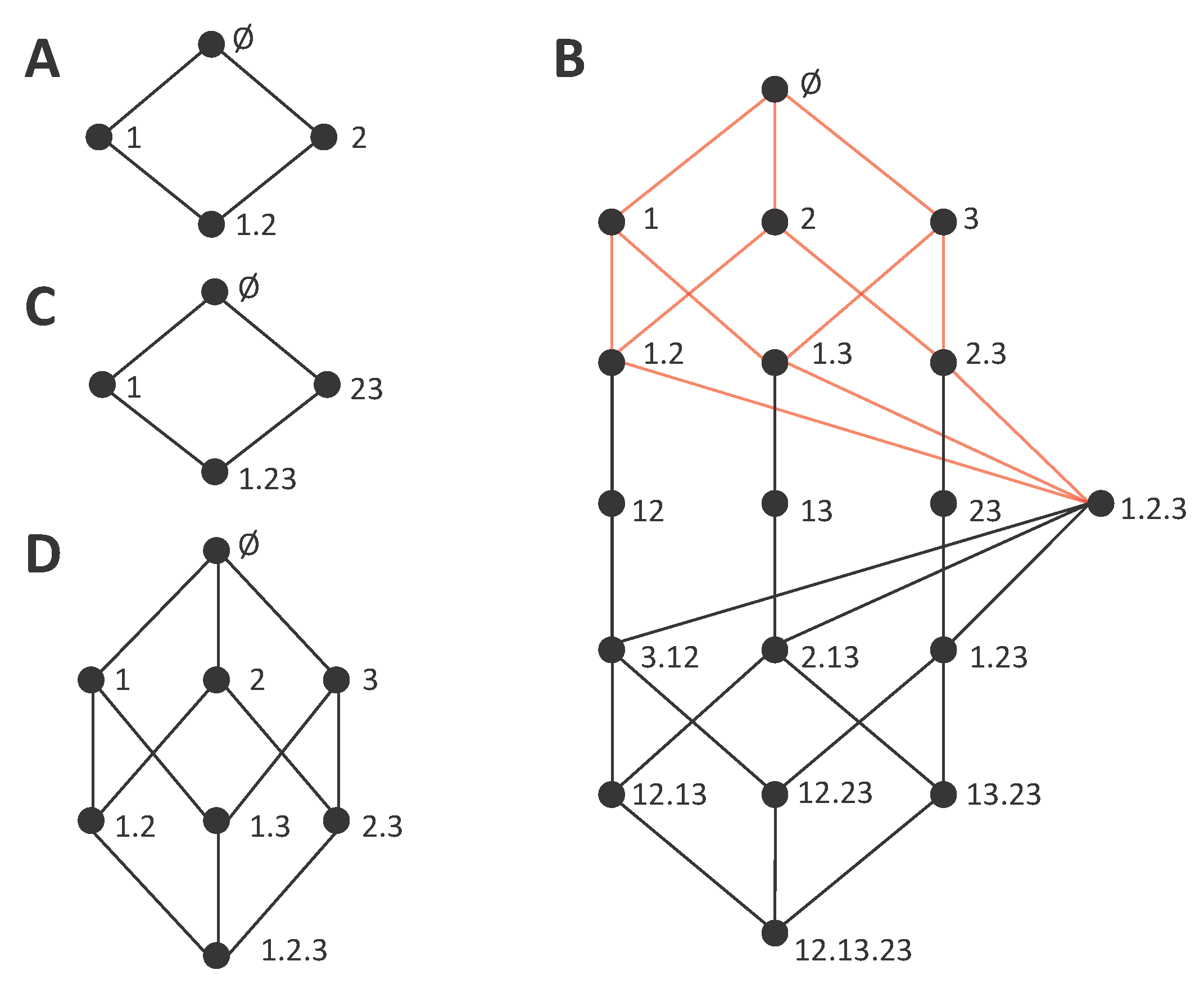
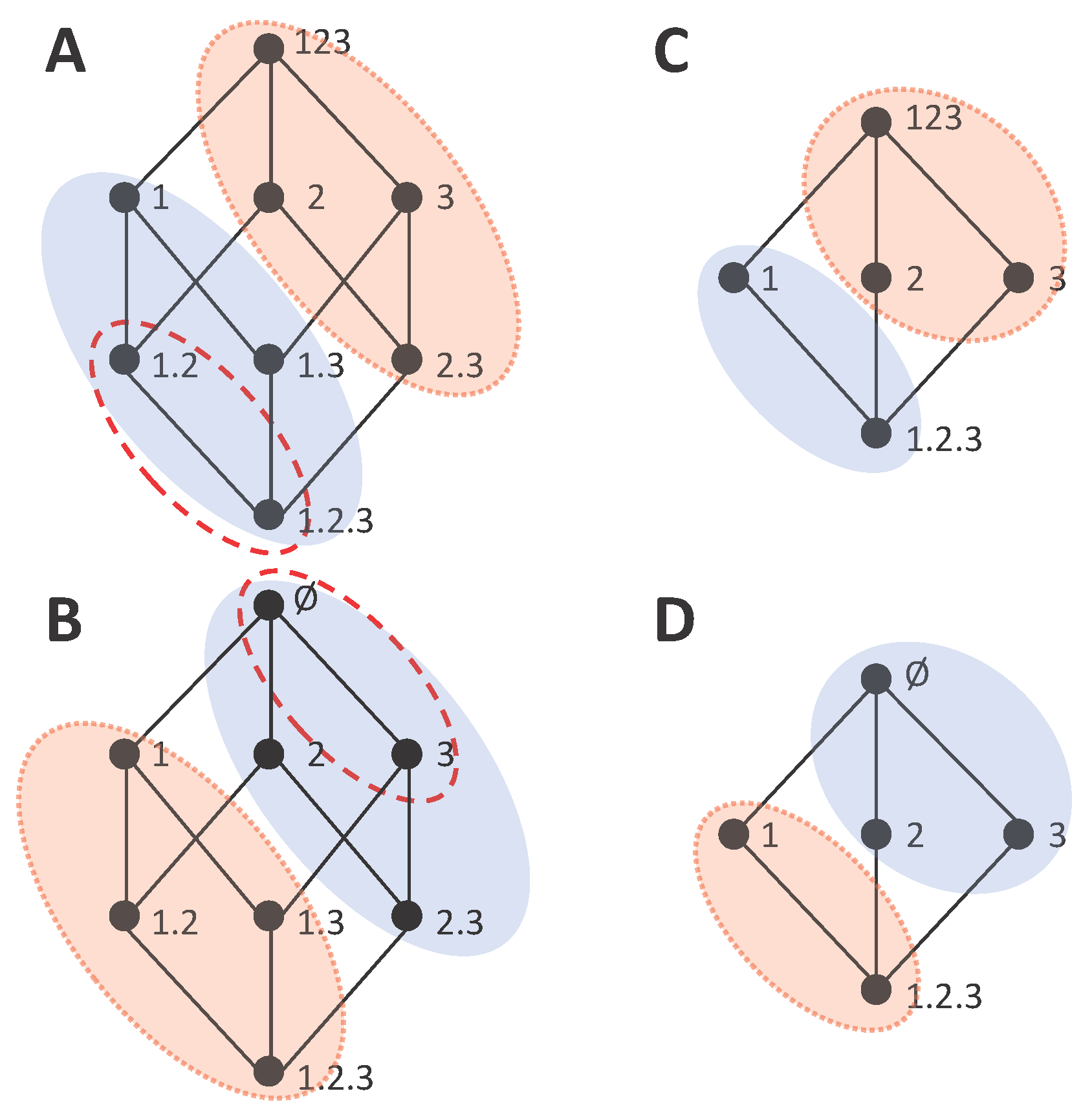
This ordering relation differs from the one of lattices associated with information gain decompositions in that now upper collections should contain subset sources and not the opposite. Figure 5 shows several information loss decompositions analogous to the gain decompositions of Figure 1. For the lattices of Figure 5A,C,D, the only difference with respect to Figure 1 is the top node, where the collection containing all variables is replaced by the empty set. Indeed, the empty set results in the highest information loss. For the full trivariate decomposition of Figure 5B, there are many more changes in the structure of the lattice with respect to Figure 1B. In particular, now the smaller embedded lattice indicated with the red edges corresponds to the one of Figure 5D, while the lattice of Figure 1D is not embedded in Figure 1B. An intuitive way to interpret the mutual information loss decomposition is in terms of the marginal probability distributions from which information can be obtained for each collection of sources. Each source in a collection indicates a certain probability distribution that is available. For example, the collection $12.13$, composed by the sources 12 and 13, is associated with the preservation of the information contained in the marginal distributions $p(S,1,2)$ and $p(S,1,3)$. Note that all distributions are joint distributions of the sources and S. In this view, the extra information contained in $p(S;\mathbf{R})$ that cannot be obtained from the marginals preserved, corresponds to the accumulated information loss. Accordingly, the information loss decompositions can be connected to hierarchical decompositions of the mutual information [33,34]. Furthermore, information loss associated with the preservation of only certain marginal distributions can be formulated in terms of maximum entropy [24], which renders loss lattices suitable to extend previous work studying neural population coding with the maximum entropy framework [15].

We will use the notation $L(S;\alpha )$ to refer to the cumulative terms of the information loss decomposition, in comparison to the cumulative terms of information gain $I(S;\alpha )$. For the incremental terms, since they also correspond to a difference of information (in this case lost information) we will use the same notation. This will be further justified below when examining the dual relationship between certain information gain and loss lattices. However, when we want to explicitly indicate the type of lattice to which an incremental term belongs, we will explicitly distinguish $\Delta I$ and $\Delta L$. Importantly, the role of synergy measures and redundancy measures is exchanged in the information loss lattice with respect to the information gain lattice. In particular, in the information loss lattices, the bottom element of the lattice corresponds to the synergistic term that in the information gain lattices is located at the top element. This represents a qualitative difference because now it is the synergy measure which is associated with cumulative terms, and redundancy is quantified by an incremental term. For example, in Figure 5B, $L(S;12.13.23)$ quantifies the information loss of considering only the sources $12.13.23$ instead of the joint source 123, which is a synergistic component. On the other hand, the incremental term $\Delta (S;\mathsf{\varnothing }\backslash 1,2,3)$ quantifies the information loss of either removing the source 1, or removing 2, or removing 3. Since the information loss quantified is associated with removing any of these sources, it means that the loss corresponds to information which was redundant to these three sources. This reasoning applies also to identify the unique nature of other incremental terms of the information loss lattice. For example, $\Delta (S;12.13\backslash 23)$ can readily be interpreted as the unique information contained in 23 that is lost when having only sources $12.13$.

Analogously to the information gain lattices, we require that the measures used for the cumulative terms fulfill the symmetry and monotonicity axioms, so that the cumulative terms inherit the structure of the lattice. We also require the fulfilment of the self-redundancy axiom, so that the cumulative terms are linked to mutual information measures of the variables when the collections have a single source. In particular, for $\alpha =\mathbf{A}$, the loss due to only using $\mathbf{A}$ corresponds to $I(S;\{\mathbf{R}\left\}\right)-I(S;\mathbf{A})$, which is the conditional mutual information $I(S;\{\mathbf{R}\left\}\right|\mathbf{A})$. That is, in the same way that the cumulative terms $I(S;\alpha =\mathbf{A})$ should be directly calculable as the mutual information of the variables, the cumulative terms $L(S;\alpha =\mathbf{A})$ should be directly calculable as conditional mutual information. Apart from these axioms directly related to the construction of the information loss lattice, we do not assume any further constraint to the measures used as cumulative terms $L(S;\alpha )$, and the selection of the concrete measures will determine the interpretability of the decomposition. Since, like in the information gain lattice, the top cumulative term is equal to the total information ($L(S;\mathsf{\varnothing })=I(S;\{\mathbf{R}\left\}\right)$), the lattice is a decomposition of the mutual information for a certain set of variables $\left\{\mathbf{R}\right\}$. In more detail, the relations between cumulative and incremental terms are defined totally equivalent to the ones of the information gain lattices

$$L(S,\alpha )=\sum _{\beta \in \downarrow \alpha }{\Delta }_{\mathcal{C}}L(S;\beta ),$$

(14)

and

$$\begin{array}{cc}\hfill {\Delta }_{\mathcal{C}}L(S;\alpha )& =L(S;\alpha )-\sum _{k=1}^{|{\alpha }^{-}|}{(-1)}^{k-1}\sum _{\begin{array}{c}\mathcal{B}\subseteq {\alpha }^{-}\\ \left|\mathcal{B}\right|=k\end{array}}\sum _{\beta \in {\displaystyle \bigcap _{\gamma \in \mathcal{B}}}\downarrow \gamma }{\Delta }_{\mathcal{C}}L(S;\beta )\hfill \end{array}$$

(15a)

$$\begin{array}{cc}& =L(S,\alpha )-\sum _{k=1}^{|{\alpha }^{-}|}{(-1)}^{k-1}\sum _{\begin{array}{c}\mathcal{B}\subseteq {\alpha }^{-}\\ \left|\mathcal{B}\right|=k\end{array}}L(S;\bigwedge \mathcal{B}).\hfill \end{array}$$

(15b)

The definition of information loss lattices simplifies the construction of mutual information decompositions from a synergy measure. If a synergy measure can generically be used to define the cumulative terms of the loss lattice analogously to how a redundancy measure, for example, $I_{min}$ defines the cumulative terms of the gain lattice, then these equations relating cumulative and incremental terms can be applied to identify all the remaining terms. Accordingly, the introduction of information loss lattices solves the problem of the ambiguity of the synergy terms derived from information gain lattices, which was caused by the identification of synergistic contributions with incremental terms, which are decomposition-specific by construction. In the information loss decomposition, the synergy contributions are identified with cumulative terms, and thus are not decomposition-specific. That is, if a conceptually proper measure of synergy is proposed, it can be used to construct the decomposition straightforwardly, without the need to examine to which terms the measure can be assigned, as it happens with the correspondence with incremental terms in the gain lattices. Note however, that there is still a difference between the degree of invariance of the cumulative terms in the information gain decompositions and in the information loss decompositions. The loss is per se relative to a maximum amount of information that can be achieved. This means that the cumulative terms of the information loss decomposition are only invariant across decompositions that have in common the set of variables from which the collections are constructed. Taking this into account, the relations between different lattices with different subsets of collections are analogous to the ones examined in Section 3.1 for the gain lattices. Similarly, an analogous iterative hierarchical procedure can be used with the loss lattices to build multivariate decompositions by associating redundancy or unique information measures to the incremental terms of the loss lattice.

5. Dual Decompositions of Information Gain and Information Loss

The existence of alternative decompositions, associated with information gain and information loss lattices, respectively, raises the question of to which degree these decompositions are consistent. A different quantification of synergy and redundancy for each lattice type would not be compatible with the decomposition being meaningful with regards to unique notions of synergy and redundancy. Comparing the information gain lattices and the information loss lattices, we see that the former seem adequate to quantify unambiguously redundancy and the latter to quantify unambiguously synergy, in the sense that there is a reverse in which measures correspond to the decomposition-invariant cumulative terms. However, we would like to understand in more detail, how the two types of lattices are connected, i.e., which relations exist between the cumulative or incremental terms of each other, and how to quantify synergy and redundancy together. We now study how information gain and information loss components can be mapped between the information gain and information loss lattices, and we define lattice duality as a set of conditions that impose a symmetry in the structure of the lattices such that for dual lattices the set of incremental terms is the same, leading to a unique total mutual information decomposition.

Considering how the total mutual information decomposition is obtained by applying Equations (7) and (14) to $I(S;\{\mathbf{R}\left\}\right)$ and to $L(S;\mathsf{\varnothing })$, respectively in the gain and loss lattices, it is clear that both types of lattices can be used to track the accumulation of information gain or the accumulation of information loss. Each node α partitions the total information in two parts: the accumulated gain (loss) and the rest of the information, which is hence a loss (gain), respectively, for each type of lattice. In particular:

$$\begin{array}{cc}\hfill I(S;\alpha )& =\sum _{\beta \in \downarrow \alpha }\Delta I(S;\beta )\hfill \end{array}$$

(16a)

$$\begin{array}{cc}\hfill I(S;\{\mathbf{R}\left\}\right)-I(S;\alpha )& =\sum _{\beta \in {(\downarrow \alpha )}^C}\Delta I(S;\beta )\hfill \end{array}$$

(16b)

$$\begin{array}{cc}\hfill L(S;{\alpha }^{\prime })& =\sum _{\beta \in \downarrow {\alpha }^{\prime }}\Delta L(S;\beta )\hfill \end{array}$$

(16c)

$$\begin{array}{cc}\hfill I(S;\left\{\mathbf{R}\right\})-L(S;{\alpha }^{\prime })& =\sum _{\beta \in {(\downarrow {\alpha }^{\prime })}^C}\Delta L(S;\beta ),\hfill \end{array}$$

(16d)

where ${(\downarrow \alpha )}^C=\mathcal{C}\backslash \downarrow \alpha$ is the complementary set to the down set of α given the particular set of collections $\mathcal{C}$ used to build a lattice. These equations indicate that in the information gain lattice all nodes (collections) out of the down set of α correspond to the information not gained by α, or equivalently, to the information loss by using α instead of the whole set of variables. Analogously, in the information loss lattice, all nodes out of the down set of ${\alpha }^{\prime }$ contain the information not lost by ${\alpha }^{\prime }$, i.e., the information gained by using ${\alpha }^{\prime }$. Accordingly, in both types of lattices, we can say that each collection α partitions the lattice into an accumulation of gained and lost information. This means that the terms $I(S;\{\mathbf{R}\left\}\right)-I(S;\alpha )$, when descending the gain lattice instead of ascending it, follow a monotonic accumulation of loss, in the same way that the terms $L(S;{\alpha }^{\prime })$ follow a monotonic accumulation of loss when ascending the loss lattice. Vice-versa, the terms $I(S;\left\{\mathbf{R}\right\})-L(S;{\alpha }^{\prime })$, when descending the loss lattice instead of ascending it, follow a monotonic accumulation of gain, in the same way that the terms $I(S;\alpha )$ follow a monotonic accumulation of gain when ascending the gain lattice. However, these equations do not establish any mapping between the gain and loss lattices. In particular, they do not determine any correspondence between $I(S;\{\mathbf{R}\left\}\right)-I(S;\alpha )$ and any cumulative term of the loss lattice and $I(S;\left\{\mathbf{R}\right\})-L(S;{\alpha }^{\prime })$ and any term of the gain lattice. They only describe how information gain and loss are accumulated within each type of lattice separately. For the mutual information decomposition to be unique, any accumulation of information loss or gain, ascending or descending a lattice, has to rely on the same incremental terms.

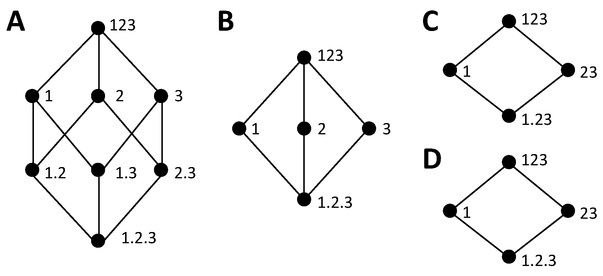
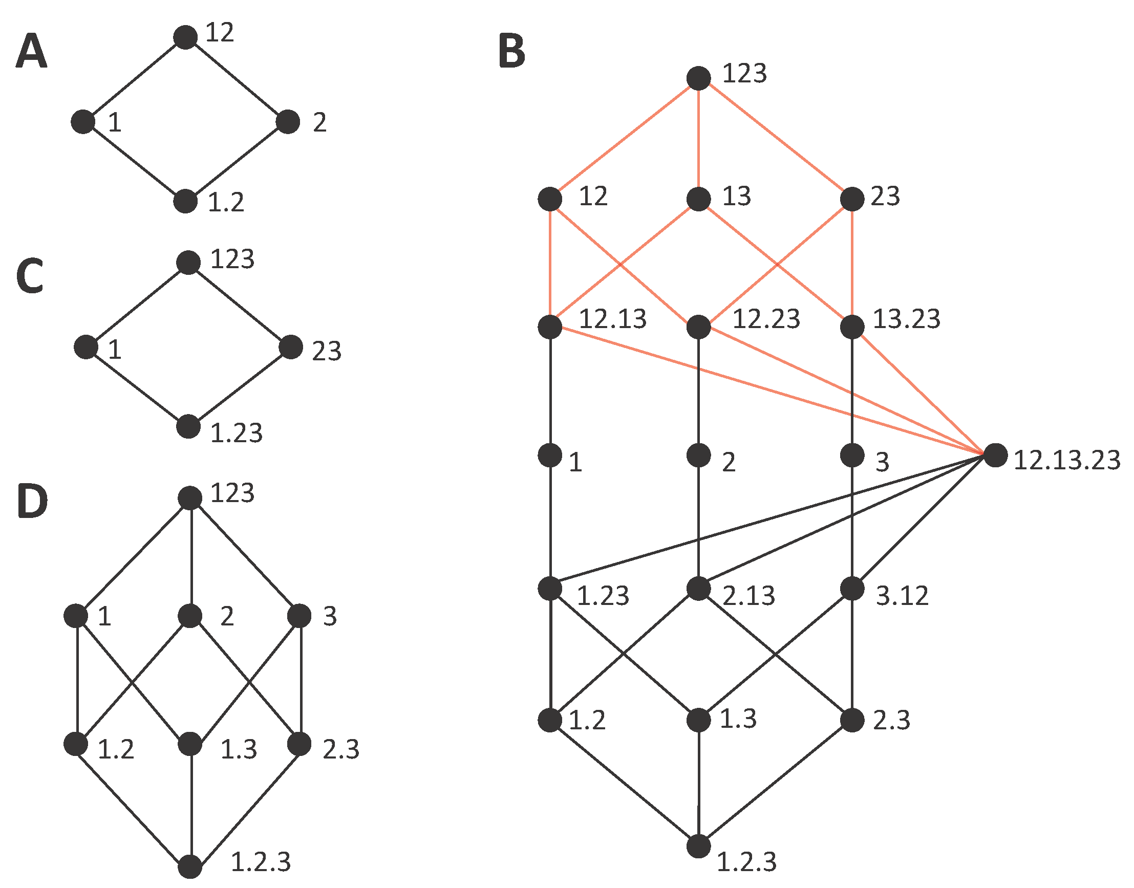
To understand when this is possible, we study how cumulative terms of information loss or gain are mapped from one type of lattice to the other. While in some cases it seems possible to establish a connection between the components of a pair composed by an information gain and an information loss lattice, in other cases the lack of a match is immediately evident. Consider the examples of Figure 6. In Figure 6A,C we reconsider the information gain lattices of Figure 4C,D, which we examined in Section 3.3 to illustrate that we arrive to an inconsistency when trying to extract the bottom cumulative term from the directly calculable mutual informations of 1 and 23 and the same definition of synergy. Figure 4B,D show information loss lattices candidates to be the dual lattice of these gain lattices, respectively, based on the correspondence of the bottom and top collections. While the two information gain lattices only differ from each other in the bottom collection, the information loss lattices are substantially more different, with a different number of nodes. This occurs because, as we discussed above, the concept of a redundancy $1.2.3$ is associated with a loss that is common to removing any of the three variables, considered as the only source of information, and thus, in any candidate dual lattice, a separation of 2 and 3 from the source 23 is required to quantify this redundancy.

The fact that the information gain lattice of Figure 6C and the information loss lattice of Figure 6D have a different number of nodes already indicates that a complete match between their components is not possible. For example, consider the decomposition of $I(S;1)$ in the information gain lattice, as indicated by the nodes comprised in the shaded area in Figure 6C. $I(S;1)$ is decomposed into two incremental terms. To understand which nodes are associated with $I(S;1)$ in the information loss lattice we argue, based on Equation (16)d, that since the node 1 is related to the accumulated loss $L(S;1)=I(S;123)-I(S;1)$, and $L(S;\mathsf{\varnothing })=I(S;123)$, this means that the sum of all the incremental terms which are not in the down set of 1 must correspond to $I(S;1)$. These nodes are indicated by the shaded area in Figure 6D. Clearly, there is no match between the incremental terms of the information gain lattice and of the information loss lattice, since in the former $I(S;1)$ is decomposed into two incremental terms and in the latter is decomposed into four incremental terms. Conversely, for the lattices of Figure 6A,B, the number of incremental terms is the same, which does not preclude from a match.

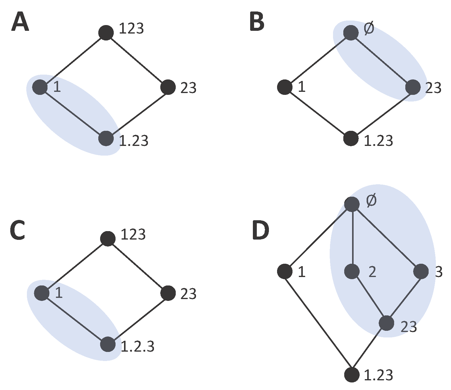
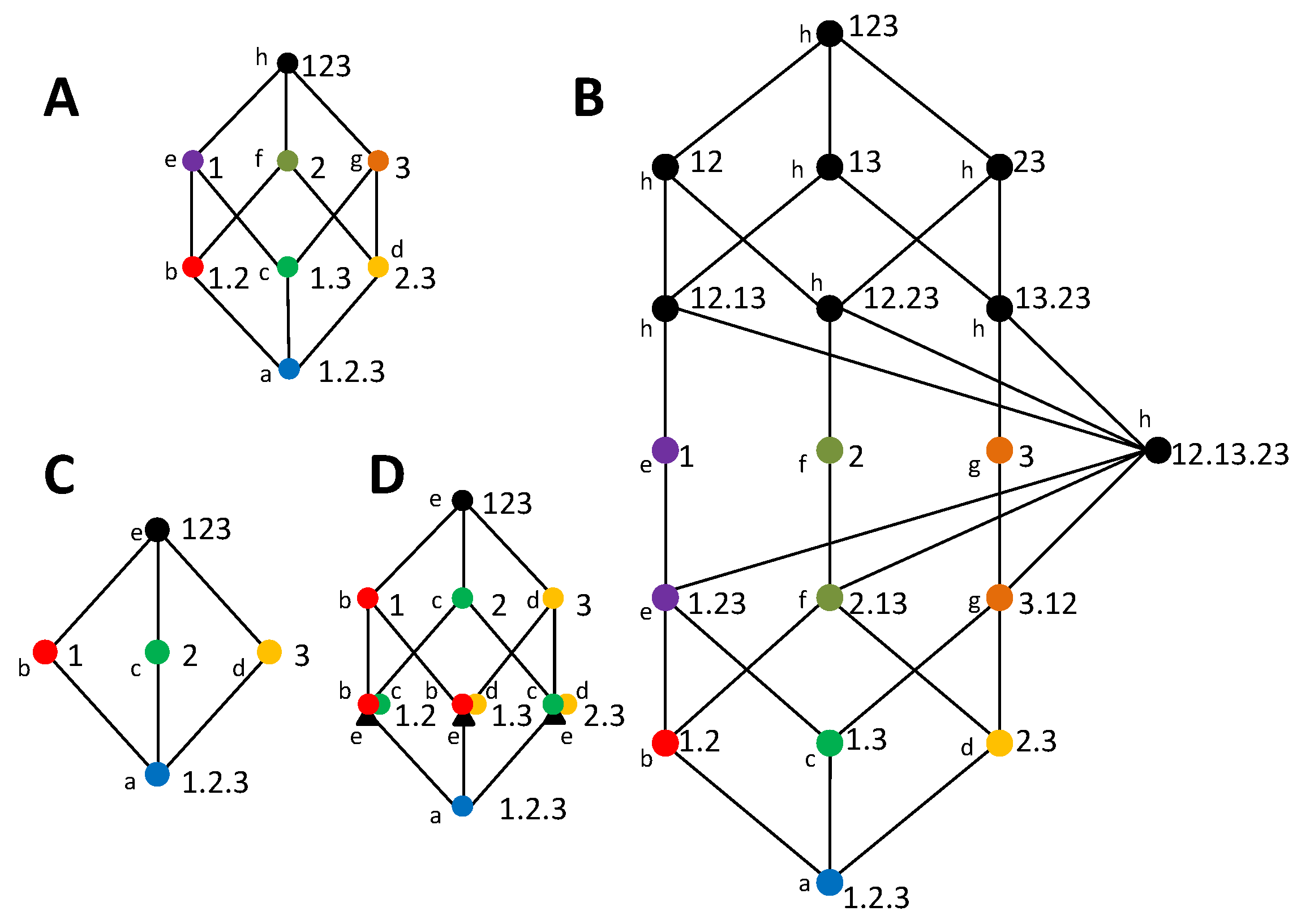
As another example to gain some intuition about the degree to which gain and loss lattices can be connected, we now reexamine the other two lattices of Figure 4. The blue shaded area of Figure 7A indicates the down set of 1, containing all the incremental terms accumulated in $I(S;1)$. The complementary set ${(\downarrow 1)}^C$, indicated by the pink shaded area in Figure 7A, by construction accumulates the remaining information (Equation (16b)), which in this case is $I(S;23|1)$. These two complementary sets of the information gain lattice are mapped to two dual sets in the information loss lattice, as shown in Figure 7B. In Figure 7C, we analogously indicate the sets formed by partitioning the gain lattice given the collection 1, and in Figure 7D the corresponding sets in the information loss lattice. In comparison to the example of Figure 6C,D, for which we have already indicated that there is no correspondence between the gain and loss lattices; here, in neither of the two examples, is this correspondence precluded by the difference in the total number of nodes of the gain and loss lattices. However, in Figure 7C,D, the number of nodes is not preserved in the mapping of the partition sets corresponding to collection 1 from the gain to the loss lattice, which means that the incremental terms cannot be mapped one-to-one from one lattice to the other.

So far, we have examined the correspondence of how collection 1 partitions the total mutual information in different lattices (Figure 6 and Figure 7). This collection is representative of collections α containing a single source, and hence associated with a directly calculable mutual information, e.g., $I(S;1)$. Their corresponding loss in the partition is associated as well with a directly calculable conditional mutual information, e.g., $I(S;23|1)$. Accordingly, we can extend Equation (16b,d) to:

$$\begin{array}{cc}\hfill L(S;\mathbf{A})=I(S;\{\mathbf{R}\left\}\right)-I(S;\mathbf{A})& =\sum _{\beta \in {(\downarrow \mathbf{A})}^C}\Delta I(S;\beta )\hfill \end{array}$$

(17a)

$$\begin{array}{cc}\hfill I(S;{\mathbf{A}}^{\prime })=I(S;\left\{\mathbf{R}\right\})-L(S;{\mathbf{A}}^{\prime })& =\sum _{\beta \in {(\downarrow {\mathbf{A}}^{\prime })}^C}\Delta L(S;\beta ).\hfill \end{array}$$

(17b)

While in Equation (16b), $I(S;\{\mathbf{R}\left\}\right)-I(S;\alpha )$ is a quantification of information loss only within the information gain lattice, the equality in Equation (17a) maps this information loss to the correspondent cumulative term in the information loss lattice. Analogously, Equation (17b) allows mapping a quantification of gain only within the information loss lattice to the cumulative term in the information gain lattice. That is, while Equation (16a,b) only regard the representation of information gain and loss in the gain lattice, and Equation (16c,d) the representation of information gain and loss in the loss lattice, Equation (17) indicates the mapping of the gain and loss representations across lattices, for the single source collections. This mapping was possible for all the pairs of lattices examined, including the ones of Figure 6C,D and Figure 7C,D, which we have shown cannot be dual. This is because Equation (17) only relies on the self-redundancy axiom and the definition of how cumulative and incremental terms are related (Equations (7) and (14)), and hence this mapping can be done between any arbitrary pair of lattices. However, this direct mapping between the two types of lattices does not hold for collections composed by more than one source. For example, consider the mapping of the cumulative term $I(S;1.2)$, composed by the incremental terms indicated by the dashed red ellipse in Figure 7A. Now in the information loss lattice we cannot take the collection $1.2$ to find the corresponding partition, because the role of the collection $1.2$ in the gain and in the loss lattice is different. The collection $1.2$ indicates the redundant information gain with sources 1, 2, and the loss of ignoring other sources apart from 1, 2, respectively.

For dual lattices, since the set of incremental terms has to be the same—so that the mutual information decomposition is unique—this mapping cannot be limited to collections composed by single sources. This means that any collection α of the gain lattice should determine a partition of the incremental terms in the loss lattice that allows retrieving $I(S;\alpha )$, and analogously in the gain lattice to retrieve $L(S;\alpha )$. For example, for the cumulative term $I(S;1.2)$, to identify the appropriate partition in the information loss lattice, we argue that the redundant information between 1 and 2 cannot be contained in the accumulated loss of preserving only 1 or only 2. Accordingly, $I(S;1.2)$ corresponds to the sum of the incremental terms outside the union of the down sets of 1 and 2 in the loss lattice. Following this reasoning, in general:

$$\begin{array}{cc}\hfill I(S;\alpha )& =\sum _{\beta \in {({\displaystyle \bigcup _{\mathbf{B}\in \alpha }}\downarrow \mathbf{B})}^C}\Delta L(S;\beta ),\hfill \end{array}$$

(18a)

$$\begin{array}{cc}\hfill L(S;{\alpha }^{\prime })& =\sum _{\beta \in {({\displaystyle \bigcup _{\mathbf{B}\in {\alpha }^{\prime }}}\downarrow \mathbf{B})}^C}\Delta I(S;\beta ),\hfill \end{array}$$

(18b)

where the same argument led to relate $L(S;{\alpha }^{\prime })$ to gain incremental terms. These equations reduce to Equation (17) for collections with a single source. In Figure 7B, we indicate with the dashed red ellipse the mapping determined by Equation (18a) for $I(S;1.2)$. We can now compare how the cumulative terms $I(S;\alpha )$ are obtained as a sum of incremental terms in the gain and loss lattice, respectively. In the gain lattice, incremental terms are accumulated in $\downarrow \alpha$, descending from α (Equation (7)). In the loss lattice, they are accumulated in a set defined by complementarity to the union of descending sets, which means that these terms can be reached ascending the loss lattice (Equation (18a)). However, this does not imply that all incremental terms decomposing $I(S;\alpha )$ can be obtained ascending from a single node. This can be seen comparing the set of collections related to $I(S;1)$ (blue shaded area) in the information loss lattices of Figure 7B,D. In Figure 7B, this set corresponds to $\uparrow 2.3$, while in Figure 7D there is no β such that the set corresponds to $\uparrow \beta$, and the incremental terms can only be reached ascending from 2 and 3 separately. However, in order for the decomposition to be unique, the set of incremental terms has to be equal in both dual lattices, and thus Equations (7) and (18a) should be equivalent. The same holds for the cumulative terms $L(S;\alpha )$ and Equation (14) and (18b). Furthermore, plugging Equation (18a,b) in Equations (8b) and (15b), respectively, we obtain equations relating the incremental terms of the two lattices:

$$\begin{array}{cc}\hfill \Delta I(S;\alpha )& =\sum _{\beta \in {({\displaystyle \bigcup _{\mathbf{B}\in \alpha }}\downarrow \mathbf{B})}^C}\Delta L(S;\beta )-\sum _{k=1}^{|{\alpha }^{-}|}{(-1)}^{k-1}\sum _{\begin{array}{c}\mathcal{B}\subseteq {\alpha }^{-}\\ \left|\mathcal{B}\right|=k\end{array}}\sum _{\beta \in {({\displaystyle \bigcup _{\mathbf{B}\in \bigwedge \mathcal{B}}}\downarrow \mathbf{B})}^C}\Delta L(S;\beta )\hfill \end{array}$$

(19a)

$$\begin{array}{cc}\hfill \Delta L(S;{\alpha }^{\prime })& =\sum _{\beta \in {({\displaystyle \bigcup _{\mathbf{B}\in {\alpha }^{\prime }}}\downarrow \mathbf{B})}^C}\Delta I(S;\beta )-\sum _{k=1}^{|{\alpha }^{\prime -}|}{(-1)}^{k-1}\sum _{\begin{array}{c}\mathcal{B}\subseteq {\alpha }^{\prime -}\\ \left|\mathcal{B}\right|=k\end{array}}\sum _{\beta \in {({\displaystyle \bigcup _{\mathbf{B}\in \bigwedge \mathcal{B}}}\downarrow \mathbf{B})}^C}\Delta I(S;\beta ).\hfill \end{array}$$

(19b)

If the lattices paired are dual, the right hand side of Equation (19a) has to simplify to a single incremental term $\Delta L(S;\beta )$, and similarly the right hand side of Equation (19b) has to simplify to a single incremental term $\Delta I(S;\beta )$. Taking these constraints into account, we define duality between information gain and loss lattices imposing this one-to-one mapping of the incremental terms:

Lattice duality:

An information gain lattice associated with a set $\mathcal{C}$ and an information loss lattice associated with a set ${\mathcal{C}}^{\prime }$, built according to the ordering relations of Equations (6) and (13), and fulfilling the constraints of Equations (7), (8), (14) and (15), are dual if and only if

$$\begin{array}{cc}& \forall \alpha \in \mathcal{C}\exists \beta \in {\mathcal{C}}^{\prime }:\Delta I(S;\alpha )=\Delta L(S;\beta ),\hfill \end{array}$$

(20a)

$$\begin{array}{cc}& \forall \alpha \in \mathcal{C}\exists \beta \in {\mathcal{C}}^{\prime }:I(S;\alpha )=\sum _{\gamma \in \downarrow \alpha }\Delta I(S;\gamma )=\sum _{\gamma \in \uparrow \beta }\Delta L(S;\gamma ),\hfill \end{array}$$

(20b)

$$\begin{array}{cc}& \forall {\alpha }^{\prime }\in {\mathcal{C}}^{\prime }\exists {\beta }^{\prime }\in \mathcal{C}:\Delta L(S;{\alpha }^{\prime })=\Delta I(S;{\beta }^{\prime }),\hfill \end{array}$$

(20c)

$$\begin{array}{cc}& \forall {\alpha }^{\prime }\in {\mathcal{C}}^{\prime }\exists {\beta }^{\prime }\in \mathcal{C}:L(S;{\alpha }^{\prime })=\sum _{\gamma \in \downarrow {\alpha }^{\prime }}\Delta L(S;\gamma )=\sum _{\gamma \in \uparrow {\beta }^{\prime }}\Delta I(S;\gamma ).\hfill \end{array}$$

(20d)

Equation (20a,c) ensure that the set of incremental terms is the same for both lattices, so that the mutual information decomposition is unique. Equation (20b,d) ensure that the mapping between lattices of Equation (18) is consistent with the intrinsic relation of cumulative and incremental terms within each lattice, introducing a symmetry between the descending and ascending paths of the lattices. This definition does not provide a procedure to construct the dual information loss lattice from an information gain lattice, or vice-versa. However, we have found and we here conjecture that a necessary condition for two lattices to be dual is that they contain the same collections except $\left\{\mathbf{R}\right\}$ at the top of the gain lattice being replaced by ∅ at the loss lattice. This is not a sufficient condition, as can be seen from the counterexample of Figure 7C,D. Importantly, the lattices constructed from the full domain of collections, $\mathcal{A}\left\{\mathbf{R}\right\}$ for the gain and ${\mathcal{A}}^{*}\left\{\mathbf{R}\right\}$ for the loss, are dual. This is because the gain and loss full lattices both contain all possible incremental terms differentiating the different contributions for a certain number of variables n. For lattices constructed from a subset of the collections, the way their incremental terms can be expressed as a sum of different incremental terms of the full lattice (Section 3.1) gives us an intuition of why not all the lattices have their dual pair. In particular, the combination of incremental terms of the full lattice in the incremental terms of a smaller lattice can be specific for each type of lattice, and this causes that, in general, the resulting incremental terms of the smaller lattice can no longer fulfill the constraint connecting incremental and cumulative terms in the other type of lattice. However, duality is not restricted to full lattices. In Figure 8, we show an example of dual lattices, the pair already discussed in Figure 7A,B. We detail all the cumulative and incremental terms in these lattices. While the cumulative terms are specific to each lattice, the incremental terms, in agreement with Equation (20a,c), are common to both. In more detail, the incremental terms are mapped from one lattice to the other by an up/down and right/left reversal of the lattice. From these two reversals, the right/left is purely circumstantial, a consequence of our choice to locate the collections common to both lattices in the same location (for example, to have the collections ordered 1, 2, 3 in both lattices instead of 3, 2, 1 for one of them). Oppositely, the up/down reversal is inherent to the duality between the lattices and reflects the relation between the summation in down sets or up sets in the summands of Equation (20b,d).

To provide a concrete example of information gain and information loss dual decompositions, we here adopted and extended to the multivariate case the bivariate synergy measure defined in [24].

Table 1. Components of the mutual information dual decompositions of Figure 8 based on the synergy measure defined in [24]. Note that we here build this decomposition for exemplary purpose and we do not study the degree to which these measures fulfill other axioms proposed for a proper decomposition.

Term	Measure
$\Delta (S;i.j.k)=I(S;i.j.k)$	$\begin{array}{c}\underset{i.j.k}{\min }I(S;ijk)-\underset{i.j}{\min }I(S;j|i)-\underset{i.k}{\min }I(S;i|k)-\underset{j.k}{\min }I(S;k|j)\end{array}$
$\Delta (S;i.j\backslash k)$	$\begin{array}{c}\underset{i.k}{\min }I(S;ijk)+\underset{j.k}{\min }I(S;ijk)-\underset{i.j.k}{\min }I(S;ijk)-I(S;k)\end{array}$
$\Delta (S;i\backslash j,k)$	$\underset{i.j.k}{\min }I(S;ijk)-\underset{j.k}{\min }I(S;ijk)$
$\Delta (S;ijk\backslash i,j,k)=L(S;i.j.k)$	$I(S;ijk)-\underset{i.j.k}{\min }I(S;ijk)$
$I(S;i.j)$	$I(S;j)-\underset{i.j}{\min }I(S;j|i)$
$L(S;i.j)$	$I(S;ijk)-\underset{i.j}{\min }I(S;ijk)$
$L(S;i)$	$I(S;jk|i)$

lists all the resulting expressions when the extension of this measure is used to determine all the terms in both decompositions. This measure is extended in a straightforward way to the multivariate case, and in particular for the trivariate case defines $L(S;i.j)$ and $L(S;i.j.k)$. The bivariate redundancy measure also already used in [24] corresponds to $I(S;i.j)$. The rest of incremental terms can be obtained from the information loss lattice using Equation (15). Note that we could have proceeded in a similar way starting from a definition of the cumulative terms in the gain lattice, such as $I_{min}$, and then determining the terms of the loss lattice. Here, we use this concrete decomposition only as an example and it is out of the scope of this work to characterize the properties of the resulting terms. Alternatively, we focus on discussing the properties related with the duality of the decompositions.

Most importantly, the dual lattices provide a self-consistent quantification of synergy and redundancy. Equation (20a,c), together with the fact that the bottom incremental terms of lattices are also cumulative terms, ensure that, combining different dual lattices of different order n and composed by different subsets, as studied in Section 3.1, all incremental terms correspond to a bottom cumulative term of a certain lattice. For example, for the lattices of Figure 8, the bottom cumulative term in the information gain lattice, the redundancy $I(S;i.j.k)$, is equal to the top incremental term of the loss lattice, $\Delta (S;i.j.k)$. Similarly, in the bottom cumulative term of the loss lattice, the synergy $L(S;i.j.k)$, is equal to the top incremental term of the gain lattice $\Delta (S;ijk\backslash i,j,k)$.

For dual lattices, the iterative procedure of Section 3.3 can be applied to recover the components of the information gain lattice from a definition of synergy and the components calculated in this way are equal to the ones obtained from the mapping of incremental terms from one lattice to the other. In more detail, let us refer to the bottom and top terms by ⊥ and ⊤, respectively, and distinguish between generic terms such as $I(S;\alpha )$ and a specific measure assigned to it, $\overline{I}(S;\alpha )$. One can define the synergistic top incremental term of the gain lattice using the measure assigned to the bottom cumulative term of the loss lattice, imposing $\Delta I(S;\mathsf{\top })\equiv \overline{L}(S;\mathsf{\perp })$ and self-consistency ensures that the measures obtained with the iterative procedure fulfill $\overline{I}(S;\mathsf{\perp })=\Delta \overline{L}(S;\mathsf{\top })$. Similarly, self-consistency ensures that, if one takes as a definition of redundancy for the cumulative terms of the gain lattice the measure assigned to the incremental terms of the loss lattice based on a definition of synergy, consistent incremental terms are obtained in the gain lattice. That is, $I(S;\mathsf{\perp })\equiv \Delta \overline{L}(S;\mathsf{\top })$ results in $\Delta \overline{I}(S;\mathsf{\top })=\overline{L}(S;\mathsf{\perp })$. It can be checked that these self-consistency properties do not hold in general, for example for the lattices of Figure 7C,D. The properties of dual lattices guarantee that, within the class of dual lattices connected by the decomposition-invariance of cumulative terms, inconsistencies of the type discussed in Section 3.3 do not occur because all lattices share the same correspondence between incremental terms and measures, and all the terms in the decompositions are not decomposition-dependent.

As a last point, the existence of dual information gain and loss lattices, with redundancy measures and synergy measures playing an interchanged role, also indicates, by contrast, that unique information has a qualitatively different role in this type of mutual information decompositions. The measures of unique information always correspond to incremental terms and cannot be taken as the cumulative terms to build the decomposition because they are intrinsically asymmetric in the way different sources determine the measure, which contradicts the symmetry axiom required to connect collections in the lattice to cumulative terms. Despite this difference, the iterative hierarchical procedure of Section 3.3 provides a way to build the mutual information decomposition from a unique information measure, and duality ensures that the decomposition is self-consistent with alternatively having built the decomposition using the resulting redundancy or synergy measures as the cumulative terms of the gain and loss lattice, respectively.

6. Discussion

In this work, we extended the framework of [21] focusing on the lattices that underpin the mutual information decompositions. We started generalizing the type of information gain lattices introduced by [21]. By considering more generally which information gain lattices can be constructed (Section 3.1), we reexamined the constraints that [21] identified for the lattices’ components (Equation (5)) and ordering relation (Equation (6)). These constraints were motivated by the link of each node in the lattice with a measure of accumulated information. We argued that it is necessary to check the validity of each specific lattice given each specific set of variables and that this checking can overcome the problems found by [26] with the original lattices described in [21] for the multivariate case. In particular, we showed that the existence of nonnegative components in the presence of deterministic relations between the variables is directly a consequence of the non-compliance of the validity constraints. This indicates that valid multivariate lattices are not a priori incompatible with a mutual information nonnegative decomposition.

For our generalized set of information gain lattices, we examined the relations between the terms in different lattices (Section 3.1). We pointed out that the two types of information-theoretic quantities associated with the lattices have different invariance properties: The cumulative terms of the information gain lattices are invariant across decompositions, while the incremental terms are decomposition-dependent and are only connected across lattices through the relations resulting from the invariance of the cumulative terms. This produces a qualitative difference in the properties of the redundancy components of the decompositions, which are associated with cumulative terms in the information gain lattices, and the unique or synergy components, which correspond to incremental terms. This difference has practical consequences when trying to construct a mutual information decomposition from a measure of redundancy or a measure of synergy or unique information, respectively. In the former case, as described in [21], the terms of the decomposition can be derived straightforwardly given that the redundancy measure identifies the cumulative terms. In the latter, for the multivariate case, it is not straightforward to construct the decomposition because the synergy or uniqueness measures only allow identifying specific incremental terms. Exploiting the connection between different lattices that results from the invariance of the cumulative terms, we proposed an iterative hierarchical procedure to generally construct information gain multivariate decompositions from a measure of synergy or unique information (Section 3.3). To our knowledge, there was currently no method to build multivariate decompositions from these types of measures and thus this procedure allows application to the multivariate case measures of synergy [23] or unique information [24] for which associated decompositions had only been constructed for the bivariate case. However, the application of this procedure led us to recognize inconsistencies in the determination of decompositions components across lattices. We argued that these inconsistencies are a consequence of the intrinsic decomposition-dependence of incremental terms, to which synergy and unique information components are associated in the information gain lattices. We explained these inconsistencies based on how the components of the full lattice are mapped to components of smaller lattices and indicated that this mapping should be considered to determine if the conceptual meaning of a synergy or unique information measure is compatible with the assignment of the measure to a certain incremental term. With a compatible assignment of measures to incremental terms, the iterative hierarchical procedure provides a consistent way to build multivariate decompositions.

We then introduced an alternative decomposition of the mutual information based on information loss lattices (Section 4). The role of redundancy and synergy components is exchanged in the loss lattices with respect to the gain lattices, with the ones associated with the cumulative terms now being the synergy components. We defined the information loss lattices analogously to the gain lattices, determining validity constraints for the components and introducing an ordering relation to construct the lattices. Cumulative and incremental terms are related in the same way as in the gain lattices, establishing the connection between the lattice and the mutual information decomposition. This type of lattices allows the ready determination of the information decomposition from a definition of synergy. Furthermore, the information loss lattices can be useful in relation to other alternative information decompositions [33,34,35].

The existence of different procedures to construct mutual information decompositions, using a redundancy or synergy measure to directly define the cumulative terms of the information gain or loss lattice, respectively, or using the iterative hierarchical procedure to indirectly determine cumulative terms, raised the question of how consistent are the decompositions obtained from these different methods. Therefore, we studied, in general, the correspondence between information gain and information loss lattices. The final contribution of this work was the definition of dual gain and loss lattices (Section 5). Within a dual pair, the gain and loss lattices share the incremental terms, which can be mapped one-to-one from the nodes of one lattice to the other. Duality ensures self-consistency, so that the redundancy components obtained from a synergy definition are the same as the synergy components obtained from the corresponding redundancy definition. Accordingly, for dual lattices, any of the procedures can be equivalently used, leading to a unique mutual information decomposition compatible with the existence of unique notions of redundancy, synergy, and unique information. Nonetheless, each type of lattice expresses in a more transparent way different aspects of the decomposition, and allows different components to be extracted more easily, and thus may be preferable depending on the analysis.

As in the original work of [21] that we aimed to extend, we have here considered generic variables, without making any assumption about their nature and relations. However, a case which deserves special attention is that of variables associated with time-series, so that information decompositions allow the study of the dynamic dependencies in the system [36,37]. Practical examples include the study of multiple-site recordings of the time course of neural activity at different brain locations, with the aim of understanding how information is processed across neural systems [38]. In such cases of time-series variables, a widely-used type of mutual information decomposition aims to separate the contribution to the information of different causal interactions between the subsystems, e.g., [39,40]. Consideration of synergistic effects is also important when trying to characterize the causal relations [41]. In fact, when causality is analyzed by quantifying statistical predictability using conditional mutual information, a link between these other decompositions and the one of [21] can be readily established [42,43].

The proposal of [21] has proven to be a fruitful conceptual framework and connections to other approaches to study information in multivariate systems have been explored [44,45,46]. However, despite subsequent attempts, e.g., [22,23,24,25], it is still an open question how to decompose in multivariate systems the mutual information into nonnegative contributions that can be interpreted as synergy, redundancy, or unique components. This issue constitutes the main challenge that limits so far the practical applicability of the framework. Another challenge for this type of decomposition is to be able to further relate the terms in the decomposition with a functional description of the parts composing the system [10]. In this direction, an attractive extension could be to adapt the decompositions to an interventional approach [10,47], instead of one based on statistical predictability. This could allow one to better understand how the different components of the mutual information decomposition are determined by the mechanisms producing dependencies in the system. In practice, this would help, for example, to dissect information transmission in neural circuits during behavior, which can be done by combining the analysis of time-series recordings of neural activity using information decompositions with space-time resolved interventional approaches based on brain perturbation techniques such as optogenetics [10,48,49]. This interventional approach could be incorporated to the framework by adopting interventional information-theoretic measures suited to quantify causal effects [50,51,52].

Overall, this work provides a wider perspective to the ground constituents of the mutual information decompositions introduced by [21], introduces new types of lattices, and helps to clarify the relation between synergy and redundancy measures with the lattice’s components. The consolidation of this theoretical framework is expected to foster future applications. An advance of this work of practical importance is that it describes how to build mutual information multivariate decompositions from redundancy, synergy, or unique information measures and shows that different procedures are consistent, leading to a unique decomposition when dual information gain and information loss lattices are used.

References

1. Timme, N.; Alford, W.; Flecker, B.; Beggs, J.M. Synergy, redundancy, and multivariate information measures: An experimentalist’s perspective. J. Comput. Neurosci. 2014, 36, 119–140. [Google Scholar] [CrossRef] [PubMed]
2. Anastassiou, D. Computational analysis of the synergy among multiple interacting genes. Mol. Syst. Biol. 2007, 3, 83. [Google Scholar] [CrossRef] [PubMed]
3. Lüdtke, N.; Panzeri, S.; Brown, M.; Broomhead, D.; Montemurro, M.; Kell, D. Information-theoretic Sensitivity Analysis: A general method for credit assignment in complex networks. J. R. Soc. Interface 2008, 19, 223–235. [Google Scholar] [CrossRef] [PubMed]
4. Watkinson, J.; Liang, K.; Wang, X.; Zheng, T.; Anastassiou, D. Inference of regulatory gene interactions from expression data using three-way mutual information. Ann. N. Y. Acad. Sci. 2009, 1158, 302–313. [Google Scholar] [CrossRef] [PubMed]
5. Oizumi, M.; Albantakis, L.; Tononi, G. From the phenomenology to the mechanisms of consciousness: Integrated information theory 3.0. PLoS Comput. Biol. 2014, 10, e1003588. [Google Scholar] [CrossRef] [PubMed]
6. Faes, L.; Marinazzo, D.; Nollo, G.; Porta, A. An Information-Theoretic Framework to Map the Spatiotemporal Dynamics of the Scalp Electroencephalogram. IEEE Trans. Biomed. Eng. 2016, 63, 2488–2496. [Google Scholar] [CrossRef] [PubMed]
7. Averbeck, B.B.; Latham, P.E.; Pouget, A. Neural correlations, population coding and computation. Nat. Rev. Neurosci. 2006, 7, 358–366. [Google Scholar] [CrossRef] [PubMed]
8. Panzeri, S.; Macke, J.; Gross, J.; Kayser, C. Neural population coding: Combining insights from microscopic and mass signals. Trends Cogn. Sci. 2015, 19, 162–172. [Google Scholar] [CrossRef] [PubMed]
9. Haefner, R.; Gerwinn, S.; Macke, J.; Bethge, M. Inferring decoding strategies from choice probabilities in the presence of correlated variability. Nat. Neurosci. 2013, 16, 235–242. [Google Scholar] [CrossRef] [PubMed]
10. Panzeri, S.; Harvey, C.D.; Piasini, E.; Latham, P.E.; Fellin, T. Cracking the neural code for sensory perception by combining statistics, intervention, and behavior. Neuron 2017, 93, 491–507. [Google Scholar] [CrossRef] [PubMed]
11. Wibral, M.; Vicente, R.; Lizier, J.T. Directed Information Measures in Neuroscience; Springer: Berlin/Heidelberg, Germany, 2014. [Google Scholar]
12. Panzeri, S.; Schultz, S.; Treves, A.; Rolls, E.T. Correlations and the encoding of information in the nervous system. Proc. Biol. Sci. 1999, 266, 1001–1012. [Google Scholar] [CrossRef] [PubMed]
13. Pola, G.; Thiele, A.; Hoffmann, K.P.; Panzeri, S. An exact method to quantify the information transmitted by different mechanisms of correlational coding. Netw. Comput. Neural Syst. 2003, 14, 35–60. [Google Scholar] [CrossRef]
14. Amari, S. Information geometry on hierarchy of probability distributions. IEEE Trans. Inf. Theory 2001, 47, 1701–1711. [Google Scholar] [CrossRef]
15. Ince, R.A.A.; Senatore, R.; Arabzadeh, E.; Montani, F.; Diamond, M.E.; Panzeri, S. Information-theoretic methods for studying population codes. Neural Netw. 2010, 23, 713–727. [Google Scholar] [CrossRef] [PubMed]
16. Latham, P.E.; Nirenberg, S. Synergy, Redundancy, and Independence in Population Codes, Revisited. J. Neurosci. 2005, 25, 5195–5206. [Google Scholar] [CrossRef] [PubMed]
17. Chicharro, D. A Causal Perspective on the Analysis of Signal and Noise Correlations and Their Role in Population Coding. Neural Comput. 2014, 26, 999–1054. [Google Scholar] [CrossRef] [PubMed]
18. Schneidman, E.; Bialek, W.; Berry, M.J. Synergy, redundancy, and independence in population codes. J. Neurosci. 2003, 23, 11539–11553. [Google Scholar] [PubMed]
19. McGill, W.J. Multivariate information transmission. Psychometrika 1954, 19, 97–116. [Google Scholar] [CrossRef]
20. Bell, A.J. The co-information lattice. In Proceedings of the 4th international Symposium on Independent Component Analysis and Blind Source Separation, Nara, Japan, 1–4 April 2003; pp. 921–926.
21. Williams, P.L.; Beer, R.D. Nonnegative Decomposition of Multivariate Information. arXiv 2010. [Google Scholar]
22. Harder, M.; Salge, C.; Polani, D. Bivariate measure of redundant information. Phys. Rev. E 2013, 87, 012130. [Google Scholar] [CrossRef] [PubMed]
23. Griffith, V.; Koch, C. Quantifying synergistic mutual information. arXiv 2013. [Google Scholar]
24. Bertschinger, N.; Rauh, J.; Olbrich, E.; Jost, J.; Ay, N. Quantifying unique information. Entropy 2014, 16, 2161–2183. [Google Scholar] [CrossRef]
25. Ince, R.A.A. Measuring multivariate redundant information with pointwise common change in surprisal. arxiv 2016. [Google Scholar]
26. Rauh, J.; Bertschinger, N.; Olbrich, E.; Jost, J. Reconsidering unique information: Towards a multivariate information decomposition. In Proceedings of the 2014 IEEE International Symposium on Information Theory, Honolulu, HI, USA, 29 June–4 July 2014; pp. 2232–2236.
27. Williams, P.L. Information Dynamics: Its Theory and Application to Embodied Cognitive Systems. Ph.D. Thesis, Indiana University, Bloomington, IN, USA, 2011. [Google Scholar]
28. Griffith, V.; Chong, E.K.P.; James, R.G.; Ellison, C.J.; Crutchfield, J.P. Intersection Information based on Common Randomness. Entropy 2014, 16, 1985–2000. [Google Scholar] [CrossRef]
29. Bertschinger, N.; Rauh, J.; Olbrich, E.; Jost, J. Shared Information—New Insights and Problems in Decomposing Information in Complex Systems. In Proceedings of the European Conference on Complex Systems 2012; Springer: Cham, Switzerland, 2013; pp. 251–269. [Google Scholar]
30. Barrett, A. Exploration of synergistic and redundant information sharing in static and dynamical Gaussian systems. Phys. Rev. E 2015, 91, 052802. [Google Scholar] [CrossRef] [PubMed]
31. Cover, T.M.; Thomas, J.A. Elements of Information Theory, 2nd ed.; Wiley: Hoboken, NJ, USA, 2006. [Google Scholar]
32. Ince, R.A.A. The Partial Entropy Decomposition: Decomposing multivariate entropy and mutual information via pointwise common surprisal. arxiv 2017. [Google Scholar]
33. Olbrich, E.; Bertschinger, N.; Rauh, J. Information decomposition and synergy. Entropy 2015, 17, 3501–3517. [Google Scholar] [CrossRef]
34. Perrone, P.; Ay, N. Hierarchical quantification of synergy in channels. arXiv 2016. [Google Scholar]
35. Schneidman, E.; Still, S.; Berry, M.J.; Bialek, W. Network information and connected correlations. Phys. Rev. Lett. 2003, 91, 238701. [Google Scholar] [CrossRef] [PubMed]
36. Chicharro, D.; Ledberg, A. Framework to study dynamic dependencies in networks of interacting processes. Phys. Rev. E 2012, 86, 041901. [Google Scholar] [CrossRef] [PubMed]
37. Faes, L.; Kugiumtzis, D.; Nollo, G.; Jurysta, F.; Marinazzo, D. Estimating the decomposition of predictive information in multivariate systems. Phys. Rev. E 2015, 91, 032904. [Google Scholar] [CrossRef] [PubMed]
38. Valdes-Sosa, P.; Roebroeck, A.; Daunizeau, J.; Friston, K. Effective connectivity: Influence, causality and biophysical modeling. Neuroimage 2011, 58, 339–361. [Google Scholar] [CrossRef] [PubMed]
39. Solo, V. On causality and Mutual information. In Proceedings of the 47th IEEE Conference on Decision and Control, Cancun, Mexico, 9–11 December 2008; pp. 4639–4944.
40. Chicharro, D. On the spectral formulation of Granger causality. Biol. Cybern. 2011, 105, 331–347. [Google Scholar] [CrossRef] [PubMed]
41. Stramaglia, S.; Cortes, J.M.; Marinazzo, D. Synergy and redundancy in the Granger causal analysis of dynamical networks. New J. Phys. 2014, 16, 105003. [Google Scholar] [CrossRef]
42. Williams, P.L.; Beer, R.D. Generalized Measures of Information Transfer. arXiv 2011. [Google Scholar]
43. Lizier, J.; Flecker, B.; Williams, P. Towards a synergy-based approach to measuring information modification. In Proceedings of the IEEE Symposium on Artificial Life, Singapore, 16–19 April 2013; pp. 43–51.
44. Wibral, M.; Priesemann, V.; Kay, J.W.; Lizier, J.T.; Phillips, W.A. Partial information decomposition as a unified approach to the specification of neural goal functions. Brain Cogn. 2017, 112, 25–38. [Google Scholar] [CrossRef] [PubMed]
45. Banerjee, P.K.; Griffith, V. Synergy, redundancy, and common information. arXiv 2015. [Google Scholar]
46. James, R.G.; Crutchfield, J.P. Multivariate Dependence Beyond Shannon Information. arXiv 2016. [Google Scholar]
47. Chicharro, D.; Panzeri, S. Algorithms of causal inference for the analysis of effective connectivity among brain regions. Front. Neuroinform. 2014, 8, 64. [Google Scholar] [CrossRef] [PubMed]
48. O’Connor, D.H.; Hires, S.A.; Guo, Z.; Li, N.; Yu, J.; Sun, Q.Q.; Huber, D.; Svoboda, K. Neural coding during active somatosensation revealed using illusory touch. Nat. Neurosci. 2013, 16, 958–965. [Google Scholar] [CrossRef] [PubMed]
49. Otchy, T.; Wolff, S.; Rhee, J.; Pehlevan, C.; Kawai, R.; Kempf, A.; Gobes, S.; Olveczky, B. Acute off-target effects of neural circuit manipulations. Nature 2015, 528, 358–363. [Google Scholar] [CrossRef] [PubMed]
50. Ay, N.; Polani, D. Information flows in causal networks. Adv. Complex Syst. 2008, 11, 17–41. [Google Scholar] [CrossRef]
51. Lizier, J.T.; Prokopenko, M. Differentiating information transfer and causal effect. Eur. Phys. J. B. 2010, 73, 605–615. [Google Scholar] [CrossRef]
52. Chicharro, D.; Ledberg, A. When Two Become One: The Limits of Causality Analysis of Brain Dynamics. PLoS ONE 2012, 7, e32466. [Google Scholar] [CrossRef] [PubMed]
Figure 1. Information gain decompositions of different orders and for different subsets of collections of sources. (A,B) Lattices constructed from the complete domain of collections as defined by Equation (5) for n = 2 and n = 3 , respectively. Pale red edges in (B) identify the embedded lattice formed by collections that do not contain univariate sources. (C) Alternative decomposition based only on sources 1 and 23. (D) Alternative decomposition that does not contain bivariate sources.
Entropy 19 00071 g001
Figure 2. Mapping between the incremental terms of the bivariate lattice for 1, 2 and the full trivariate lattice for 1, 2, 3. (A) The bivariate lattice with each node marked with a different color (and also, redundantly, with a different lower case letter, for no-color printing). (B) The trivariate lattice with the nodes coloured consistently with the mapping to the bivariate lattice. In more detail, the incremental term of each node of the bivariate lattice is obtained as the sum of the incremental terms of the nodes of the trivariate lattice with the same color.
Entropy 19 00071 g002
Figure 3. Mapping of the incremental terms of the full lattice to lattices formed by subsets of collections (A) The lattice of Figure 1D with each node marked with a different color (and also a different lower case letter, for no-color printing). (B) The trivariate lattice with the nodes coloured consistently with the mapping to the lattice of (A). In more detail, the incremental term of each node of the smaller lattice is obtained as the sum of the incremental terms of the nodes of the trivariate lattice with the same color. (C) Another lattice obtained from a subset of the collections, with each node marked with a different color (and lower case letter). (D) The lattice of (A) now with its nodes coloured consistently with the mapping to the lattice of (C). In contrast to the mapping between (B) and (A), here each incremental term of (D) can contribute to more than one incremental term of (C), with a positive (circle) or negative (triangles) contribution.
Entropy 19 00071 g003
Figure 4. Examples of information gain lattices that result in inconsistencies when trying to derive redundancy terms from a synergy definition, as explained in Section 3.3.
Entropy 19 00071 g004
Figure 5. Information loss decompositions of different orders and for different subsets of collections of sources. (AD) The lattices are analogous to the information gain lattices of Figure 1. Note that the lattice embedded in (B), indicated with the pale red edges, corresponds to the one shown in (D), differently than in Figure 1.
Entropy 19 00071 g005
Figure 6. The correspondence between information gain and information loss lattices. (A,C) Examples of information gain lattices. (B,D) Information loss lattices candidates to be their dual lattices, respectively. The shaded areas comprise the collections corresponding to incremental terms that contribute to I ( S ; 1 ) in each lattice.
Entropy 19 00071 g006
Figure 7. Correspondence between information gain and information loss lattices. (A,C) Examples of information gain lattices. (B,D) Information loss lattices candidates to be their dual lattice, respectively. The blue shaded areas comprise the collections corresponding to incremental terms that contribute to I ( S ; 1 ) in each lattice. The pink shaded areas surrounded with a dotted line comprise the collections corresponding to incremental terms that contribute to the complementary information I ( S ; 23 | 1 ) in each lattice. In (A,B), the dashed red lines encircle the incremental terms contributing to I ( S ; 1 . 2 ) .
Entropy 19 00071 g007
Figure 8. Dual trivariate decompositions for the sets of collections that do not contain bivariate sources. (A) Information gain lattice. (B) Information loss lattice. In each node together with the collection, the corresponding cumulative and incremental terms are indicated. Note that the incremental terms are common to both lattices and can be mapped by reversing the lattice up/down and right/left. In the information loss lattice, the cumulative terms of collections containing single sources, L ( S ; i ) , i = 1 , 2 , 3 , are directly expressed as the corresponding conditional information.
Entropy 19 00071 g008