1. Introduction
Spatial-temporal pattern structures are ubiquitous [
1,
2], especially in biological and human phenomena [
3,
4,
5,
6]. They commonly originate from (nonlinear) driving forces acting locally on the elements of a spatially-extended system. Often, this type of global emergent behavior cannot be “guessed” simply from a direct qualitative inspection of the interactions between the individual constituents (i.e., at the microscopic level). The full dynamics, the macroscopic description [
6], can be understood only as a collective effect. Such a scenario frames what is frequently termed in the literature complex systems.
Likewise, phase transitions do constitute an extremely relevant class of processes. In particular, the so-called critical phenomena lead to a very rich range of distinct comportment [
7,
8]. Briefly, not too close to a critical point
, the system microscopic organization varies continuously with a given control parameter
λ (for instance, temperature, chemical potential, etc.), maintaining a certain main characteristic, e.g., a non-null magnetization or some degree of ordered aggregation, quantified by a macroscopic order parameter Γ. However, by crossing
(with
usually vanishing), the system qualitatively changes, going through a phase transition, e.g., becoming non-magnetic or complete disordered. Moreover, around the critical point [
7], there is the development of infinite correlation lengths and the rise of universal features (like detail-independent critical exponents). A non-trivial association between complexity and criticality is generally believed to exist [
9].
The wide purpose of Cellular Automata (CA) (the acronym CA will mean either Cellular Automaton or its plural form Cellular Automata; which one is actually being used should be clear from each sentence’s specific context) models [
10,
11] couples very well with the idea of emergent complexity. From a pure computational (algorithmic) point of view, CA is an extremely versatile framework: in principle CA would be able to realize an universal Turing machine [
12,
13,
14], hence to perform complete general information processing. Thus, putting aside the controversial discussion if CA could (or not) describe any natural process [
15], the fact is that CA are extremely useful in simulating distinct complex systems [
16]. For example, the quite hard task of mimicking life and/or live organisms (individually or collectively) was the initial motivation for John von Neumann, with the help of Stanislaw Ulam, to propose CA in the 1940s, an approach reborn in the 1970s, in part due to the general interest in the John H. Conway’s “Game of Life” CA. Nowadays, CA have become a frequently employed theoretical tool in biological and ecological studies (refer, e.g., to [
17,
18,
19]).
The key aspects underlying CA can be summarized as the following. Suppose we cross-grade the system pertinent configurational (spatial, phase, etc.) space, portraying it in terms of cells (or elements). Then, to each cell
, we can ascribe a state variable
(function of a discrete time
), whose numerical (usually also discrete) values indicate, say, particles’ density, pigment color, action states (active/inactive, life/death, infected/non-infected), energy content, etc. As the system dynamically evolves [
20], the set
may give rise to intricate tile-like arrangements. This can be so even though at the elements’ level, the local responses to the interactions are simple. In this way, the full CA behavior reflects global complexity [
21].
Due to the CA inherent discrete formulation, contrary to the already mentioned close connection between CA and complex systems, it may be much more difficult to establish an appropriate link between deterministic CA and phase transitions. This is particularly true with respect to continuous transitions, i.e., critical phenomena (for probabilistic CA, phase transitions are more easily observed; see, for instance, [
22,
23]). Actually, in most CA constructions, there are no “good”
λ’s, which could play the role of control parameters (eventually, they might exist, but then demanding certain restrictions to act as such, like requiring the number of possible states
S to be very high [
24]).
Recently, a deterministic CA with a new ingredient, inertia, has been proposed [
25]. The original goal in [
25] was to find a minimal, not dedicated model capable of describing the basic aspects of ecotones [
26,
27,
28]: zones between geographic regions of distinct biomes. In such transition areas, there is the coexistence of groups of species coming from different ecosystems. In many concrete situations, it is still not completely understood how less fitted (e.g., to the nearby biomes conditions) exogenous animals and plants can survive [
29,
30]. They eventually would perish in a more homogeneous environment if competing with the same stronger (better adapted) local endogenic species [
31,
32]. To address the problem, some of us have introduced an intrinsic (in opposition to certain probabilistic proposals in the literature; see, e.g., [
33,
34,
35]) resistance, the inertia
I, to the system’s natural rules of evolution [
25]. As a consequence, depending on
(which assumes discrete values), it becomes more difficult for the interactions to change the state
of each cell
n. By playing with the initial conditions and the
distribution, it is possible to generate spatial patterns of meta-communities qualitatively similar to those in ecotones [
21,
26,
27,
28].
In the present contribution, we shall explore CA with inertia in very general terms, showing that I can act as a proper control parameter. Considering analysis procedures typical from statistical physics, we study the evolution of ensembles of CA with different random initial configurations. We thus are able to characterize average properties for the CA final spatial patterns’ structures, clearly identifying behavior similar to phase transitions. Although, because of their discrete nature, CA cannot lead to “true” critical phenomena, certain features of usual continuous phase transitions can be observed as we change . In fact, by assuming different distribution of inertia values among the CA cells, we observe distinct and intricate heterogeneities in the emergence of spatial patterns. Intriguingly, for certain quantities, we even can see indications of discontinuous phase transitions. These apparent contradictory results eventually can be explained in terms of the finite character of the CA model and the discreteness of the inertia parameter I. Along the work, potential applications for our model are also briefly mentioned. Finally, in the last discussion and conclusion section, we make final considerations about the rise of phase transitions in CA and the important role, in this regard, represented by inertia-like quantities (using ecotones as an illustration).
2. The Model: CA with Inertia
2.1. Basic Definitions
In our CA construction, the space is represented by a square lattice of N × N elements (or cells). At the discrete time t (), the state of cell (hereafter labeled n ()) is given by , whose possible numerical values are , 0 and +1. We assume that only cells in the (active) states and have the eventual power of altering the S’s of their neighbors. Therefore, the state 0 is neutral in terms of any competition dynamics. We consider a further internal parameter associated with each cell n, , which is an integer between zero and eight. We call such a quantity “inertia” since it characterizes the cells’ intrinsic resistance to changes in their actual state values. In the more general case, could be a function of time, but for our purposes, here, we restrict the analysis only to time-independent I’s.
At time
t, let us define
, with
the population of the state
in the neighborhood of
n. The cell
n has
contiguous neighbors if it is, respectively, in the bulk, border or corner of the square lattice (we are supposing hard wall boundary conditions (HWBD)). This is known as Moore’s neighborhood of radius one. We assume HWBD because many systems that potentially can be described by our model (like the already mentioned ecotones landscape, as well as fragmentation patterns in ecosystems [
36]) require limited boundaries as their spatial arena. The time evolution of each
follows from two deterministic rules:
- (i)
The inertial rule: If the dynamical rule below is applied, otherwise , i.e., the state of n remains unchanged.
- (ii)
The dynamical rule: , with sign the signal of x.
Two aspects of (i)–(ii) should be highlighted. First, any neighbor of n in the state 0 does not contribute to make , a necessary condition to change (if , the dynamical rule (ii) is not applied). Therefore, cells in state 0 cannot modify their neighborhoods. Second, cells in the active state S (either −1 or +1) belonging to the neighborhood of n can alter only if is greater than the cell n resistance to switch (given by the inertia parameter ).
From now on, by ‘one step’ of evolution (), we will mean that we have considered Rules (i)–(ii) for all of the elements in the CA lattice, obtaining the full set from .
To characterize certain system features, we define two groups of quantities calculated at each time
t. The first relates to the population of a state
S, given by
. For our
lattice, the total population is
. The second represents the degree of clusterization of the CA lattice spatial pattern, either of the whole system,
c, or only of the cells in state
S,
. The clusterization measures the amount of “agglomeration” of the CA elements, i.e., the number and size of clusters formed by cells in the same state. For their definition, suppose
the state corresponding to
(obviously, making sense only if there is a unique most populated state). If there is a
, we set
, otherwise
. Then,
and
read:
with:
In Equation (
2),
is the local clusterization around the site
n regardless of the state of
n. On the other hand,
estimates the accumulation of the state
S around a cell
n if such a cell is also in the state
S. These functions have been proven very useful in typifying certain spatial patterns in biology [
25]. However, as we have explicitly verified, the use of other methods (like Hoshen–Kopelman [
37]) to gauge the CA degree of clusterization yields the same qualitative results obtained in the present work.
Finally, we specify a third parameter, τ, representing the the minimal number of full iterations (i.e., the number of time steps; see above) for a specific initial lattice to reach a stationary configuration. In other words, for , the CA remains unchanged for any further application of the evolution rules. As we are going to discuss, only in relatively few cases we will not have a finite τ for the CA initial lattices considered.
2.2. A Statistical Physics-Like Analysis: Averaging over Ensembles of Initial Configurations
Since we shall identify typical properties of the proposed CA, we assume a statistical physics point of view and consider ensembles of initial configurations for the CA lattice. Then, we calculate the quantities described in
Section 2.1 by performing averages over a large number of time evolved lattices (from such ensembles), obtaining “mean characteristics” of the system.
To standardize the analysis, we always take lattices having initially and the same fixed number of elements in the 0 state, with being equal to the integer closest to . Unless otherwise explicitly mentioned, we set (a value already large enough to illustrate the CA main aspects and also allowing relatively fast simulations). We commonly generate about lattices (in the numerically harder cases ), resulting in very good means for any situation studied. For (total population and ), we discuss two distinct ensembles of lattices: (a) one where is homogeneously distributed in the range ; and (b) another in which the clusterization is homogeneously distributed in the interval . (we observe that such an interval, appropriate for our purposes here, is consistent with (but hard to meet for ), also allowing one to generate a large number of replicas for each value).
Observing these restrictions, the spatial distribution of initial states in the cells is random.
We mention that comparatively few initial CA lattices either are not able to converge to a final stationary structure or may take a too long time to do so. Thus, from all of the initial lattices created, we have used only those with
(typically corresponding to 97%–99% of
). In the
Appendix A, we give simple examples of end patterns that are not stationary because they oscillate between very similar (but not the same) configurations.
Our procedure is therefore: (a) to dynamically evolve each replica in the ensembles according to Rules (i)–(ii) until achieving a steady condition, and then; (b) to perform the pertinent averages over the resulting CA configurations.
3. Results
In
Section 3, we use the following notational convention. Since any
will be a constant for
, the final stationary value of
will be denoted simply as
q. Furthermore, any quantity
q should be understood as the resulting average over the corresponding ensemble.
3.1. CA with Zero Inertia
We start by briefly presenting conventional results for a CA without inertia (, ∀ n), the most usual context in the literature. This case will serve as a reference to discuss the behavior of CA with .
First, we note that as expected (so, we do not show any plot for such situation here), the final population and clusterization of elements in the state increase fairly linearly with the initial value of the population, . This linearity comes from the fact that the average distribution of a state S in the neighborhood of a cell n is . If increases, increases accordingly. Since the dynamical “pressure” to change the state of n to an active S goes with , it follows that the final number of elements in state S is basically proportional to .
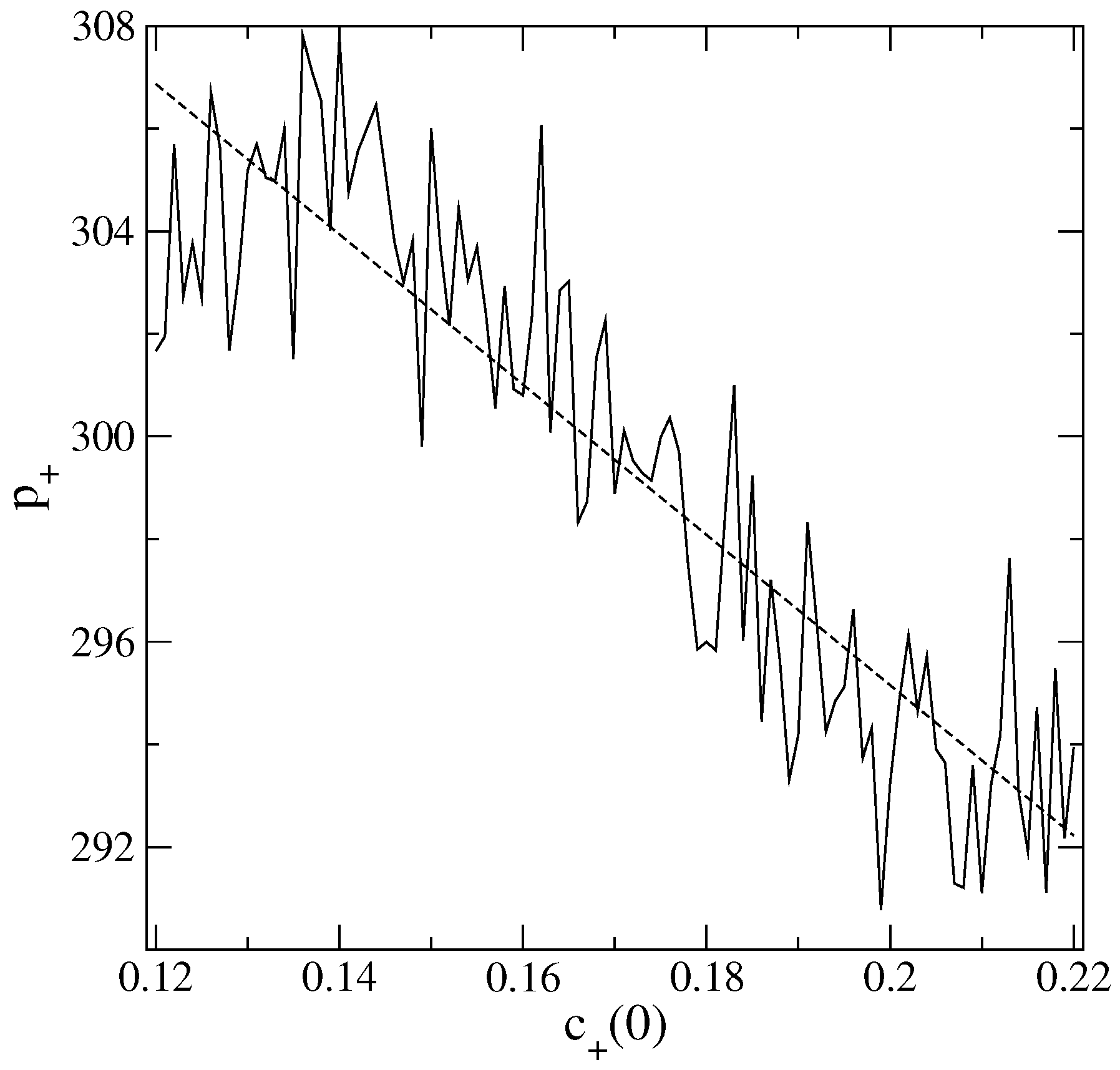
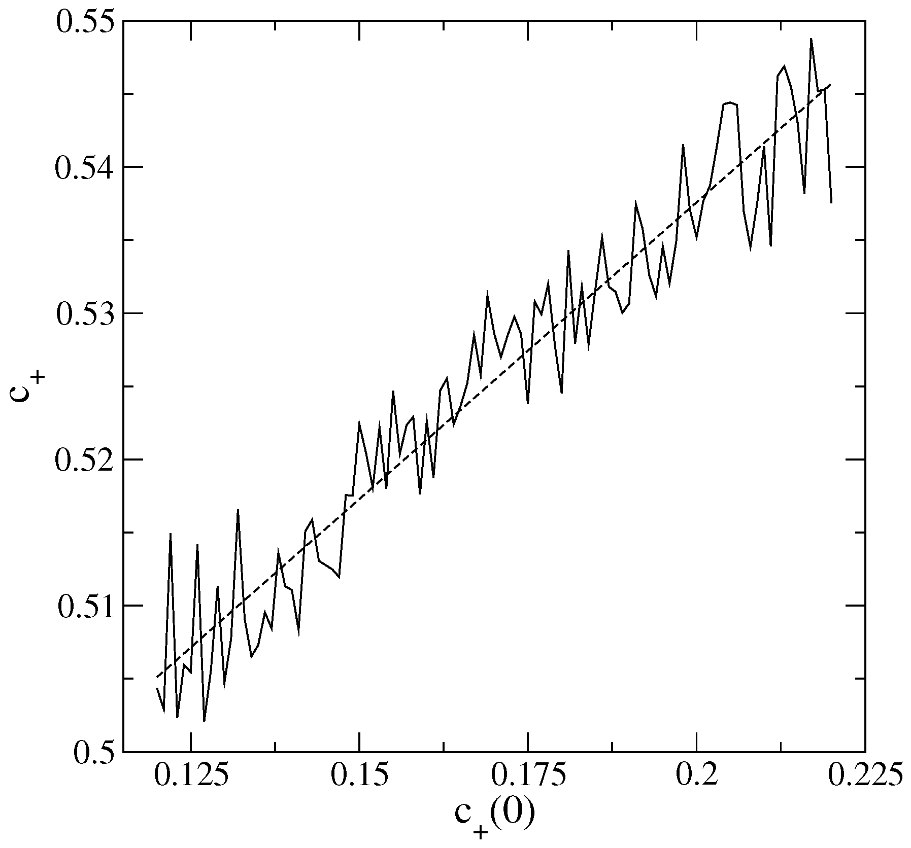
An interesting behavior emerges when we calculate
and
as a function of
. Examples are shown in
Figure 1 and
Figure 2. Observe that both
and
decrease with increasing
, so
plays an inverse role to that of
. This is apparently counter-intuitive: one could expect higher initial agglomerations of an active
S (acting as compact “source” regions at
) to enhance the spread of
S throughout the lattice, leading to a dominance of
S over the other states.
To comprehend the above, it is important to recall that the parameter
, examined alone, in principle gives just the average degree of agglomeration of a particular
S, but not any detailed information about the spatial distribution of the
S cells across the whole lattice. However, the construction of ensembles with the
’s in the range of values used here results only in mild variations of
. Hence, in this case, a higher
necessarily implies that the
cells are more localized in specific regions of the CA lattice. On the opposite, lower
’s yield more uniformly distributed
along it. Thus, around the initially localized
clusters (whose sizes increase and number decreases with an increasing in
), certainly there is a tendency for the growth of
. However, in the remainder of the lattice,
is mostly competing with the neutral state 0, so very quickly,
will dominate. As a consequence, the more concentrated is
originally, the higher the final overall preeminence of
, explaining the trends in
Figure 1 and
Figure 2.
We finish this brief analysis of the case considering how τ changes with and . From simulations, one finds that τ increases with and decreases with (recall that we are assuming an interval for , such that Δ is not too large). Regarding , if originally with both states equally dispersed, rapidly, there will be a situation of equilibrium between them, leading to shorter τ’s. If , typically at the stationary condition (), . Nonetheless, this relative gain of will require slightly longer times to be achieved as moderately increases. On the other hand, high means that the cells are agglomerated in certain regions of the lattice (see the previous discussion). Therefore, quickly, these regions will be populated by and the others by the , resulting in an expeditious convergence to the stationary configuration.
3.2. CA with Homogeneous Inertia
The simplest (homogeneous) case of a CA with inertia is that in which constant ∀ n (). Note that the extreme value leads to no dynamics (i.e., ) once the evolution rules (with ) cannot modify the system, because any cell has at most eight first neighbors.
First, consider
and
in terms of
. Similar to
in
Section 3.1, on average, a rather linear dependence of
on
is observed. Furthermore, as expected, when
, both the magnitude of
, as well as the slopes of the resulting straight lines
decrease steadily with increasing
I. This reflects the natural fact that the cells tend to remain in their initial state for higher
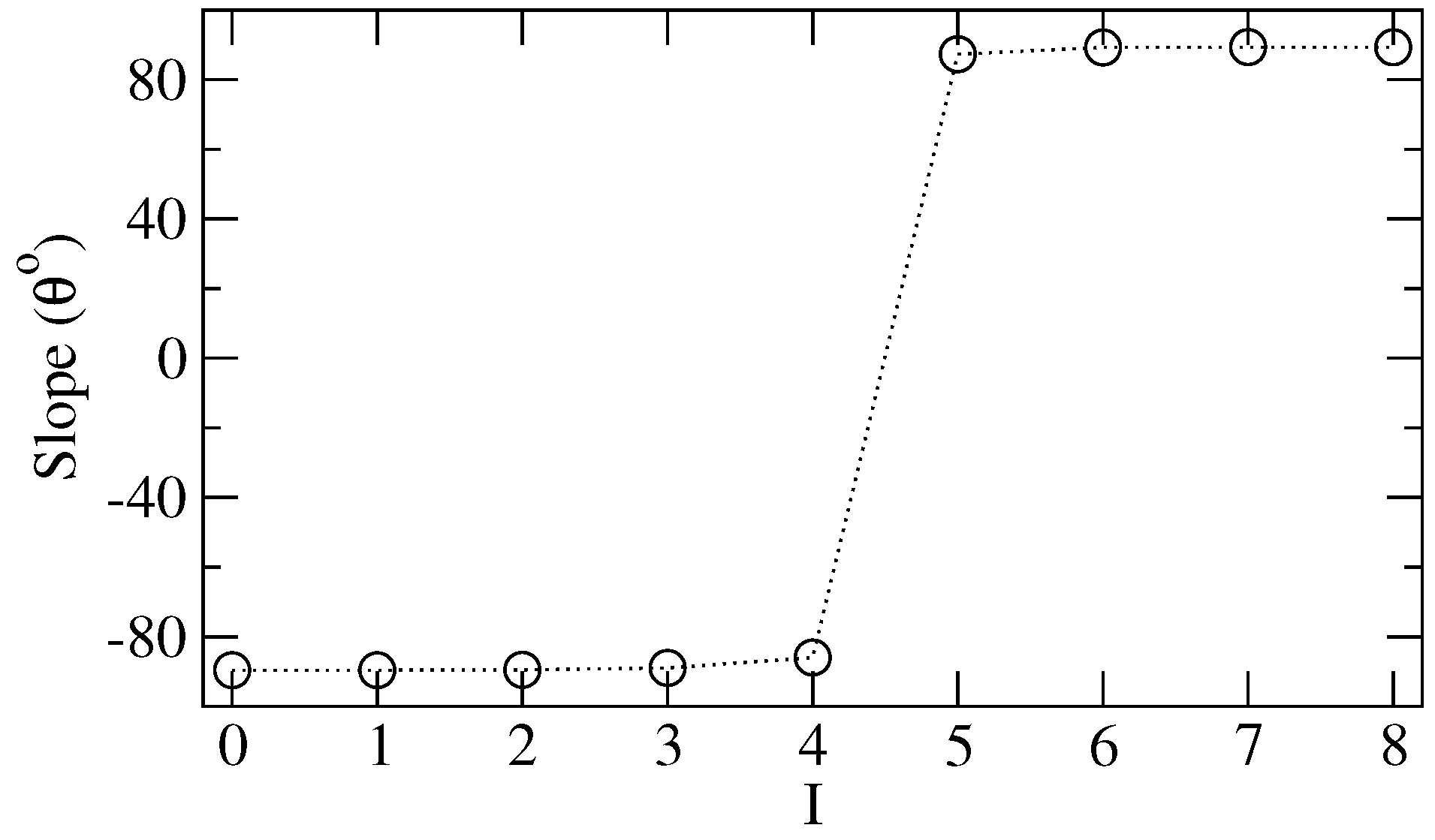
I’s, producing a final pattern, which does not substantially differ from the initial one. Likewise, on average,
displays a linear variation with
. However, differently from
, the angular coefficient of the
straight line does not display a simple monotonic behavior with
I. This is clear in
Figure 3a, where we plot the slope (i.e., the angle
θ (in degrees)) of the straight line
as a function of
I. There is a clear peak for
θ: for
the (positive) correlation between
, and
increases with
I, whereas when
, such a correlation decreases with
I. To understand such a result, which indicates some sort of dynamical transition, we recall that when
, only a neighborhood of
n with
or more cells in the same active
would be able to eventually alter
. Then, as
I grows, the system evolution becomes more sensitive to the initial population because high values of
(and, consequently, larger
state concentrations) are fundamental to trigger state changes. Nevertheless, when
and if
is not overwhelming,
starts to decouple from
since the dynamics passes to be strongly controlled by the cells’ internal resistance, and only huge initial clusterization of
(not the case for
not very large) could significantly modify the CA lattice original configuration.
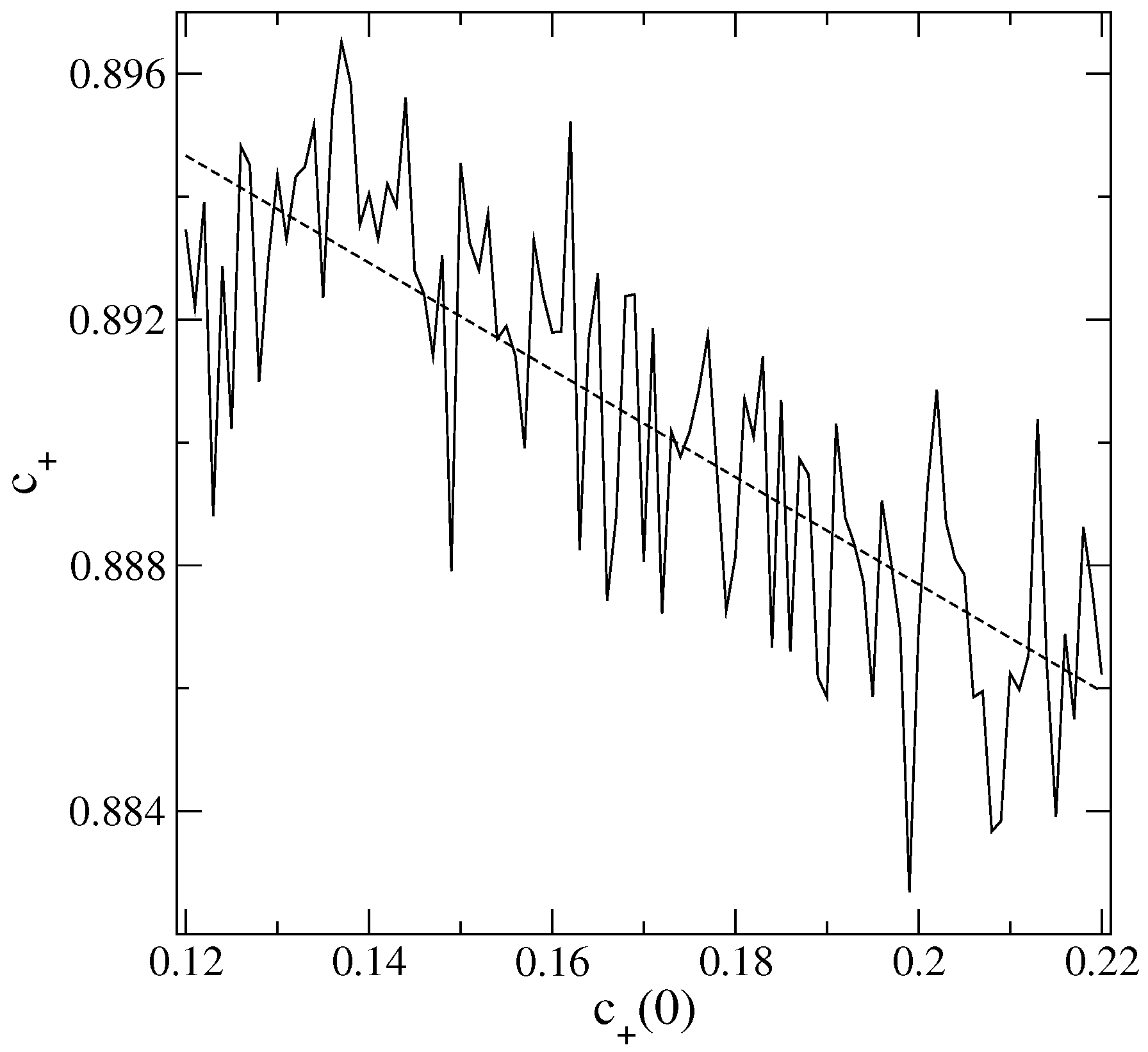
Second, we observe that even stronger evidence of transition is given by the behavior of
versus
. The slopes (again, the corresponding straight lines’ angles
θ) are shown in
Figure 3b. Similarly to the
case in
Section 3.1, for
, one finds that
decreases with increasing
(negative
θ). Therefore, the mechanism relating
with
discussed in
Section 3.1 is still dominant if the inertia is low. However, when
, the final
increases with
. Indeed, then, only very aggregated
’s around a cell
n (of high inertia) will have the ability to modify
. Further, in such a context of greater
I’s, the more randomly-distributed population of
’s across the lattice barely will increase (contrasting with the dynamics of the equivalent situation, but with
in
Section 3.1).
Third, regarding
, for the
, interval,
displays only a weak dependence on
, with the magnitude of
slightly decreasing as
I increases (see the explanation in
Section 3.1). For
, the cells’ enhanced resistance induces a stronger correlation between
and
, so that higher final will demand higher initial clusterizations. This is so because for large inertia, changes in a given
are possible only if
n is in the vicinity of a large cluster of the active
S. As a consequence, an active state
S will spread out only if “supported” by already existing clusters of
S.
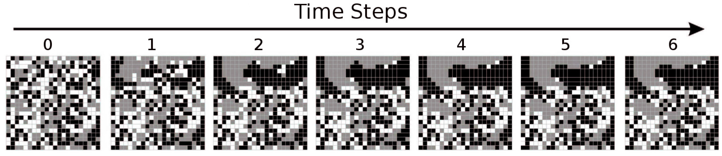
Lastly, the cells tend to remain in their original states as the inertia grows. Therefore, the number of accessible intermediary configurations until stationarity usually reduces with
I, shortening
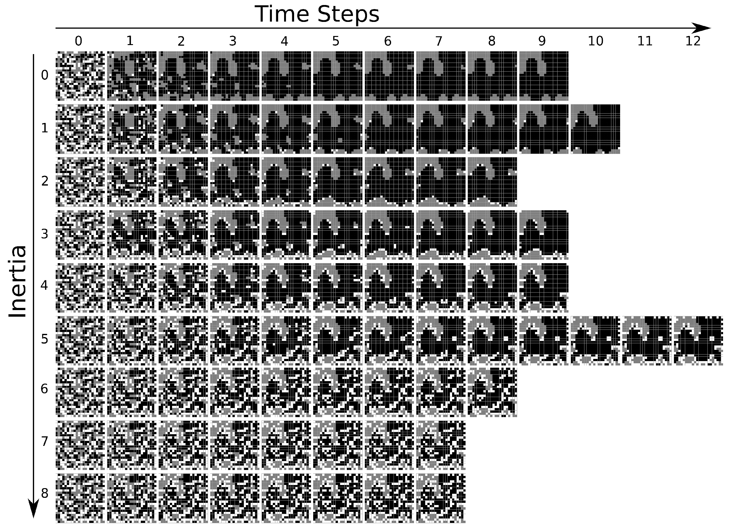
τ. As an illustration, in
Figure 4, we show a typical CA evolution. We consider the same initial lattice, for which
and
and different
I’s. The black, white and grey colors represent, respectively, states
, 0 and
. In this particular example, when
,
iteration steps are necessary to achieve the steady condition. For the other
I’s, we have:
for
;
for
; and
for
. In the first six cases, the final CA patterns are all distinct from each other. For
, the initial configuration cannot be changed from the evolution rules.
Some other discussed features of the present CA system can also be identified in
Figure 4. For instance, we see that the final clusterization becomes strongly correlated to the initial clusterization for high
I’s. However, perhaps the most interesting property observed in
Figure 4 is that the number of cells in the neutral (or dynamically passive)
state in the final configuration increases with
I. In this particular example, when
, all the initial 0 elements are transformed into the active
states. However, as
I increases, a fraction of the initial 0 cells are able to survive up to the stationary configuration, with
growing with
I (obviously
for
).
Thus, it is clear that the presence of an internal resistance variable, inertia, is essential for the endurance of states that are dynamically neutral (or somehow “fragile”) during the time evolution. This property has been used to model ecotones (i.e., biome transition regions) in a previous work [
25]. Nonetheless, here, we shall briefly mention a further potential application for our CA formulation. As nicely put in [
38], the phenomenon of frustration is a very common behavior in complex systems, arising when a local minimum of energy cannot be achieved due to opposite force mechanisms. For example, three
-spins located at the vertices of a triangle cannot simultaneously be at the lowest energy level if their mutual interaction is antiferromagnetic. Frustration-induced phase transitions have already been described by CA [
39], but through stochastic implementations (briefly, we define two deterministic set of rules,
and
, and at each time
t, choose probabilistically one of them to be applied to the CA elements). In magnetic lattices displaying frustration, if the coupling extends over larger neighborhoods and the interactions are anisotropic, the system may develop regions of regular ordering, separated by irregular lines of frustrated magnets [
40]. With a proper extension of the rules in
Section 2.1, the evolution of our deterministic CA with inertia can simulate the formation of such regions, where the state 0 could then represent the frustrated magnets (this is presently an ongoing study) (cf., in
Figure 4, see the configurations for
at
and
at
).
3.3. CA with Inertia Following Spatial Patterns
So far, we have discussed the case of the same inertia value for the whole CA lattice. However, one can imagine complete arbitrary distributions of inertia among the CA cells, conceivably leading to very diverse and rich dynamics. Therefore, just to give a flavor of more general possibilities, we next consider three relatively simple illustrative examples, which we call Patterns I, II and III for the inertia spatial distribution.
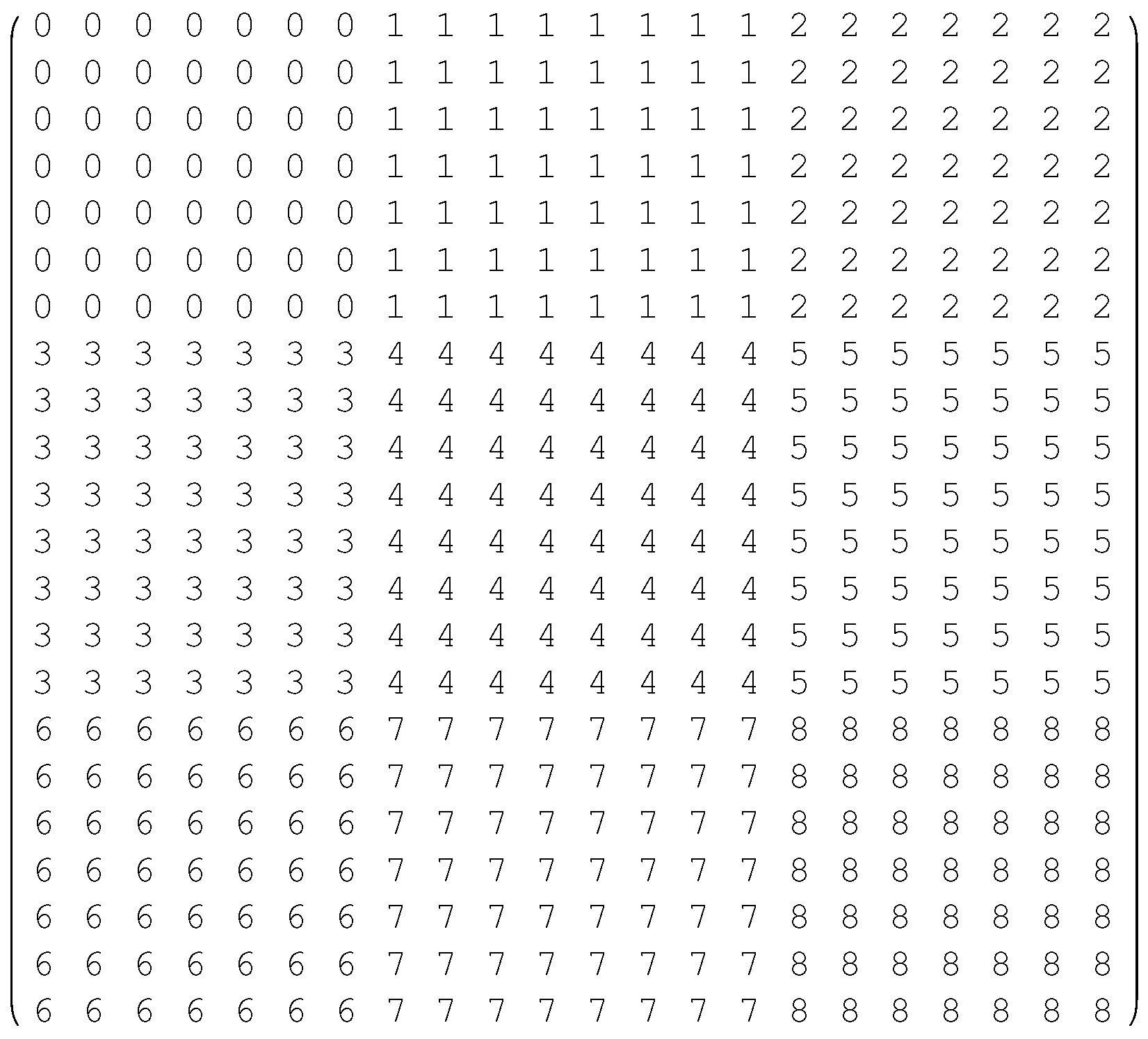
3.3.1. Pattern I: Regional Block Distribution of Inertia
The inertia Pattern I is depicted in
Figure 5. There are in total nine regional blocks of inertia, each having a fixed value of
. Successive adjacent horizontal blocks (from the top-left to the bottom-right) have
I incremented by one unit.
Qualitatively, the dependence of
and
on
is similar to that for homogeneous constant
I’s. There is a linear positive correlation of these quantities with the initial
population, so that
and
grow linearly with
. Furthermore,
decreases with increasing
, which is the trend in
Section 3.2 for
I small. On the other hand,
Figure 6 shows that (up to fluctuations, cf.
Figure 1 and
Figure 2)
tends to increase with
. This is the case in
Section 3.2, but only for greater
I’s. Such results point to an interesting propensity for gradual block-like inertia distributions. The behavior of
is always more strongly determined by the lower
I’s, whereas
as a function of
(
) is more influenced by the higher (lower)
I’s. Regarding
τ, in the ranges considered for the initial conditions, the inertia Pattern I is akin to
, with larger
’s (
’s) giving rise to longer (shorter)
τ’s. Nevertheless, there is an important difference: the average number of iterations is usually lower for Pattern I than for
. This is so because regions with high
I quickly converge to a local stationary configuration, thus slightly decreasing
τ compared to CA without inertia (
Section 3.1).
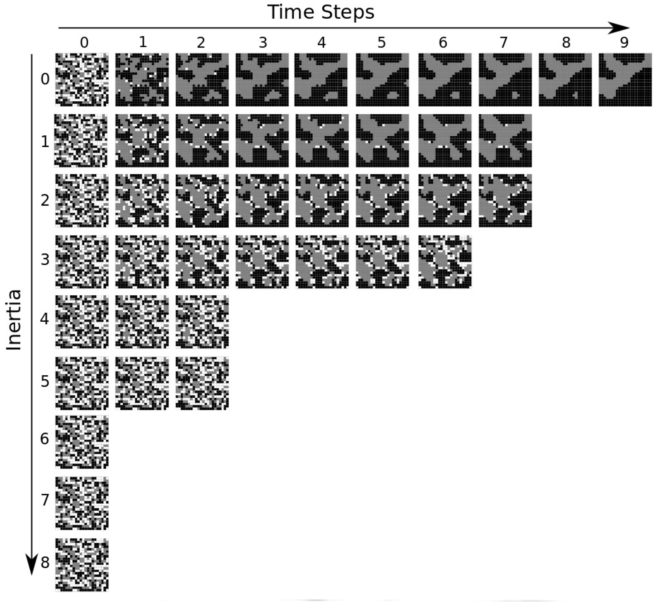
Figure 7 shows a typical time evolution of a CA with the inertia Pattern I (in this example,
). Observe that the cells belonging to blocks with low inertia are able to form clusters of active
states (only very few cells in the 0 state survive). In contrast, elements in the blocks with higher inertia are more evenly distributed among the three possible
S values. In such blocks, there is no prevalence of a major state, and the final
increases as
I (regionally) increases.
CA are very useful to model phase separation processes [
41], e.g., as occurring in binary mixtures [
42]. In this regard, we observe that the blocks in
Figure 7, where
have become very clusterized (for
), could be interpreted as the regions of the final segregated phases. On the other hand, certain lattice areas do not allow a strong domination by a single type of state (say, representing a specific molecule). Therefore, a cluster distribution of inertia acts like a heterogeneous medium for the distinct states (or particles) diffusion, thus engendering complex morphological partition [
43].
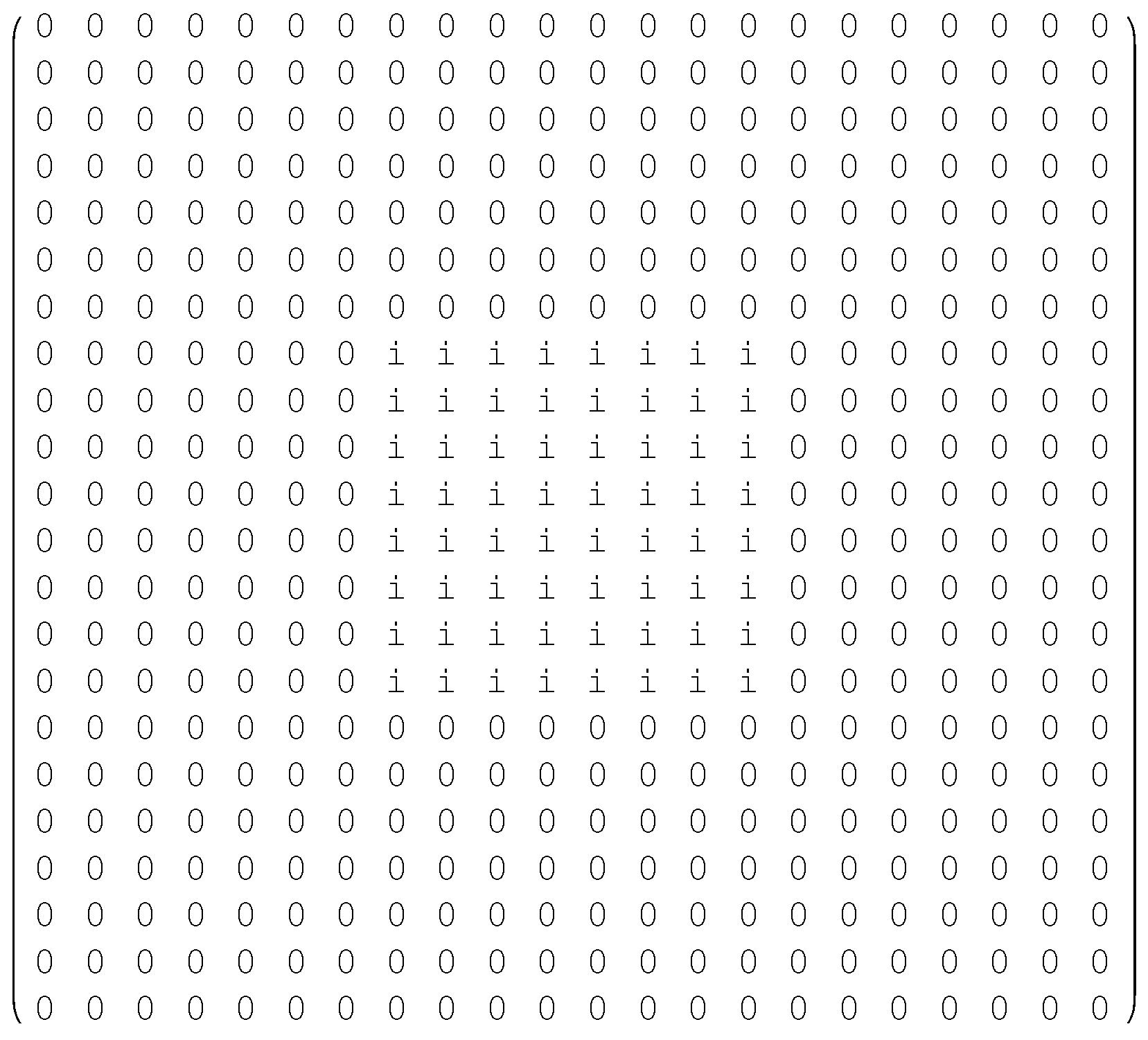
3.3.2. Pattern II: A Unique Central Region with a Non-Null Constant Inertia
The inertia spatial Pattern II is represented in
Figure 8. Just the elements of a central square block
B have non-null inertia (
for any
n in
B and
otherwise). Note that the number of
neighbors to the
B border (corners) cells is three (five). Thus, usually,
would lead to no dynamics for the
B elements in the case of a random distribution of states for the initial CA lattice. Therefore, here, we only assume
.
This kind of inertia pattern is interesting to test how an initial compact group with a certain opposition to changes (but with a random distribution of
S’s) can influence the full system evolution. For applications of CA to problems where there are resistant agents or refractory periods, during which there is no response to external signals from certain elements, see, e.g., models of resistance to market innovations [
33] and rippling arrangements in biological cells [
44].
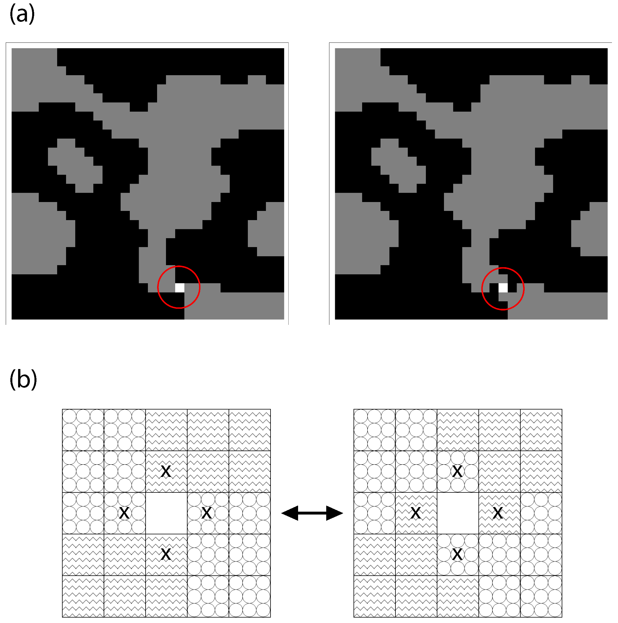
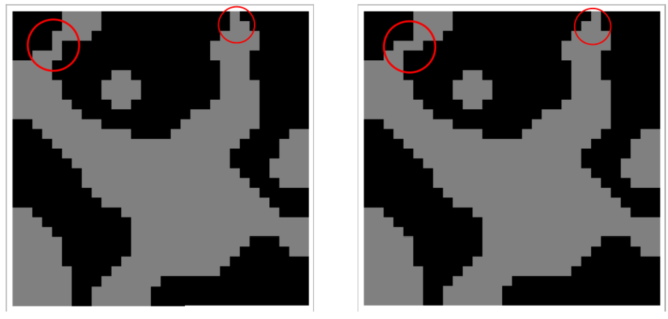
A first distinct feature of Pattern II (with respect to the case of
everywhere, i.e.,
) is that the number of replicas in the ensembles (
Section 2.2), which does not converge to stationarity, slightly decreases (increases) when
(
). It can be understood as the following. For null inertia, there are some lattices that oscillate between few final, similar, but not equal, configurations (
Appendix A). For Pattern II with
, a certain number
of these oscillations are eliminated (see
Appendix A), and the corresponding lattices stabilize. For
(still a low inertia value), unless for these eliminations, other aspects of the CA dynamics are not drastically altered. However, for greater
i’s, the border cells of
B start to act as a contour of fixed
S’s, generating a geometric constraint in the evolution of the remaining lattice cells (especially those in the immediate vicinity of
B). Hence, a given number
of initial lattices will not converge to a steady condition due to the appearance of border oscillating structures (see the discussion in the
Appendix A) around
B. For higher
i’s,
, if
B is big enough, the situation here. As a consequence, compared to
Section 3.1, the average
τ for Pattern II very mildly increases (decreases) if
(
). In fact, for
, the extra lattices (
), which are now included in the calculations, often have their individual
τ’s longer than the average
τ in
Section 3.1. For
, the block
B generally converges more rapidly to a steady configuration, thus lowering the lattices overall
τ.
Qualitatively, the time evolutions of the cells with zero inertia in both Pattern II and
everywhere are akin. Therefore, Pattern II leads to
and
with a fair linear growth with
. Furthermore,
and
decrease with increasing
i, following the same trend of a fixed
I for the whole lattice (
Section 3.2). As for
and
as a function of
, they have the same behavior shown in
Figure 1 and
Figure 2, with the values of
and
decreasing as
i increases.
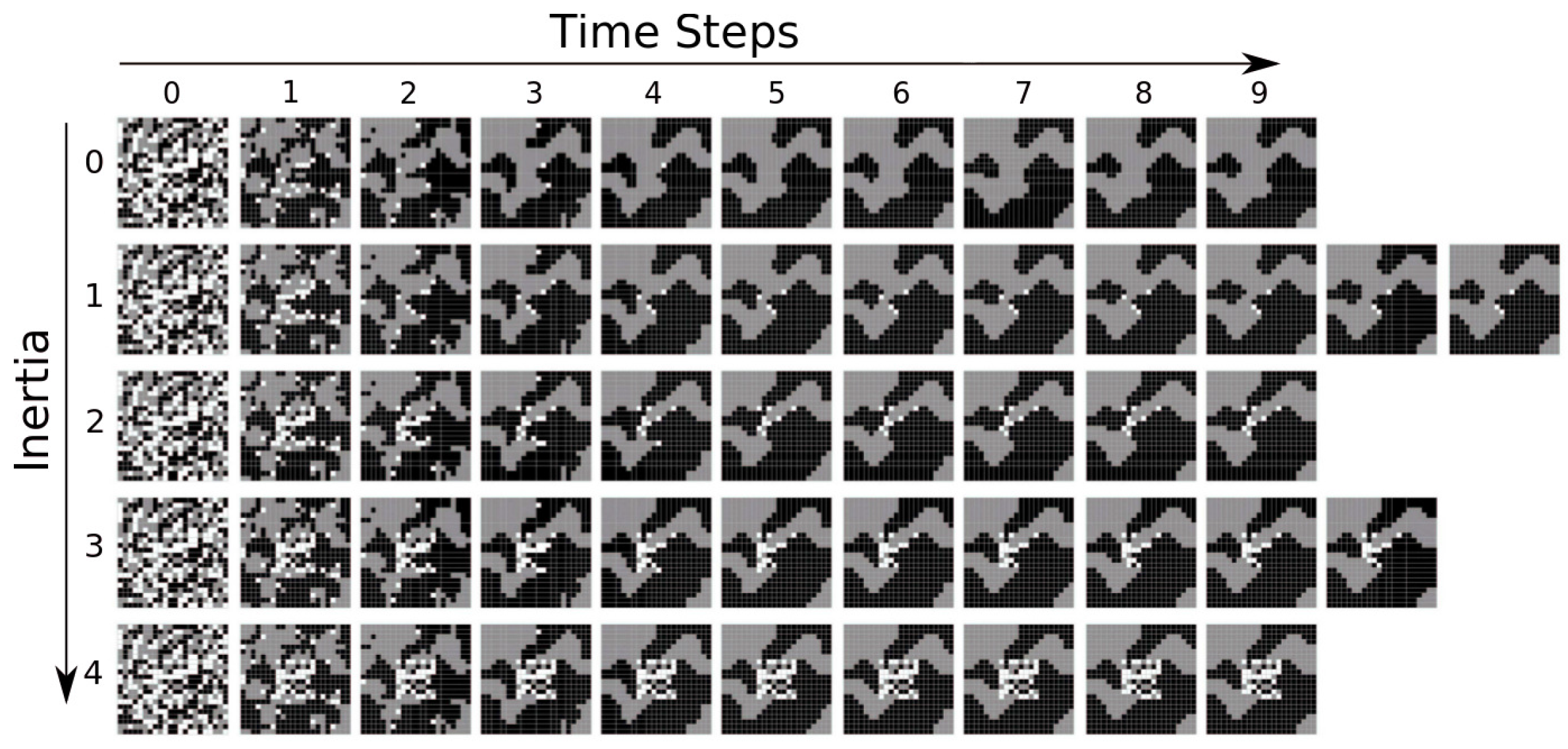
Figure 9 illustrates the dynamics of a specific CA with the inertia Pattern II. Here,
τ is 9, 11, 9, 10, 9, respectively, for
i equal to 0, 1, 2, 3, 4. From the plots, we observe that basically the cells in and around
B are the most affected by the values of
i. The remaining lattice elements evolve following almost the same sequence of configurations seen in the case without inertia (
Figure 9 first row, in which
). These results contrast with previously-mentioned models in the literature [
33,
44], whose resistive elements tend to change the final configuration of the entire system. The main difference is that the initial states of the
B cells (of
) are randomly distributed. Hence, they do not share a common
S (say, a strong opinion about some specific subject), which in the long term could influence the global distribution of states, representing voting intention, language, cultural preferences, etc., and eventually giving rise to phase transition-like phenomena [
45]. Actually, the CA with inertia Pattern II is an appropriate construction to describe systems presenting regions of homogeneous phases coexisting with regions of very heterogeneous structures (cf.,
Figure 9).
3.3.3. Pattern III: Non-Null Inertia Initially Only for the Neutral State
The
state is passive under the evolutionary rules described in
Section 2.1. Hence, it is often completely annihilated by the active states when
everywhere. This is no longer the case if all of the cells have a same non-null inertia (
Section 3.2). However, then one could ask which other inertia distributions can preserve
. The intuitive answer is to assume that only the elements starting in the neutral state can withstand changes. To investigate such situation, we finally consider the inertia Pattern III, where we suppose that initially the cells
n at
(
) have an inertia value
(
).
Here, again,
and
depend linearly on
. The
and
magnitudes strongly decrease with
I, the same trend seen in
Section 3.2. Further, the always positive slopes (the angles
θ) of the straight lines
and
monotonically diminish with
I, however with a very mild variation (especially for
) when
. Hence, contrary to
Figure 3a, the slope
θ of the
curve versus
I does not present a peak, which would characterize a qualitative dynamical change (at least regarding the final
clusterization in terms of
). This distinct behavior from that in
Section 3.2 occurs because initially, only the
cells (so with
) can act like “buffer” elements to prevent the growth of
agglomerations. But dynamically
is a passive state. Therefore, for
I small, the formation of
clusters at the end of the evolution is not so critically dependent on
, as would be the case if the
active state at the beginning had also a non-null inertia.
On the other hand, an important transition is observed when we analyze
versus
. For
(
), the final
decreases (increases) with
. This is illustrated in
Figure 10, where one sees that the slope of
versus
I has the same behavior of
Figure 3b (but notice a different onset). Such similarity indicates that the strongest influence on the final value of
in terms of
is played by the susceptibility of neutral elements to become active
states (a mechanism that depends on
I) and not due to the competition between
and
to transform each other.
For Pattern III, the average τ drops quickly with increasing I. Indeed, as I grows, the cells tend to become “immune” and then excluded from evolution. With a reduced number of elements participating in the dynamics, naturally, the convergence to a stationary configuration is quicker.
A typical evolution is illustrated in
Figure 11. As
I increases,
can survive until the stationary configuration is reached, especially if they are located in the borders that divide clusters of the
and
states (this is just the mechanism allowing the ecotones’ formation [
25]). For larger
I’s, the elements in the zero state are able to distribute equally in all regions of the lattice. As already discussed, once the
cells with
play the role of “buffers”, the spatial aggregation of
becomes more difficult as
I gets larger. Nevertheless, the final clusterization degree of
is still considerably higher when confronted with the case of the same
I for all cells (compare, e.g.,
Figure 4 and
Figure 11). This can be understood from the fact that during the very first time steps, in small regions
R where there exists a prevalence of
, it will become easier for
S to rapidly dominate
R over
(whose
). Such “nucleation” guarantees a certain minimum level of clusterization at the end of the evolution process.
4. Discussion and Conclusions
The understanding of the processes involved in spatio-temporal patterns’ formation (especially in biological systems) is a relatively old [
3], but still very fascinating, subject in science. The corresponding underlying mechanisms are closely related to the idea of emergent behavior in complex systems [
46], as well as to some concepts of critical phenomena [
47]. In particular, resistance of some elements to a specific driving force might be one of the key factors to explain different rich structures observed in nature [
38,
42,
48,
49]. Nevertheless, the investigation of this latter dynamics using CA (especially deterministic ones) is still not very well explored in the literature.
Here, we have examined a simple CA of straightforward evolution rules. The idea was to propose a minimalist model displaying phase transition-like behavior rather than to describe a concrete particular problem (but see below). However, in the CA formulation, we have considered three very common ingredients in real systems (deterministically implemented): distinction between dynamically-active (in a way “stronger”) and passive (in a way “weaker”) agents, spatial competition and inertia, i.e., intrinsic opposition to modifications in the actual CA cells’ states. By assuming distinct distributions and values for the ’s, we have been able to identify qualitative modifications in the final stationary configurations of the CA lattice. This clearly demonstrates that such an innate quantity, inertia, can adjust the emergent spatial patterns resulting from the CA evolution. In fact, the observed pattern changes with the inertia distribution display a striking resemblance with phase transitions, indicating a more fundamental reorganization of the CA final steady configurations as a function of a control parameter, in the present case I.
The first evidence of a macroscopic change in the system, due to the increase of inertia, can be grasped from a detailed inspection of
Figure 4, characterized by well-defined islands (domains) of cells in the states
and
when
(for
, this is not so prominent, but
islands still can be spotted). On the contrary, for
, the domains are practically absent. These qualitative distinctions points to a phase transition controlled by the inertia. Moreover, the structures in
Figure 4 have a close parallel with ferromagnetic-paramagnetic critical transitions, in which the existence of domains with well-defined magnetization is continuously suppressed as the temperature progressively rises.
Figure 3a,b reinforces that the global changes induced by the inertia are related to a phase transition occurring around
.
Figure 3a shows that the slope of
has a peak just in this
I interval, whereas a jump of the slope
(
Figure 3b) is observed in the same
I range. It is worth mentioning that the curve in
Figure 3a could be related to a kind of “susceptibility”, which usually presents accentuated peaks at the onset of a phase transition [
50].
We emphasize that the quantities we have chosen to characterize the transitions, as they should be, are very sensitive to the actual distribution of the
’s. Indeed, since the inertia is attached to cells, not to cell states, the CA dynamics is completely determined by the initial lattice and the specific
. In this work, we have made particular options for such distributions. Besides the same
I for all cells (
Section 3.2), the inertia Patterns I, II and III were motivated by phenomena associated with, respectively, segregation of binary mixtures, opinion formation and the existence of buffer-like states (e.g., important in some condensed matter problems). As an example, for the inertia Pattern III of
Section 3.3.3, for which initially only the cells
n with
have
, the slope of
as a function of
I no longer displays a peak (although the slope of
versus
I still presents a jump (
Figure 10), following the same behavior of
Figure 3b). Such a distinction, as discussed in
Section 3.3.3, reflects the fact that the final stationary patterns in this latter case tend to have the states
more clusterized than those in
Section 3.2, even for larger
I’s.
Surely, a very pertinent question relates to the exact type of transition (either discontinuous or continuous) we are observing in the present model. We first remark that even for more conventional statistical physics systems, in different situations, a proper identification is not a trivial or a direct task. For instance, in some cases, “weak” discontinuous transitions exhibit just small jumps for the order parameters, becoming hard to distinguish between phase coexistence and critical phenomena [
50]. As an illustration, the so-called explosive percolation, in which the transport through a network occurs discontinuously, is a very peculiar process [
51,
52,
53]. Although some examples of explosive percolation initially pointed to discontinuous phase transitions [
54]; afterwards, they were revealed to be continuous [
55]. The difficulty of discriminating critical from first-order transitions also appears in the context of absorbing states (AS), in which three adjacent species are required for producing an offspring (recall that our CA has also three states, moreover with the possibility of extinction, usually of
). Distinct works have claimed a discontinuous phase transition for AS systems [
56,
57], but it is strongly believed they belong to the same (continuous transition) universality class of the 1D directed percolation [
58,
59].
For CA, the situation is not different [
60]. Actually, it can be even more tricky. The great distinction is that in traditional problems, for
, the thermodynamics quantities are usually continuous and differentiable functions of the control parameter
λ. Therefore, in principle, one can study their analytical properties around
, so to determine the phase transition character. The big challenge with CA is that often, one cannot perform such a kind of analysis.
In our case,
I is not continuous, but we can change it through a set of distinct values. Taking into account the discrete (and finite) nature of the lattices, by inspecting the CA patterns for different
I’s,
Figure 4 and
Figure 11 seem to indicate a continuous phase transition (like a magnetic process). On the other hand, the leap for the slope of
might imply discontinuous phase transitions. However, observe that this jump can be related to the discreteness of the inertia parameter, masking an eventual sharp, but still continuous variation of
θ. Certainly, further investigations would be desirable. As a possibility, we recall that we have discussed only the case of time-independent inertia distributions. The case of
could be related, e.g., to seasonal effects in biological environments [
4,
5,
6]. Then, by calculating an average
I during pertinent time intervals, one can define an effective
, which does not need to be an integer, assuming a broader range of values. In this way, the analysis could be performed with such
, allowing a better characterization of the phase transition in terms of the inertia order parameter.
Along
Section 3, we have mentioned different potential applications for this kind of CA construction, especially concerning biological structures and phase segregation. However, our main goal has not been to describe a particular situation. Instead, our aim has been to discuss general aspects of how a CA, a paradigmatic tool in modeling complex systems, can generate distinct spatial-temporal patterns by fine tuning an inner variable, inertia, directly associated with resistance to changes in the system microstates (i.e., at the cells’ level [
6]). Nevertheless, a few comments about a specific situation should help to put our results in a more concrete perspective.
In [
25], some of us have used a very similar framework to generate typical patterns in ecotones (see the Introduction section), although not addressing phase transitions. It is important to mention that actual ecotones have been associated with phase transitions [
61,
62], in fact to second-order ones, i.e., to critical phenomena [
63]. Thus, in spite of the great simplicity of our CA model, it readily reproduces two of the most important aspects of ecotones:
- (i)
The coexistence of alien species (AS) living in the interface region, represented by
, between two distinct spatial areas corresponding to biomes
,
and
,
(cf.,
Figure 4 and
Figure 11) (note that usually, these AS are not able to survive within either
or
).
- (ii)
Ecotones’ boundary extensions and shapes usually are driven by climate conditions and species competition [
26,
27,
28,
63]. Such boundaries may or may not arise depending on the strength and interplay of these factors (say, quantified by a parameter
λ). The variation of
λ will simply modify or eventually destroy ecotones. The corresponding transition, as
λ varies, appears to be akin to continuous phase transitions [
63]. Again, qualitatively, this is what we observe from the CA lattices’ time evolution considering distinct values of
I (see
Figure 4 and
Figure 11).
The last point is how to interpret inertia in the present context. The AS would be defeated if “clashing” against the species just from or just from . However, in the intermediate region, both latter sets of species are not so well adapted as in their original ecosystems. Furthermore, they are competing with each other. This gives a certain contextual advantage to the AS, allowing them to survive, but only when there is tension between the active species. The inertia (at least for the AS) somehow quantifies this emergent (and relative) fitness due to the impairment and competition between the and species.
Finally, we remark on an interesting observation made by one of the anonymous referees. A possible distinct version of our CA is to associate inertia with cell states rather than with cells. In this case, the pattern of inertia would evolve with (and partly determine) the pattern of cell states. More generally, both approaches could be used in a single system. For example, in a CA describing the rich dynamics of land use [
64], some inertia values could be attached to cells, so as to represent inherent cell qualities (i.e., heterogeneity in the cell space), while others could be attached to cell states
S, representing the cost of changing
S. Such a necessity of a hybrid treatment in certain classes of problems is discussed, for instance, in [
64].
We hope the presented work can motivate future studies relating the concept of inertia to complex systems and phase transitions.

