Stochastic Thermodynamics: A Dynamical Systems Approach

Abstract

In this paper, we develop an energy-based, large-scale dynamical system model driven by Markov diffusion processes to present a unified framework for statistical thermodynamics predicated on a stochastic dynamical systems formalism. Specifically, using a stochastic state space formulation, we develop a nonlinear stochastic compartmental dynamical system model characterized by energy conservation laws that is consistent with statistical thermodynamic principles. In particular, we show that the difference between the average supplied system energy and the average stored system energy for our stochastic thermodynamic model is a martingale with respect to the system filtration. In addition, we show that the average stored system energy is equal to the mean energy that can be extracted from the system and the mean energy that can be delivered to the system in order to transfer it from a zero energy level to an arbitrary nonempty subset in the state space over a finite stopping time.

1. Introduction

In an attempt to generalize classical thermodynamics to irreversible nonequilibrium thermodynamics, a relatively new framework has been developed that combines stochasticity and nonequilibrium dynamics. This framework is known as stochastic thermodynamics [1,2,3,4,5] and goes beyond linear irreversible thermodynamics addressing transport properties and entropy production in terms of forces and fluxes via linear system response theory [6,7,8,9]. Stochastic thermodynamics is applicable to nonequilibrium systems extending the validity of the laws of thermodynamics beyond the linear response regime by providing a system thermodynamic paradigm formulated on the level of individual system state realizations that are arbitrarily far from equilibrium. The thermodynamic variables of heat, work, and entropy, along with the concomitant first and second laws of thermodynamics, are formulated on the level of individual dynamical system trajectories using stochastic differential equations.

The nonequilibrium conditions in stochastic thermodynamics are imposed by an exogenous stochastic disturbance or an initial system state that is far from the system equilibrium resulting in an open (i.e., driven) or relaxation dynamical process. More specifically, the exogenous disturbance is modeled as an independent standard Wiener process (i.e., Brownian motion) defined on a complete filtered probability space wherein the current state is only dependent on the most recent event. The stochastic system dynamics are described by an overdamped Langevin equation [2,3] in which fluctuation and dissipation forces obey the Einstein relation expressing that diffusion is a result of both thermal fluctuations and frictional dissipation [10].

Brownian motion refers to the irregular movement of microscopic particles suspended in a liquid and was discovered [11,12] by the botanist Robert Brown [13]. This random motion is explained as the result of collisions between the suspended particles (i.e., Brownian particles) and the molecules of the liquid. Einstein was the first to formulate the theory of Brownian motion by assuming that the particles suspended in the liquid contribute to the thermal fluctuations of the medium and, in accordance with the principle of equipartition of energy [14], the average translational kinetic energy of each particle [10]. Thus, Brownian motion results from collisions by molecules of the fluid, wherein the suspended particles acquire the same average kinetic energy as the molecules of the fluid. This theory suggested that all matter consists of atoms (or molecules) and heat is the energy of motion (i.e., kinetic energy) of the atoms.

The use of statistical methods in developing a general molecular theory of heat predicated on random motions of Newtonian atoms led to the connection between the dynamics of heat flow and the behavior of electromagnetic radiation. A year after Einstein published his theory on Brownian motion, Smoluchovski [15] confirmed the relation between friction and diffusion. In an attempt to simplify Einstein’s theory of Brownian motion, Langevin [16] was the first to model the effect of Brownian motion using a stochastic differential equation (now known as a Langevin equation) wherein spherical particles are suspended in a medium and acted upon by external forces.

In stochastic thermodynamics, the Langevin equation captures the coupling between the system particle damping and the energy input to the particles via thermal effects. Namely, the frictional forces extract the particle kinetic energy, which in turn is injected back to the particles in the form of thermal fluctuations. This captures the phenomenological behavior of a Brownian particle suspended in a fluid medium which can be modeled as a continuous Markov process [17]. Specifically, since collisions between the fluid molecules and a Brownian particle are more inelastic at higher viscosities, and temperature decreases with increasing viscosity in a fluid, additional heat is transferred to the fluid to maintain its temperature in accordance with the equipartition theorem. This heat is transferred to the Brownian particle through an increased disturbance intensity by the fluid molecules. These collisions between the Brownian particle and fluid molecules result in the observed persistent irregular and random motion of the particles.

The balance between damping (i.e., deceleration) of the particles due to frictional effects resulting in local heating of the fluid, and consequently entropy production, and the energy injection of the particles due to thermal fluctuations resulting in local cooling of the fluid, and consequently entropy consumption, is quantified by fluctuation theorems [18,19,20,21,22,23,24,25,26,27,28]. Thus, even though, on average, the entropy is positive (i.e., entropy production), there exist sample paths wherein the entropy decreases, albeit with an exponentially lower probability than that of entropy production. In other words, a stochastic thermodynamic system exhibits a symmetry in the probability distribution of the entropy production in the asymptotic nonequilibrium process.

Fluctuation theorems give a precise prediction for the cases in which entropy decreases in stochastic thermodynamic systems and provide a key relation between entropy production and irreversibility. Specifically, the entropy production of individual sample path trajectories of a stochastic thermodynamic system described by a Markov process is not restricted by the second law, but rather the average entropy production is determined to be positive. Furthermore, the notions of heat and work in stochastic thermodynamic systems allow for a formulation of the first law of thermodynamics on the level of individual sample path trajectories with microscopic states (i.e., positions and velocities) governed by a stochastic Langevin equation and macroscopic states governed by a Fokker–Planck equation [29] (or a Kolmogorov forward equation, depending on context) describing the evolution of the probability density function of the microscopic (stochastic) states.

In this paper, we combine our large-scale thermodynamic system model developed in [30] with stochastic thermodynamics to develop a stochastic dynamical systems framework of thermodynamics. Specifically, we develop a large-scale dynamical system model driven by Markov diffusion processes to present a unified framework for statistical thermodynamics predicated on a stochastic dynamical systems formalism. In particular, using a stochastic state space formulation, we develop a nonlinear stochastic compartmental dynamical system model characterized by energy conservation laws that is consistent with statistical thermodynamic principles. Moreover, we show that the difference between the average supplied system energy and the average stored system energy for our stochastic thermodynamic model is a martingale with respect to the system filtration. In addition, we show that the average stored system energy is equal to the mean energy that can be extracted from the system and the mean energy that can be delivered to the system in order to transfer it from a zero energy level to an arbitrary nonempty subset in the state space over a finite stopping time.

Finally, using the system ectropy [30] as a Lyapunov function candidate, we show that in the absence of energy exchange with the environment the proposed stochastic thermodynamic model is stochastically semistable in the sense that all sample path trajectories converge almost surely to a set of equilibrium solutions, wherein every equilibrium solution in the set is almost surely Lyapunov stable. In addition, we show that the steady-state distribution of the large-scale sample path system energies is uniform, leading to system energy equipartitioning corresponding to a maximum entropy equilibrium state.

2. Stochastic Dynamical Systems

To extend the dynamical thermodynamic formulation of [30] to stochastic thermodynamics we need to establish some notation, definitions, and mathematical preliminaries. A review of some basic results on nonlinear stochastic dynamical systems is given in [31,32,33,34,35]. Recall that given a sample space $\mathsf{\Omega }$, a $\sigma$-algebra $\mathcal{F}$ on $\mathsf{\Omega }$ is a collection of subsets of $\mathsf{\Omega }$ such that $⌀\in \mathcal{F}$, if $F\in \mathcal{F}$, then $\mathsf{\Omega }\backslash F\in \mathcal{F}$, and if $F_1,F_2,\dots \in \mathcal{F}$, then ${\bigcup }_{i=1}^{\infty }{F}_i\in \mathcal{F}$ and ${\bigcap }_{i=1}^{\infty }{F}_i\in \mathcal{F}$. The pair ($\mathsf{\Omega },\mathcal{F}$) is called a measurable space and the probability measure $\mathbb{P}$ defined on ($\mathsf{\Omega },\mathcal{F}$) is a function $\mathbb{P}:\mathcal{F}\to [0,1]$ such that $\mathbb{P}(⌀)=0$, $\mathbb{P}\left(\mathsf{\Omega }\right)=1$, and if $F_1,F_2,\dots \in \mathcal{F}$ and $F_i\cap F_j=⌀$, $i\ne j$, then $\mathbb{P}\left({\bigcup }_{i=1}^{\infty }{F}_i\right)={\sum }_{i=1}^{\infty }\mathbb{P}\left(F_i\right)$. The triple ($\mathsf{\Omega },\mathcal{F},\mathbb{P}$) is called a probability space if $\mathcal{F}$ contains all subsets of $\mathsf{\Omega }$ with $\mathbb{P}$-outer measure [36] zero [33].

The subsets $\mathcal{F}$ of $\mathsf{\Omega }$ belonging to $\mathcal{F}$ are called $\mathcal{F}$-measurable sets. If $\mathsf{\Omega }={\mathbb{R}}^n$ and ${\mathfrak{B}}^n$ is the family of all open sets in ${\mathbb{R}}^n$, then ${\mathfrak{B}}^n$ is called the Borel σ-algebra and the elements $\mathcal{B}$ of ${\mathfrak{B}}^n$ are called Borel sets. If ($\mathsf{\Omega },\mathcal{F},\mathbb{P}$) is a given probability space, then the real valued function (random variable) $x:\mathsf{\Omega }\to \mathbb{R}$ is $\mathcal{F}$-measurable if $\{\omega \in \mathsf{\Omega }:x(\omega )\in \mathcal{B}\}\in \mathcal{F}$ for all Borel sets $\mathcal{B}\subset {\mathbb{R}}^n$. Given the probability space ($\mathsf{\Omega },\mathcal{F},\mathbb{P}$), a filtration is a family ${\left\{{\mathcal{F}}_t\right\}}_{t\ge 0}$ of $\sigma$-algebras ${\mathcal{F}}_t\subset \mathcal{F}$ such that ${\mathcal{F}}_t\subset {\mathcal{F}}_s$ for all $0\le t<s<\infty$.

In this paper, we use the notation and terminology as established in [37]. Specifically, define a complete probability space as $(\mathsf{\Omega },\mathcal{F},\mathbb{P})$, where $\mathsf{\Omega }$ denotes the sample space, $\mathcal{F}$ denotes a $\sigma$-algebra, and $\mathbb{P}$ defines a probability measure on the $\sigma$-algebra $\mathcal{F}$; that is, $\mathbb{P}$ is a nonnegative countably additive set function on $\mathcal{F}$ such that $\mathbb{P}\left(\mathsf{\Omega }\right)=1$ [32]. Furthermore, we assume that $w(·)$ is a standard d-dimensional Wiener process defined by $(w(·),\mathsf{\Omega },\mathcal{F},{\mathbb{P}}^{w_0})$, where ${\mathbb{P}}^{w_0}$ is the classical Wiener measure ([33], p. 10), with a continuous-time filtration ${\left\{{\mathcal{F}}_t\right\}}_{t\ge 0}$ generated by the Wiener process $w\left(t\right)$ up to time t.

We denote a stochastic dynamical system by $\mathcal{G}$ generating a filtration ${\left\{{\mathcal{F}}_t\right\}}_{t\ge 0}$ adapted to the stochastic process $x:{\overline{\mathbb{R}}}_{+}\times \mathsf{\Omega }\to \mathcal{D}$ on $(\mathsf{\Omega },\mathcal{F},{\mathbb{P}}^{x_0})$ satisfying ${\mathcal{F}}_{\tau }\subset {\mathcal{F}}_t$, $0\le \tau <t$, such that $\{\omega \in \mathsf{\Omega }:x(t,\omega )\in \mathcal{B}\}\in {\mathcal{F}}_t$, $t\ge 0$, for all Borel sets $\mathcal{B}\subset {\mathbb{R}}^n$ contained in the Borel $\sigma$-algebra ${\mathfrak{B}}^n$. We say that the stochastic process $x:{\overline{\mathbb{R}}}_{+}\times \mathsf{\Omega }\to \mathcal{D}$ is ${\mathcal{F}}_t$-adapted if $x\left(t\right)$ is ${\mathcal{F}}_t$-measurable for every $t\ge 0$. Furthermore, we say that $\mathcal{G}$ satisfies the Markov property if the conditional probability distribution of the future states of the stochastic process generated by $\mathcal{G}$ only depends on the present state. In this case, $\mathcal{G}$ generates a Markov process which results in a decoupling of the past from the future in the sense that the present state of $\mathcal{G}$ contains sufficient information so as to encapsulate the effects of the past system inputs. Here we use the notation $x\left(t\right)$ to represent the stochastic process $x(t,\omega )$ omitting its dependence on $\omega$. Furthermore, ${\mathfrak{B}}^n$ denotes the $\sigma$-algebra of Borel sets in $\mathcal{D}\subseteq {\mathbb{R}}^n$ and $\mathfrak{S}$ denotes a $\sigma$-algebra generated on a set $\mathcal{S}\subseteq {\mathbb{R}}^n$.

We denote the set of equivalence classes of measurable, integrable, and square-integrable ${\mathbb{R}}^n$ or ${\mathbb{R}}^{n\times m}$ (depending on context) valued random processes on $(\mathsf{\Omega },\mathcal{F},\mathbb{P})$ over the semi-infinite parameter space $[0,\infty )$ by ${\mathcal{L}}^0(\mathsf{\Omega },\mathcal{F},\mathbb{P})$, ${\mathcal{L}}^1(\mathsf{\Omega },\mathcal{F},\mathbb{P})$, and ${\mathcal{L}}^2(\mathsf{\Omega },\mathcal{F},\mathbb{P})$, respectively, where the equivalence relation is the one induced by $\mathbb{P}$-almost-sure equality. In particular, elements of ${\mathcal{L}}^0(\mathsf{\Omega },\mathcal{F},\mathbb{P})$ take finite values $\mathbb{P}$-almost surely (a.s.) or with probability one. Hence, depending on the context, ${\mathbb{R}}^n$ will denote either the set of $n\times 1$ real variables or the subspace of ${\mathcal{L}}^0(\mathsf{\Omega },\mathcal{F},\mathbb{P})$ comprising of ${\mathbb{R}}^n$ random processes that are constant almost surely. All inequalities and equalities involving random processes on $(\mathsf{\Omega },\mathcal{F},\mathbb{P})$ are to be understood to hold $\mathbb{P}$-almost surely. Furthermore, $\mathbb{E}[·]$ and ${\mathbb{E}}^{x_0}[·]$ denote, respectively, the expectation with respect to the probability measure $\mathbb{P}$ and with respect to the classical Wiener measure ${\mathbb{P}}^{x_0}$.

Given $x\in {\mathcal{L}}^0(\mathsf{\Omega },\mathcal{F},\mathbb{P})$, $\{x=0\}$ denotes the set $\{\omega \in \mathsf{\Omega }:x(t,\omega )=0\}$, and so on. Given $x\in {\mathcal{L}}^0(\mathsf{\Omega },\mathcal{F},\mathbb{P})$ and $\mathcal{E}\in \mathcal{F}$, we say x is nonzero on $\mathcal{E}$ if $\mathbb{P}\left(\right\{x=0\}\cap \mathcal{E})=0$. Furthermore, given $x\in {\mathcal{L}}^1(\mathsf{\Omega },\mathcal{F},\mathbb{P})$ and a $\sigma$-algebra $\mathcal{E}\subseteq \mathcal{F}$, ${\mathbb{E}}^{\mathbb{P}}\left[x\right]$ and ${\mathbb{E}}^{\mathbb{P}}\left[x\right|\mathcal{E}]$ denote, respectively, the expectation of the random variable x and the conditional expectation of x given $\mathcal{E}$, with all moments taken under the measure $\mathbb{P}$. In formulations wherein it is clear from context which measure is used, we omit the symbol $\mathbb{P}$ in denoting expectation, and similarly for conditional expectation. Specifically, in such cases we denote the expectation with respect to the probability space $(\mathsf{\Omega },\mathcal{F},\mathbb{P})$ by $\mathbb{E}[·]$, and similarly for conditional expectation.

A stochastic process $x:{\overline{\mathbb{R}}}_{+}\times \mathsf{\Omega }\to \mathcal{D}$ on $(\mathsf{\Omega },\mathcal{F},{\mathbb{P}}^{x_0})$ is called a martingale with respect to the filtration ${\left\{{\mathcal{F}}_t\right\}}_{t\ge 0}$ if and only if $x\left(t\right)$ is a ${\mathcal{F}}_t$-measurable random vector for all $t\ge 0$, $\mathbb{E}\left[x\right(t\left)\right]<\infty$, and $x\left(\tau \right)=\mathbb{E}\left[x\left(t\right)\right|{\mathcal{F}}_{\tau }]$ for all $t\ge \tau \ge 0$. Thus, a martingale has the property that the expectation of the next value of the martingale is equal to its current value given all previous values of the dynamical process. If we replace the equality in $x\left(\tau \right)=\mathbb{E}\left[x\left(t\right)|{\mathcal{F}}_{\tau }\right]$ with “≤” (respectively, “≥”), then $x(·)$ is a supermartingale (respectively, submartingale). Note that every martingale is both a submartingale and supermartingale.

A random variable $\tau :\mathsf{\Omega }\to [0,\infty ]$ is called a stopping time with respect to ${\mathcal{F}}_t$ if and only if $\{\omega \in \mathsf{\Omega }:\tau \left(\omega \right)\le t\}\in {\mathcal{F}}_t$, $t\ge 0$. Thus, the set of all $\omega \in \mathsf{\Omega }$ such that $\tau \left(\omega \right)\le t$ is a ${\mathcal{F}}_t$-measurable set. Note that $\tau \left(\omega \right)$ can take on finite as well as infinite values and characterizes whether at each time t an event at time $\tau \left(\omega \right)<t$ has occurred using only the information in ${\mathcal{F}}_t$.

Finally, we write $\parallel ·\parallel$ for the Euclidean vector norm, ${\mathrm{row}}_i\left(A\right)$ and ${\mathrm{col}}_j\left(A\right)$ for the i-th row and j-th column of a matrix $A\in {\mathbb{R}}^{p\times q}$, tr(·) for the trace operator, ${(·)}^{-1}$ for the inverse operator, $V^{\prime }\left(x\right)\triangleq \frac{\partial V\left(x\right)}{\partial x}$ for the Freéchet derivative of V at x, $V^{″}\left(x\right)\triangleq \frac{{\partial }^{2}V\left(x\right)}{\partial x^2}$ for the Hessian of V at x, and ${\mathcal{H}}_n$ for the Hilbert space of random vectors $x\in {\mathbb{R}}^n$ with finite average power, that is, ${\mathcal{H}}_n\triangleq \{x:\mathsf{\Omega }\to {\mathbb{R}}^n:\mathbb{E}\left[x^{\mathrm{T}}x\right]<\infty \}$. For an open set $\mathcal{D}\subseteq {\mathbb{R}}^n$, ${\mathcal{H}}_n^{\mathcal{D}}$ ≜ $\{x\in {\mathcal{H}}_n:x:\mathsf{\Omega }\to \mathcal{D}\}$ denotes the set of all the random vectors in ${\mathcal{H}}_n$ induced by $\mathcal{D}$. Similarly, for every $x_0\in {\mathbb{R}}^n$, ${\mathcal{H}}_n^{x_0}$ ≜ $\{x\in {\mathcal{H}}_n:x\stackrel{\mathrm{a}.\mathrm{s}.}{=}{x}_0\}$. Moreover, ${\overline{\mathbb{R}}}_{+}^n$ and ${\mathbb{R}}_{+}^n$ denote the nonnegative and positive orthants of ${\mathbb{R}}^n$, that is, if $x\in {\mathbb{R}}^n$, then $x\in {\overline{\mathbb{R}}}_{+}^n$ and $x\in {\mathbb{R}}_{+}^n$ are equivalent, respectively, to $x\ge \ge 0$ and $x>>0$, where $x\ge \ge 0$ (respectively, $x>>0$) indicates that every component of x is nonnegative (respectively, positive). Furthermore, ${\mathrm{C}}^2$ denotes the space of real-valued functions $V:\mathcal{D}\to \mathbb{R}$ that are two-times continuously differentiable with respect to $x\in \mathcal{D}\subseteq {\mathbb{R}}^n$. Finally, we write $x\left(t\right)\to \mathcal{M}$ as $t\to \infty$ to denote that $x\left(t\right)$ approaches the set $\mathcal{M}$, that is, for every $\epsilon >0$ there exists $T>0$ such that $\mathrm{dist}\left(x\right(t),\mathcal{M})<\epsilon$ for all $t>T$, where $\mathrm{dist}(p,\mathcal{M})\triangleq {inf}_{x\in \mathcal{M}}\parallel p-x\parallel$.

Definition 1.

Let $(S,\mathfrak{S})$ and $(T,\mathfrak{T})$ be measurable spaces, and let $\mu :S\times \mathfrak{T}\to {\overline{\mathbb{R}}}_{+}$. If the function $\mu (s,\mathcal{B})$ is $\mathfrak{S}$-measurable in $s\in S$ for a fixed $\mathcal{B}\in \mathfrak{T}$ and $\mu (s,\mathcal{B})$ is a probability measure in $\mathcal{B}\in \mathfrak{T}$ for a fixed $s\in S$, then μ is called a (probability) kernel from S to T. Furthermore, for $s\le t$, the function ${\mu }_{s,t}:S\times \mathfrak{S}\to \mathbb{R}$ is called a regular conditional probability measure if ${\mu }_{s,t}(·,\mathfrak{S})$ is measurable, ${\mu }_{s,t}(S,·)$ is a probability measure, and ${\mu }_{s,t}(·,·)$ satisfies

$${\mu }_{s,t}(x\left(s\right),\mathcal{B})=\mathbb{P}(x\left(t\right)\in \mathcal{B}|x\left(s\right))=\mathbb{P}(x\left(t\right)\in \mathcal{B}|{\mathcal{F}}_s),x(·)\in {\mathcal{H}}_n,$$

(1)

where $\mathbb{P}\left(x\right(t)\in \mathcal{B}|x\left(s\right))=\mathbb{P}(0,x,t,\mathcal{B})$, $x\in {\mathbb{R}}^n$, and $\mathbb{P}(s,x,t,\mathcal{B})$, $t\ge s$, is the transition probability of the point $x\in {\mathbb{R}}^n$ at time instant s into all Borel subsets $\mathcal{B}\subset {\mathbb{R}}^n$ at time instant t.

Any family of regular conditional probability measures ${\left\{{\mu }_{s,t}\right\}}_{s\le t}$ satisfying the Chapman– Kolmogorov equation ([32])

$$\mathbb{P}(s,x,t,\mathcal{B})={\int }_{{\mathbb{R}}^n}\mathbb{P}(s,x,\sigma ,\mathrm{d}z)\mathbb{P}(s,z,t,\mathcal{B}),$$

(2)

or, equivalently,

$${\mu }_{s,t}(x,\mathcal{B})={\int }_{{\mathbb{R}}^n}{\mu }_{s,\sigma }(x,\mathrm{d}z){\mu }_{\sigma ,t}(z,\mathcal{B}),$$

(3)

where $0\le s\le \sigma \le t<\infty$, $x,z\in {\mathbb{R}}^n$, and $\mathcal{B}\in {\mathfrak{B}}^n$, is called a semigroup of Markov kernels. The Markov kernels are called time homogeneous if and only if ${\mu }_{s,t}={\mu }_{0,t-s}$ holds for all $s\le t$.

Consider the nonlinear stochastic dynamical system $\mathcal{G}$ given by

$$\mathrm{d}x\left(t\right)=f\left(x\left(t\right)\right)\mathrm{d}t+D\left(x\left(t\right)\right)\mathrm{d}w\left(t\right),x\left(0\right)\stackrel{\mathrm{a}.\mathrm{s}.}{=}{x}_0,t\in {\mathcal{I}}_{x\left(0\right)},$$

(4)

where, for every $t\in {\mathcal{I}}_{x_0}$, $x\left(t\right)\in {\mathcal{H}}_n^{\mathcal{D}}$ is a ${\mathcal{F}}_t$-measurable random state vector, $x\left(0\right)\in {\mathcal{H}}_n^{x_0}$, $\mathcal{D}\subseteq {\mathbb{R}}^n$ is relatively open set with $0\in \mathcal{D}$, $w(·)$ is a d-dimensional independent standard Wiener process (i.e., Brownian motion) defined on a complete filtered probability space $(\mathsf{\Omega },\mathcal{F},{\left\{{\mathcal{F}}_t\right\}}_{t\ge 0},\mathbb{P})$, $x\left(0\right)$ is independent of $\left(w\right(t)-w(0\left)\right),t\ge 0,$ $f:\mathcal{D}\to {\mathbb{R}}^n$ and $D:\mathcal{D}\to {\mathbb{R}}^{n\times d}$ are continuous, $\mathcal{E}\triangleq f^{-1}\left(0\right)\cap D^{-1}\left(0\right)\triangleq \{x\in \mathcal{D}:f\left(x\right)=0\mathrm{and}D\left(x\right)=0\}$ is nonempty, and ${\mathcal{I}}_{x\left(0\right)}=[0,{\tau }_{x\left(0\right)})$, $0\le {\tau }_{x\left(0\right)}\le \infty$, is the maximal interval of existence for the solution $x(·)$ of (4).

An equilibrium point of (4) is a point $x_{\mathrm{e}}\in {\mathbb{R}}^n$ such that $f\left(x_{\mathrm{e}}\right)=0$ and $D\left(x_{\mathrm{e}}\right)=0$. It is easy to see that $x_{\mathrm{e}}$ is an equilibrium point of (4) if and only if the constant stochastic process $x(·)\stackrel{\mathrm{a}.\mathrm{s}.}{=}{x}_{\mathrm{e}}$ is a solution of (4). We denote the set of equilibrium points of (4) by $\mathcal{E}\triangleq \{\omega \in \mathsf{\Omega }:x(t,\omega )=x_{\mathrm{e}}\}=\{x_{\mathrm{e}}\in \mathcal{D}:f\left(x_{\mathrm{e}}\right)=0\mathrm{and}D\left(x_{\mathrm{e}}\right)=0\}$.

The filtered probability space $(\mathsf{\Omega },\mathcal{F},{\left\{{\mathcal{F}}_t\right\}}_{t\ge 0},\mathbb{P})$ is clearly a real vector space with addition and scalar multiplication defined componentwise and pointwise. A ${\mathbb{R}}^n$-valued stochastic process $x:[0,\tau ]\times \mathsf{\Omega }\to \mathcal{D}$ is said to be a solution of (4) on the time interval $[0,\tau ]$ with initial condition $x\left(0\right)\stackrel{\mathrm{a}.\mathrm{s}.}{=}{x}_0$ if $x(·)$ is progressively measurable (i.e., $x(·)$ is nonanticipating and measurable in t and $\omega$) with respect to the filtration ${\left\{{\mathcal{F}}_t\right\}}_{t\ge 0}$, $f\in {\mathcal{L}}^1(\mathsf{\Omega },\mathcal{F},\mathbb{P})$, $D\in {\mathcal{L}}^2(\mathsf{\Omega },\mathcal{F},\mathbb{P})$, and

$$x\left(t\right)=x_0+{\int }_0^{t}f\left(x\left(\sigma \right)\right)\mathrm{d}\sigma +{\int }_0^{t}D\left(x\left(\sigma \right)\right)\mathrm{d}w\left(\sigma \right)\mathrm{a}.\mathrm{s}.,t\in [0,\tau ],$$

(5)

where the integrals in (5) are Itô integrals [38]. If the map $t\to w(t,\omega )$, $\omega \in \mathsf{\Omega }$, had a bounded variation, then the natural definition for the integrals in (5) would be the Lebesgue-Stieltjes integral where $\omega$ is viewed as a parameter. However, since sample Wiener paths are nowhere differentiable and not of bounded variation for almost all $\omega \in \mathsf{\Omega }$ the integrals in (5) need to be defined as Itô integrals [39,40].

Note that for each fixed $t\ge 0$, the random variable $\omega \mapsto x(t,\omega )$ assigns a vector $x\left(\omega \right)$ to every outcome $\omega \in \mathsf{\Omega }$ of an experiment, and for each fixed $\omega \in \mathsf{\Omega }$, the mapping $t\mapsto x(t,\omega )$ is the sample path of the stochastic process $x\left(t\right)$, $t\ge 0$. A path-wise solution $t\mapsto x\left(t\right)$ of (4) in $(\mathsf{\Omega },{\left\{{\mathcal{F}}_t\right\}}_{t\ge 0},{\mathbb{P}}^{x_0})$ is said to be right maximally defined if x cannot be extended (either uniquely or non-uniquely) forward in time. We assume that all right maximal path-wise solutions to (4) in $(\mathsf{\Omega },{\left\{{\mathcal{F}}_t\right\}}_{t\ge 0},{\mathbb{P}}^{x_0})$ exist on $[0,\infty )$, and hence, we assume that (4) is forward complete. Sufficient conditions for forward completeness or global solutions of (4) are given in [34,38].

Furthermore, we assume that $f:\mathcal{D}\to {\mathbb{R}}^n$ and $D:\mathcal{D}\to {\mathbb{R}}^{n\times d}$ satisfy the uniform Lipschitz continuity condition

$${\parallel f\left(x\right)-f\left(y\right)\parallel +\parallel D\left(x\right)-D\left(y\right)\parallel }_{\mathrm{F}}\le L\parallel x-y\parallel ,x,y\in \mathcal{D}\backslash \left\{0\right\},$$

(6)

and the growth restriction condition

$${\parallel f\left(x\right)\parallel }^2+{\parallel D\left(x\right)\parallel }_{\mathrm{F}}^2\le L^2{(1+\parallel x\parallel }^2),x\in \mathcal{D}\backslash \left\{0\right\},$$

(7)

for some Lipschitz constant $L>0$, and hence, since $x\left(0\right)\in {\mathcal{H}}_n^{\mathcal{D}}$ and $x\left(0\right)$ is independent of $\left(w\right(t)-w(0\left)\right),t\ge 0,$ it follows that there exists a unique solution $x\in {\mathcal{L}}^2(\mathsf{\Omega },\mathcal{F},\mathbb{P})$ of (4) forward in time for all initial conditions in the following sense. For every $x\in {\mathcal{H}}_n^{\mathcal{D}}\backslash \left\{0\right\}$ there exists ${\tau }_x>0$ such that if $x_1:[0,{\tau }_1]\times \mathsf{\Omega }\to \mathcal{D}$ and $x_2:[0,{\tau }_2]\times \mathsf{\Omega }\to \mathcal{D}$ are two solutions of (4); that is, if $x_1,x_2\in {\mathcal{L}}^2(\mathsf{\Omega },\mathcal{F},\mathbb{P})$ with continuous sample paths almost surely solve (4), then ${\tau }_x\le min\{{\tau }_1,{\tau }_2\}$ and $\mathbb{P}\left(x_1\left(t\right)=x_2\left(t\right),0\le t\le {\tau }_x\right)=1$.

The uniform Lipschitz continuity condition (6) guarantees uniqueness of solutions, whereas the linear growth condition (7) rules out finite escape times. A weaker sufficient condition for the existence of a unique solution to (4) using a notion of (finite or infinite) escape time under the local Lipschitz continuity condition (6) without the growth condition (7) is given in [41]. Alternatively, existence and uniqueness of solutions even when the uniform Lipschitz continuity condition (6) does not hold are given in ([38], p. 152).

The unique solution to (4) determines a ${\mathbb{R}}^n$-valued, time homogeneous Feller continuous Markov process $x(·)$, and hence, its stationary Feller transition probability function is given by (([31], Theorem 3.4), ([32], Theorem 9.2.8))

$$\mathbb{P}(x(t)\in \mathcal{B}|x(t_0)\stackrel{\mathrm{a}.\mathrm{s}.}{=}{x}_0)=\mathbb{P}(0,x_0,t-t_0,\mathcal{B}),x_0\in {\mathbb{R}}^n,$$

(8)

for all $t\ge t_0$ and all Borel subsets $\mathcal{B}$ of ${\mathbb{R}}^n$, where $\mathbb{P}(\sigma ,x,t,\mathcal{B}),t\ge \sigma ,$ denotes the probability of transition of the point $x\in {\mathbb{R}}^n$ at time instant s into the set $\mathcal{B}\subset {\mathbb{R}}^n$ at time instant t. Recall that every continuous process with Feller transition probability function is also a strong Markov process ([31] p. 101). Finally, we say that the dynamical system (4) is convergent in probability with respect to the closed set ${\mathcal{H}}_n^{{\mathcal{D}}_{\mathrm{c}}}\subseteq {\mathcal{H}}_n^{\mathcal{D}}$ if and only if the pointwise ${lim}_{t\to \infty }s(t,x,\omega )$ exists for every $x\in {\mathcal{D}}_{\mathrm{c}}\subseteq {\mathbb{R}}^n$ and $\omega \in \mathsf{\Omega }$.

Here, the measurable map $s:[0,{\tau }_x)\times \mathcal{D}\times \mathsf{\Omega }\to \mathcal{D}$ is the dynamic or flow of the stochastic dynamical system (2) and, for all $t,\tau \in [0,{\tau }_x)$, satisfies the cocycle property $s(\tau ,s(t,x),\omega )=s(t+\tau ,x,\omega )$ and the identity (on $\mathcal{D}$) property $s(0,x,\omega )=x$ for all $x\in \mathcal{D}$ and $\omega \in \mathsf{\Omega }$. The measurable map $s_t\triangleq s(t,·,\omega ):\mathcal{D}\to \mathcal{D}$ is continuously differentiable for all $t\in [0,{\tau }_x)$ outside a $\mathbb{P}$-null set and the sample path trajectory $s^x\triangleq s(·,x,\omega ):[0,{\tau }_x)\to \mathcal{D}$ is continuous in $\mathcal{D}$ for all $t\in [0,{\tau }_x)$. Thus, for every $x\in \mathcal{D}$, there exists a trajectory of measures defined for all $t\in [0,{\tau }_x)$ satisfying the dynamical processes (4) with initial condition $x\left(0\right)\stackrel{\mathrm{a}.\mathrm{s}.}{=}{x}_0$. For simplicity of exposition we write $s(t,x)$ for $s(t,x,\omega )$ omitting its dependence on $\omega$.

Definition 2.

A point $p\in \mathcal{D}$ is a limit point of the trajectory $s(·,x)$ of (4) if there exists a monotonic sequence ${\left\{t_n\right\}}_{n=0}^{\infty }$ of positive numbers, with $t_n\to \infty$ as $n\to \infty$, such that $s(t_n,x)\stackrel{a.s.}{\to }p$ as $n\to \infty$. The set of all limit points of $s(t,x),t\ge 0$, is the limit set $\omega \left(x\right)$ of $s(·,x)$ of (4).

It is important to note that the $\omega$-limit set of a stochastic dynamical system is a $\omega$-limit set of a trajectory of measures, that is, $p\in \omega \left(x\right)$ is a weak limit of a sequence of measures taken along every sample continuous bounded trajectory of (4). It can be shown that the $\omega$-limit set of a stationary stochastic dynamical system attracts bounded sets and is measurable with respect to the $\sigma$-algebra of invariant sets. Thus, the measures of the stochastic process $x(·)$ tend to an invariant set of measures and $x\left(t\right)$ asymptotically tends to the closure of the support set (i.e., kernel) of this set of measures almost surely.

However, unlike deterministic dynamical systems, wherein $\omega$-limit sets serve as global attractors, in stochastic dynamical systems stochastic invariance (see Definition 4) leads to $\omega$-limit sets being defined for each fixed sample $\omega \in \mathsf{\Omega }$ of the underlying probability space $(\mathsf{\Omega },\mathcal{F},\mathbb{P})$, and hence, are path-wise attractors. This is due to the fact that a cocycle property rather than a semigroup property holds for stochastic dynamical systems. For details see [42,43,44].

Definition 3

([33], Def. 7.7). Let $x(·)$ be a time-homogeneous Markov process in ${\mathcal{H}}_n^{\mathcal{D}}$ and let $V:\mathcal{D}\to \mathbb{R}$. Then the infinitesimal generator $\mathcal{L}$ of $x\left(t\right)$, $t\ge 0$, with $x\left(0\right)\stackrel{a.s.}{=}{x}_0$, is defined by

$$\mathcal{L}V\left(x_0\right)\triangleq \underset{t\to 0^{+}}{lim}\frac{{\mathbb{E}}^{x_0}\left[V\left(x\left(t\right)\right)\right]-V\left(x_0\right)}{t},x_0\in \mathcal{D},$$

(9)

where ${\mathbb{E}}^{x_0}$ denotes the expectation with respect to the transition probability measure ${\mathbb{P}}^{x_0}(x\left(t\right)\in \mathcal{B})\triangleq \mathbb{P}(0,x_0,t,\mathcal{B})$.

If $V\in {\mathrm{C}}^2$ and has a compact support [45], and $x\left(t\right)$, $t\ge 0$, satisfies (4), then the limit in (9) exists for all $x\in \mathcal{D}$ and the infinitesimal generator $\mathcal{L}$ of $x\left(t\right)$, $t\ge 0$, can be characterized by the system drift and diffusion functions $f\left(x\right)$ and $D\left(x\right)$ defining the stochastic dynamical system (4) and is given by ([33], Theorem 7.9)

$$\mathcal{L}V\left(x\right)\triangleq \frac{\partial V\left(x\right)}{\partial x}f\left(x\right)+\frac{1}{2}\mathrm{tr}{D}^{\mathrm{T}}\left(x\right)\frac{{\partial }^{2}V\left(x\right)}{\partial x^2}D\left(x\right),x\in \mathcal{D}.$$

(10)

Next, we extend Proposition 2.1 of [30] to stochastic dynamical systems. First, however, the following definitions on stochastic invariance and essentially nonnegative vector fields are needed.

Definition 4.

A relatively open set $\mathcal{D}\subset {\mathbb{R}}^n$ is invariant with respect to (4) if $\mathcal{D}$ is Borel and, for all $x_0\in \mathcal{D}$, ${\mathbb{P}}^{x_0}\left(x\left(t\right)\in \mathcal{D}\right)=1$, $t\ge 0$.

Definition 5.

Let $f={[f_1,\dots ,f_n]}^{\mathrm{T}}:\mathcal{D}\subseteq {\overline{\mathbb{R}}}_{+}^n\to {\mathbb{R}}^n$. Then f is essentially nonnegative if $f_i\left(x\right)\ge 0$ for all $i=1,\dots ,n$ and $x\in {\overline{\mathbb{R}}}_{+}^n$ such that $x_i=0$, where $x_i$ denotes the i-th component of x.

Proposition 1.

Suppose ${\overline{\mathbb{R}}}_{+}^n\subset \mathcal{D}$. Then ${\overline{\mathbb{R}}}_{+}^n$ is an invariant set with respect to (4) if and only if $f:\mathcal{D}\to {\mathbb{R}}^n$ is essentially nonnegative and $D_{(i,j)}\left(x\right)=0$, $j=1,\dots ,d$, whenever $x_i=0$, $i=1,\dots ,n$.

Proof. 

Define dist $(x,{\overline{\mathbb{R}}}_{+}^n)\triangleq {inf}_{y\subseteq {\overline{\mathbb{R}}}_{+}^n}\parallel x-y\parallel$, $x\in {\mathbb{R}}^n$. Now, suppose $f:\mathcal{D}\to {\mathbb{R}}^n$ is essentially nonnegative and let $x\in {\overline{\mathbb{R}}}_{+}^n$. For every $i\in \{1,\dots ,q\}$, if $x_i=0$, then $x_i+h{f}_i\left(x\right)+{\mathrm{row}}_i\left(D\left(x\right)\right)[w(h,\omega )-w(0,\omega )]=h{f}_i\left(x\right)\ge 0$ for all $h\ge 0$ and all $\omega \in \mathsf{\Omega }$, whereas, if $x_i>0$, then it follows from the continuity of $D(·)$ and the sample continuity of $w(·)$ that $x_i+h{f}_i\left(x\right)+{\mathrm{row}}_i\left(D\left(x\right)\right)[w(h,\omega )-w(0,\omega )]\ge 0$ for all $\left|h\right|$ sufficiently small and all $\omega \in \mathsf{\Omega }$. Thus, $x+hf\left(x\right)+{\mathrm{row}}_i\left(D\left(x\right)\right)[w(h,\omega )-w(0,\omega )]\in {\overline{\mathbb{R}}}_{+}^n$ for all sufficiently small $h>0$ and all $\omega \in \mathsf{\Omega }$, and hence, ${lim}_{h\to 0^{+}}\mathrm{dist}(x+hf\left(x\right)+{\mathrm{row}}_i\left(D\left(x\right)\right)[w(h,\omega )-w(0,\omega )],{\overline{\mathbb{R}}}_{+}^n)/h=0$. It now follows from Lemma 2.1 of [46], with $x\left(0\right)\stackrel{\mathrm{a}.\mathrm{s}.}{=}{x}_0$, that ${\mathbb{P}}^{x_0}\left(x\left(t\right)\in {\overline{\mathbb{R}}}_{+}^n\right)=1$ for all $t\in [0,{\tau }_{x_0})$.

Conversely, suppose that ${\overline{\mathbb{R}}}_{+}^n$ is invariant with respect to (4), let ${\mathbb{P}}^{x_0}(x\left(0\right)\in {\overline{\mathbb{R}}}_{+}^n)=1$, and suppose, ad absurdum, x is such that there exists $i\in \{1,\dots ,q\}$ such that $x_i\left(0\right)\stackrel{\mathrm{a}.\mathrm{s}.}{=}0$ and $f_i\left(x\left(0\right)\right)h+{\mathrm{row}}_i\left(D\left(x\right)\right)[w(h,\omega )-w(0,\omega )]<0$ for all $\omega \in \mathsf{\Omega }$. Then, since f and D are continuous and a Wiener process $w(·)$ can be positive or negative with equal probability, there exists sufficiently small $h>0$ such that ${\mathbb{P}}^{x_0}(f_i\left(x\left(t\right)\right)\mathrm{d}t+{\mathrm{row}}_i\left(D\left(x\left(t\right)\right)\right)\mathrm{d}w\left(t\right)<0)\ne 0$ for all $t\in [0,h)$, where $x\left(t\right)$ is the solution to (4). Hence, $x_i\left(t\right)$ is strictly decreasing on $[0,h)$ with nonzero probability, and thus, ${\mathbb{P}}^{x_0}\left(x\left(t\right)\in {\overline{\mathbb{R}}}_{+}^n\right)\ne 1$ for all $t\in (0,h)$, which leads to a contradiction. ☐

It follows from Proposition 1 that if $x_0\ge \ge 0$, then $x\left(t\right)\stackrel{\mathrm{a}.\mathrm{s}.}{\ge \ge }0$, $t\ge 0$, if and only if f is essentially nonnegative and $D_{(i,j)}\left(x\right)=0$, $j=1,\dots ,d$, whenever $x_i=0$, $i=1,\dots ,n$. In this case, we say that (4) is a stochastic nonnegative dynamical system. Henceforth, we assume that f and D are such that the nonlinear stochastic dynamical system (4) is a stochastic nonnegative dynamical system.

3. Stability Theory for Stochastic Nonnegative Dynamical Systems

In this section, we establish key stability results in probability for stochastic nonnegative dynamical systems. The mathematical machinery used is supermartingale theory and ergodic theory of Markov processes [31]. Specifically, deterministic stability theory is extended to stochastic dynamical systems by establishing supermartingale properties of Lyapunov functions. The following definition introduces several notions of stability in probability for the equilibrium solution $x\left(t\right)\stackrel{\mathrm{a}.\mathrm{s}.}{\equiv }{x}_{\mathrm{e}}\in {\overline{\mathbb{R}}}_{+}^n$ of the stochastic nonnegative dynamical system (4) for ${\mathcal{I}}_{x\left(0\right)}=[0,\infty )$.

Definition 6.

(i) The equilibrium solution $x\left(t\right)\stackrel{a.s.}{\equiv }{x}_{\mathrm{e}}\in {\overline{\mathbb{R}}}_{+}^n$ to (4) is Lyapunov stable in probability with respect to ${\overline{\mathbb{R}}}_{+}^n$ if, for every $\epsilon >0$,

$$\underset{x_0\to x_{\mathrm{e}}}{lim}{\mathbb{P}}^{x_0}\left(\underset{t\ge 0}{sup}\parallel x\left(t\right)-x_{\mathrm{e}}\parallel >\epsilon \right)=0.$$

(11)

Equivalently, the equilibrium solution $x\left(t\right)\stackrel{a.s.}{\equiv }{x}_{\mathrm{e}}\in {\overline{\mathbb{R}}}_{+}^n$ to (4) is Lyapunov stable in probability with respect to ${\overline{\mathbb{R}}}_{+}^n$ if, for every $\epsilon >0$ and $\rho \in (0,1)$, there exists $\delta =\delta (\rho ,\epsilon )>0$ such that, for all $x_0\in {\mathcal{B}}_{\delta }\left(x_{\mathrm{e}}\right)\cap {\overline{\mathbb{R}}}_{+}^n$,

$${\mathbb{P}}^{x_0}\left(\underset{t\ge 0}{sup}\parallel x\left(t\right)-x_{\mathrm{e}}\parallel >\epsilon \right)\le \rho .$$

(12)

(ii) The equilibrium solution $x\left(t\right)\stackrel{a.s.}{\equiv }{x}_{\mathrm{e}}\in {\overline{\mathbb{R}}}_{+}^n$ to (4) is asymptotically stable in probability with respect to ${\overline{\mathbb{R}}}_{+}^n$ if it is Lyapunov stable in probability with respect to ${\overline{\mathbb{R}}}_{+}^n$ and

$$\underset{x_0\to x_{\mathrm{e}}}{lim}{\mathbb{P}}^{x_0}\left(\underset{t\to \infty }{lim}\parallel x\left(t\right)-x_{\mathrm{e}}\parallel =0\right)=1.$$

(13)

Equivalently, the equilibrium solution $x\left(t\right)\stackrel{a.s.}{\equiv }{x}_{\mathrm{e}}\in {\overline{\mathbb{R}}}_{+}^n$ to (4) is asymptotically stable in probability with respect to ${\overline{\mathbb{R}}}_{+}^n$ if it is Lyapunov stable in probability with respect to ${\overline{\mathbb{R}}}_{+}^n$ and, for every $\rho \in (0,1)$, there exists $\delta =\delta \left(\rho \right)>0$ such that if $x_0\in {\mathcal{B}}_{\delta }\left(x_{\mathrm{e}}\right)\cap {\overline{\mathbb{R}}}_{+}^n$, then

$${\mathbb{P}}^{x_0}\left(\underset{t\to \infty }{lim}\parallel x\left(t\right)-x_{\mathrm{e}}\parallel =0\right)\ge 1-\rho .$$

(14)

(iii) The equilibrium solution $x\left(t\right)\stackrel{\mathrm{a}.\mathrm{s}.}{\equiv }{x}_{\mathrm{e}}\in {\overline{\mathbb{R}}}_{+}^n$ to (4) is globally asymptotically stable in probability with respect to ${\overline{\mathbb{R}}}_{+}^n$ if it is Lyapunov stable in probability with respect to ${\overline{\mathbb{R}}}_{+}^n$ and, for all $x_0\in {\overline{\mathbb{R}}}_{+}^n$,

$${\mathbb{P}}^{x_0}\left(\underset{t\to \infty }{lim}\parallel x\left(t\right)-x_{\mathrm{e}}\parallel =0\right)=1.$$

(15)

As in deterministic stability theory, for a given $\epsilon >0$ the subset ${\mathcal{B}}_{\epsilon }\left(x_{\mathrm{e}}\right)\cap {\overline{\mathbb{R}}}_{+}^n$ defines a cylindrical region in the $(t,x)$-space wherein the trajectory $x\left(t\right)$, $t\ge 0$, belongs to. However, in stochastic stability theory, for every $x_0\in {\mathcal{B}}_{\delta }\left(x_{\mathrm{e}}\right)\cap {\overline{\mathbb{R}}}_{+}^n$, there exists a probability of less than or equal to $\rho$ that the system solution $s(t,x_0)$ leaves the subset ${\mathcal{B}}_{\epsilon }\left(x_{\mathrm{e}}\right)\cap {\overline{\mathbb{R}}}_{+}^n$; and for $x_0=x_{\mathrm{e}}$ this probability is zero. In other words, the probability of escape is continuous at $x_0=x_{\mathrm{e}}$ with small deviations from the equilibrium implying a small probability of escape.

The following lemma gives an equivalent characterization of Lyapunov and asymptotic stability in probability with respect to ${\overline{\mathbb{R}}}_{+}^n$ in terms of class $\mathcal{K}$, ${\mathcal{K}}_{\infty }$, and $\mathcal{K}$ functions ([47], p. 162).

Lemma 1.

(i) The equilibrium solution $x\left(t\right)\stackrel{a.s.}{\equiv }{x}_{\mathrm{e}}$ to (4) is Lyapunov stable in probability with respect to ${\overline{\mathbb{R}}}_{+}^n$ if and only if for every $\rho >0$ there exist a class $\mathcal{K}$ function ${\alpha }_{\rho }(·)$ and a constant $c=c\left(\rho \right)>0$ such that, for all $x_0\in {\mathcal{B}}_c\left(x_{\mathrm{e}}\right)\cap {\overline{\mathbb{R}}}_{+}^n$,

$${\mathbb{P}}^{x_0}\left(\parallel x\left(t\right)-x_{\mathrm{e}}\parallel >{\alpha }_{\rho }(\parallel x_0-x_{\mathrm{e}}\parallel )\right)\le \rho ,t\ge 0.$$

(16)

(ii) The equilibrium solution $x\left(t\right)\stackrel{a.s.}{\equiv }{x}_{\mathrm{e}}$ to (4) is asymptotically stable in probability with respect to ${\overline{\mathbb{R}}}_{+}^n$ if and only if for every $\rho >0$ there exist a class $\mathcal{K}\mathcal{L}$ function ${\beta }_{\rho }(·,·)$ and a constant $c=c\left(\rho \right)>0$ such that, for all $x_0\in {\mathcal{B}}_c\left(x_{\mathrm{e}}\right)\cap {\overline{\mathbb{R}}}_{+}^n$,

$${\mathbb{P}}^{x_0}\left(\parallel x\left(t\right)-x_{\mathrm{e}}\parallel >{\beta }_{\rho }(\parallel x_0-x_{\mathrm{e}}\parallel ,t)\right)\le \rho ,t\ge 0.$$

(17)

Proof. 

(i) Suppose that there exist a class $\mathcal{K}$ function ${\alpha }_{\rho }(·)$ and a constant $c=c\left(\rho \right)>0$ such that, for every $\rho >0$ and $x_0\in {\mathcal{B}}_c\left(x_{\mathrm{e}}\right)\cap {\overline{\mathbb{R}}}_{+}^n$,

$${\mathbb{P}}^{x_0}\left(\parallel x\left(t\right)-x_{\mathrm{e}}\parallel >{\alpha }_{\rho }(\parallel x_0-x_{\mathrm{e}}\parallel )\right)\le \rho ,t\ge 0.$$

(18)

Now, given $\epsilon >0$, let $\delta (\rho ,\epsilon )=min\{c\left(\rho \right),{\alpha }_{\rho }^{-1}\left(\epsilon \right)\}$. Then, for $x_0\in {\mathcal{B}}_{\delta }\left(x_{\mathrm{e}}\right)\cap {\overline{\mathbb{R}}}_{+}^n$ and $t\ge 0$,

$$\begin{array}{ccc}\hfill {\mathbb{P}}^{x_0}\left(\parallel x\left(t\right)-x_{\mathrm{e}}\parallel >{\alpha }_{\rho }(\parallel x_0-x_{\mathrm{e}}\parallel )\right)& \ge & {\mathbb{P}}^{x_0}\left(\parallel x\left(t\right)-x_{\mathrm{e}}\parallel >{\alpha }_{\rho }\left(\delta \right)\right)\hfill \\ & \ge & {\mathbb{P}}^{x_0}\left(\parallel x\left(t\right)-x_{\mathrm{e}}\parallel >{\alpha }_{\rho }\left({\alpha }_{\rho }^{-1}\left(\epsilon \right)\right)\right)\hfill \\ & \ge & {\mathbb{P}}^{x_0}\left(\parallel x\left(t\right)-x_{\mathrm{e}}\parallel >\epsilon \right).\hfill \end{array}$$

Therefore, for every given $\epsilon >0$ and $\rho >0$, there exists $\delta >0$ such that, for all $x_0\in {\mathcal{B}}_{\delta }\left(x_{\mathrm{e}}\right)\cap {\overline{\mathbb{R}}}_{+}^n$,

$${\mathbb{P}}^{x_0}\left(\underset{t\ge 0}{sup}\parallel x\left(t\right)-x_{\mathrm{e}}\parallel >\epsilon \right)\le \rho ,$$

which proves that the equilibrium solution $x\left(t\right)\stackrel{\mathrm{a}.\mathrm{s}.}{\equiv }{x}_{\mathrm{e}}$ is Lyapunov stable in probability with respect to ${\overline{\mathbb{R}}}_{+}^n$.

Conversely, for every given $\epsilon$ and $\rho$, let $\overline{\delta }(\epsilon ,\rho )$ be the supremum of all admissible $\delta (\epsilon ,\rho )$. Note that the function $\delta (·,·)$ is positive and nondecreasing in its first argument, but not necessarily continuous. For every $\rho >0$ chose a class $\mathcal{K}$ function ${\gamma }_{\rho }\left(r\right)$ such that ${\gamma }_{\rho }\left(r\right)\le k\overline{\delta }(r,\rho )$, $0<k<1$. Let $c\left(\rho \right)={lim}_{r\to \infty }{\gamma }_{\rho }\left(r\right)$ and ${\alpha }_{\rho }\left(r\right)={\gamma }_{\rho }^{-1}\left(r\right)$, and note that ${\alpha }_{\rho }(·)$ is class $\mathcal{K}$ ([48], Lemma 4.2). Next, for every $\rho >0$ and $x_0\in {\mathcal{B}}_{c\left(\rho \right)}\left(x_{\mathrm{e}}\right)\cap {\overline{\mathbb{R}}}_{+}^n$, let $\epsilon ={\alpha }_{\rho }(\parallel x_0-x_{\mathrm{e}}\parallel )$. Then, $\parallel x_0-x_{\mathrm{e}}\parallel <\overline{\delta }(\epsilon ,\rho )$ and

$${\mathbb{P}}^{x_0}\left(\underset{t\ge 0}{sup}\parallel x\left(t\right)-x_{\mathrm{e}}\parallel >\epsilon \right)\le \rho$$

(19)

imply

$${\mathbb{P}}^{x_0}\left(\parallel x\left(t\right)-x_{\mathrm{e}}\parallel >{\alpha }_{\rho }(\parallel x_0-x_{\mathrm{e}}\parallel )\right)\le \rho ,t\ge 0.$$

(20)

(ii) Suppose that there exists a class $\mathcal{K}\mathcal{L}$ function $\beta (r,s)$ such that (17) is satisfied. Then,

$${\mathbb{P}}^{x_0}\left(\parallel x\left(t\right)-x_{\mathrm{e}}\parallel >{\beta }_{\rho }(\parallel x_0-x_{\mathrm{e}}\parallel ,0)\right)\le \rho ,t\ge 0,$$

which implies that equilibrium solution $x\left(t\right)\stackrel{\mathrm{a}.\mathrm{s}.}{\equiv }{x}_{\mathrm{e}}$ is Lyapunov stable in probability with respect to ${\overline{\mathbb{R}}}_{+}^n$. Moreover, for $x_0\in {\mathcal{B}}_{c\left(\rho \right)}\left(x_{\mathrm{e}}\right)\cap {\overline{\mathbb{R}}}_{+}^n$, the solution to (4) satisfies

$${\mathbb{P}}^{x_0}\left(\parallel x\left(t\right)-x_{\mathrm{e}}\parallel >{\beta }_{\rho }(\parallel c\left(\rho \right)\parallel ,t)\right)\le \rho ,t\ge 0.$$

Now, letting $t\to \infty$ yields ${\mathbb{P}}^{x_0}\left({lim}_{t\to \infty }\parallel x\left(t\right)-x_{\mathrm{e}}\parallel >0\right)\le \rho$ for every $\rho >0$, and hence, ${\mathbb{P}}^{x_0}\left({lim}_{t\to \infty }\parallel x\left(t\right)-x_{\mathrm{e}}\parallel =0\right)\ge 1-\rho$, which implies that the equilibrium solution $x\left(t\right)\stackrel{\mathrm{a}.\mathrm{s}.}{\equiv }{x}_{\mathrm{e}}$ is asymptotically stable in probability with respect to ${\overline{\mathbb{R}}}_{+}^n$.

Conversely, suppose that the equilibrium solution $x\left(t\right)\stackrel{\mathrm{a}.\mathrm{s}.}{\equiv }{x}_{\mathrm{e}}$ is asymptotically stable in probability with respect to ${\overline{\mathbb{R}}}_{+}^n$. In this case, for every $\rho >0$ there exist a constant $c\left(\rho \right)>0$ and a class $\mathcal{K}$ function ${\alpha }_{\rho }(·)$ such that, for every $r\in (0,c(\rho \left)\right]$, the solution $x\left(t\right)$, $t\ge 0$, to (4) satisfies

$$\begin{array}{c}\hfill {\mathbb{P}}^{x_0}\left(\underset{t\ge 0}{sup}\parallel x\left(t\right)-x_{\mathrm{e}}\parallel >{\alpha }_{\rho }\left(r\right)\right)\le {\mathbb{P}}^{x_0}\left(\underset{t\ge 0}{sup}\parallel x\left(t\right)-x_{\mathrm{e}}\parallel >{\alpha }_{\rho }(\parallel x_0-x_{\mathrm{e}}\parallel )\right)\le \rho \end{array}$$

(21)

for all $\parallel x_0-x_{\mathrm{e}}\parallel <r$. Moreover, given $\eta >0$ there exists $T=T_{\rho }(\eta ,r)\ge 0$ such that

$${\mathbb{P}}^{x_0}\left(\underset{t\ge T_{\rho }(\eta ,r)}{sup}\parallel x\left(t\right)-x_{\mathrm{e}}\parallel >\eta \right)\le \rho .$$

Let ${\overline{T}}_{\rho }(\eta ,r)$ be the infimum of all admissible $T_{\rho }(\eta ,r)$ and note that ${\overline{T}}_{\rho }(\eta ,r)$ is nonnegative and nonincreasing in $\eta$, nondecreasing in r, and ${\overline{T}}_{\rho }(\eta ,r)=0$ for all $\eta \ge \alpha \left(r\right)$. Now, let

$$W_{r,\rho }\left(\eta \right)=\frac{2}{\eta }{\int }_{\frac{\eta }{2}}^{\eta }{\overline{T}}_{\rho }(s,r)\mathrm{d}s+\frac{r}{\eta }\ge {\overline{T}}_{\rho }(\eta ,r)+\frac{r}{\eta }$$

and note that $W_{r,\rho }\left(\eta \right)$ is positive and has the following properties: (i) For every fixed r and $\rho$, $W_{r,\rho }\left(\eta \right)$ is continuous, strictly decreasing, and ${lim}_{\eta \to \infty }{W}_{r,\rho }\left(\eta \right)=0$; and (ii) for every fixed $\eta$ and $\rho$, $W_{r,\rho }\left(\eta \right)$ is strictly increasing in r.

Next, let $U_{r,\rho }=W_{r,\rho }^{-1}$ and note that $U_{r,\rho }$ satisfies properties (i) and (ii) of $W_{r,\rho }$, and ${\overline{T}}_{\rho }(U_{r,\rho }\left(\sigma \right),r)<W_{r,\rho }\left(U_{r,\rho }\left(\sigma \right)\right)=\sigma$. Therefore,

$${\mathbb{P}}^{x_0}\left(\parallel x\left(t\right)-x_{\mathrm{e}}\parallel >U_{r,\rho }\left(t\right)\right)\le \rho ,t\ge 0,$$

(22)

for all $\parallel x_0-x_{\mathrm{e}}\parallel <r$. Now, using (21) and (22) it follows that

$${\mathbb{P}}^{x_0}\left(\parallel x\left(t\right)-x_{\mathrm{e}}\parallel >\sqrt{{\alpha }_{\rho }(\parallel x_0-x_{\mathrm{e}}\parallel )U_{c\left(\rho \right),\rho }\left(t\right)}\right)\le \rho ,\parallel x_0-x_{\mathrm{e}}\parallel <c\left(\rho \right),t\ge 0.$$

Thus, inequality (17) is satisfied with ${\beta }_{\rho }(\parallel x_0-x_{\mathrm{e}}\parallel ,t)=\sqrt{{\alpha }_{\rho }(\parallel x_0-x_{\mathrm{e}}\parallel )}\sqrt{U_{c\left(\rho \right),\rho }\left(t\right)}$. ☐

Next, we present sufficient conditions for Lyapunov and asymptotic stability in probability for nonlinear stochastic nonnegative dynamical systems. First, however, the following definition of a recurrent process relative to a domain ${\mathcal{D}}_{\mathrm{r}}$ is needed.

Definition 7.

A Markov process $x(·)$ in ${\mathcal{H}}_n^{\mathcal{D}}$ is recurrent relative to the domain ${\mathcal{D}}_{\mathrm{r}}$ or, equivalently, ${\mathcal{D}}_{\mathrm{r}}\subset \mathcal{D}$ is recurrent in $\mathcal{D}$, if there exists a finite-time $t>0$ such that

$${\mathbb{P}}^x\left(x\left(t\right)\in {\mathcal{D}}_{\mathrm{r}}\right)=1.$$

(23)

In addition, ${\mathcal{D}}_{\mathrm{r}}$ is positive recurrent if

$$\underset{x\in {\mathcal{D}}_{\mathrm{c}}}{sup}{\mathbb{E}}^{x}inf\{t\ge 0:x\left(t\right)\in {\mathcal{D}}_{\mathrm{r}}\}<\infty$$

(24)

for every compact set ${\mathcal{D}}_{\mathrm{c}}\subset \mathcal{D}$.

Theorem 1.

Let $\mathcal{D}$ be an open subset relative to ${\overline{\mathbb{R}}}_{+}^n$ that contains $x_{\mathrm{e}}$. Consider the nonlinear stochastic dynamical system (4) where f is essentially nonnegative and $f\left(x_{\mathrm{e}}\right)=0$, $D_{(i,j)}\left(x\right)=0$, $j=1,\dots ,d$, whenever $x_i=0$, $i=1,\dots ,n$, and $D\left(x_{\mathrm{e}}\right)=0$. Assume that there exists a two-times continuously differentiable function $V:\mathcal{D}\to \mathbb{R}$ such that

$$\begin{array}{c}V\left(x_{\mathrm{e}}\right)=0,\end{array}$$

(25)

$$\begin{array}{c}V\left(x\right)>0,x\in \mathcal{D},x\ne x_{\mathrm{e}},\end{array}$$

(26)

$$\begin{array}{c}\frac{\partial V\left(x\right)}{\partial x}f\left(x\right)+\frac{1}{2}\mathrm{tr}{D}^{\mathrm{T}}\left(x\right)\frac{{\partial }^{2}V\left(x\right)}{\partial x^2}D\left(x\right)\le 0,x\in \mathcal{D}.\end{array}$$

(27)

Then the equilibrium solution $x\left(t\right)\equiv x_{\mathrm{e}}$ to (4) is Lyapunov stable in probability with respect to ${\overline{\mathbb{R}}}_{+}^n$. If, in addition,

$$\frac{\partial V\left(x\right)}{\partial x}f\left(x\right)+\frac{1}{2}\mathrm{tr}{D}^{\mathrm{T}}\left(x\right)\frac{{\partial }^{2}V\left(x\right)}{\partial x^2}D\left(x\right)<0,x\in \mathcal{D},x\ne x_{\mathrm{e}},$$

(28)

then the equilibrium solution $x\left(t\right)\equiv x_{\mathrm{e}}$ to (4) is asymptotically stable in probability with respect to ${\overline{\mathbb{R}}}_{+}^n$. Finally, if $\mathcal{D}={\overline{\mathbb{R}}}_{+}^n$ and $V(·)$ is radially unbounded, then the equilibrium solution $x\left(t\right)\equiv x_{\mathrm{e}}$ to (4) is globally asymptotically stable in probability with respect to ${\overline{\mathbb{R}}}_{+}^n$.

Proof. 

Let $\delta >0$ be such that ${\mathcal{B}}_{\delta }\left(x_{\mathrm{e}}\right)\cap {\overline{\mathbb{R}}}_{+}^n\subseteq \mathcal{D}$, define $V_{\delta }\triangleq {inf}_{x\in \mathcal{D}\backslash {\mathcal{B}}_{\delta }\left(x_{\mathrm{e}}\right)\cap {\overline{\mathbb{R}}}_{+}^n}V\left(x\right)>0$, and let ${\tau }_{\delta }$ be the stopping time wherein the trajectory $x\left(t\right)$, $t\ge 0$, of (4) exits the bounded domain ${\mathcal{B}}_{\delta }\left(x_{\mathrm{e}}\right)\cap {\overline{\mathbb{R}}}_{+}^n\subseteq \mathcal{D}$ with ${\tau }_{\delta }\left(t\right)\triangleq min\{t,{\tau }_{\delta }\}$. Since $V(·)$ is two-times continuously differentiable and (27) holds it follows from Lemma 5.4 of [31] that

$${\mathbb{E}}^x\left[V\left(x\left({\tau }_{\delta }\left(t\right)\right)\right)\right]\le V\left(x\right)$$

(29)

for all $x\in {\mathcal{B}}_{\delta }\left(x_{\mathrm{e}}\right)\cap {\overline{\mathbb{R}}}_{+}^n$ and $t\ge 0$. Now, using Chebyshev’s inequality ([31], p. 29) yields

$${\mathbb{P}}^x\left(\underset{0\le s\le t}{sup}\parallel x\left(s\right)-x_{\mathrm{e}}\parallel >\delta \right)\le \frac{{\mathbb{E}}^x\left[V\left(x\left({\tau }_{\delta }\left(t\right)\right)\right)\right]}{V_{\delta }}\le \frac{V\left(x\right)}{V_{\delta }}.$$

(30)

Next, taking the limit as $t\to \infty$, (30) yields

$${\mathbb{P}}^x\left(\underset{s\ge 0}{sup}\parallel x\left(s\right)-x_{\mathrm{e}}\parallel >\delta \right)\le \frac{V\left(x\right)}{V_{\delta }},$$

(31)

and hence, Lyapunov stability in probability with respect to ${\overline{\mathbb{R}}}_{+}^n$ follows from the continuity of $V(·)$ and (25).

To prove asymptotic stability in probability with respect to ${\overline{\mathbb{R}}}_{+}^n$, note that the stochastic process $V\left(x\left({\tau }_{\delta }\left(t\right)\right)\right)$ is a supermartingale ([31], Lemma 5.4), and hence, it follows from Theorem 5.1 of [31] that

$$\underset{t\to \infty }{lim}V\left(x\left({\tau }_{\delta }\left(t\right)\right)\right)\stackrel{\mathrm{a}.\mathrm{s}.}{=}\nu .$$

(32)

Let ${\mathfrak{B}}^x$ denote the set of all sample trajectories of (4) starting from $x\in {\overline{\mathbb{R}}}_{+}^q$ for which ${\tau }_{\delta }=\infty$. Since the equilibrium solution $x\left(t\right)\equiv x_{\mathrm{e}}$ to (4) is Lyapunov stable in probability with respect to ${\overline{\mathbb{R}}}_{+}^n$, it follows that

$$\underset{x\to x_{\mathrm{e}}}{lim}{\mathbb{P}}^x\left({\mathfrak{B}}^x\right)=1.$$

(33)

Next, it follows from Theorem 3.9 of [31] and (28) that all sample trajectories contained in ${\mathfrak{B}}^x$, except for a set of trajectories with measure zero, satisfy ${inf}_{t>0}\parallel x\left(t\right)-x_{\mathrm{e}}\parallel =0$. Moreover, it follows from Lemma 5.3 of [31] that

$$\underset{t\to \infty }{liminf}\parallel x\left(t\right)-x_{\mathrm{e}}\parallel =0,$$

(34)

and hence, using (25), ${liminf}_{t\to \infty }V\left(x\left(t\right)\right)=0$. Now, (32) implies

$$\underset{t\to \infty }{lim}V\left(x\left({\tau }_{\delta }\left(t\right)\right)\right)=\underset{t\to \infty }{lim}V\left(x\left(t\right)\right)$$

(35)

for almost all sample trajectories in ${\mathfrak{B}}^x$, and hence,

$$\underset{t\to \infty }{lim}V\left(x\left(t\right)\right)=\underset{t\to \infty }{liminf}V\left(x\left(t\right)\right)=0,$$

(36)

which, using (25) and (26), further implies, that

$$\underset{t\to \infty }{lim}\parallel x\left(t\right)-x_{\mathrm{e}}\parallel =0.$$

(37)

Now, asymptotic stability in probability with respect to ${\overline{\mathbb{R}}}_{+}^n$ is direct consequence of (33) and (37).

Finally, to prove global asymptotic stability in probability with respect to ${\overline{\mathbb{R}}}_{+}^n$ note that it follows from Lyapunov stability in probability with respect to ${\overline{\mathbb{R}}}_{+}^n$ that, for every $\epsilon >0$ and $\rho =\epsilon$, there exists $\delta >0$ such that, for all $x\in {\mathcal{B}}_{\delta }\left(x_{\mathrm{e}}\right)\cap {\overline{\mathbb{R}}}_{+}^n$,

$${\mathbb{P}}^x\left(\underset{t>0}{sup}\parallel x\left(t\right)-x_{\mathrm{e}}\parallel >\epsilon \right)<\epsilon .$$

(38)

Moreover, it follows from Lemma 3.9, Theorem 3.9 of [31], and the radial unboundedness of $V(·)$ that the solution $x\left(t\right)$, $t\ge 0$, of (4) is recurrent relative to the domain ${\mathcal{B}}_{\epsilon }\left(x_{\mathrm{e}}\right)\cap {\overline{\mathbb{R}}}_{+}^n$ for every $\epsilon >0$. Thus, ${\tilde{\tau }}_{\delta }\stackrel{\mathrm{a}.\mathrm{s}.}{<}\infty$, where ${\tilde{\tau }}_{\delta }$ is the first hitting time of the trajectories starting from the set ${\overline{\mathbb{R}}}_{+}^n\backslash {\mathcal{B}}_{\delta }\left(x_{\mathrm{e}}\right)$ and transitioning into the set ${\mathcal{B}}_{\delta }\left(x_{\mathrm{e}}\right)\cap {\overline{\mathbb{R}}}_{+}^n$.

Now, using the strong Markov property of solutions and choosing $\delta >0$ such that $x\in {\overline{\mathbb{R}}}_{+}^n\backslash {\mathcal{B}}_{\delta }\left(x_{\mathrm{e}}\right)$ yields

$$\begin{array}{cc}\hfill {\mathbb{P}}^x& \left(\underset{t\to \infty }{limsup}\parallel x\left(t\right)-x_{\mathrm{e}}\parallel >\epsilon \right)\hfill \\ & ={\int }_{\sigma =0}^{\infty }{\int }_{y\in \partial {\mathcal{B}}_{\delta }\left(x_{\mathrm{e}}\right)\cap {\overline{\mathbb{R}}}_{+}^n}\mathbb{P}\left({\tilde{\tau }}_{\delta }\in \mathrm{d}\sigma ,x\left({\tilde{\tau }}_{\delta }\right)\in \mathrm{d}y\right){\mathbb{P}}^y\left(\underset{t\to \infty }{limsup}\parallel x\left(t\right)-x_{\mathrm{e}}\parallel >\epsilon \right)\hfill \\ & ={\int }_{\sigma =0}^{\infty }{\int }_{y\in \partial {\mathcal{B}}_{\delta }\left(x_{\mathrm{e}}\right)\cap {\overline{\mathbb{R}}}_{+}^n}\mathbb{P}\left({\tilde{\tau }}_{\delta }\in \mathrm{d}\sigma ,x\left({\tilde{\tau }}_{\delta }\right)\in \mathrm{d}y\right){\mathbb{P}}^y\left(\underset{t>0}{sup}\parallel x\left(t\right)-x_{\mathrm{e}}\parallel >\epsilon \right)\hfill \\ & \le \epsilon ,\hfill \end{array}$$

(39)

which proves global asymptotic stability in probability with respect to ${\overline{\mathbb{R}}}_{+}^n$. ☐

As noted in [37], a more general stochastic stability notion can also be introduced here involving stochastic stability and convergence to an invariant (stationary) distribution. In this case, state convergence is not to an equilibrium point but rather to a stationary distribution. This framework can relax the vanishing perturbation assumption $D\left(x_{\mathrm{e}}\right)=0$ at the equilibrium point $x_{\mathrm{e}}$ and requires a more involved analysis framework showing stability of the underlying Markov semigroup [49].

As in nonlinear stochastic dynamical system theory [31], converse Lyapunov theorems for Lyapunov and asymptotic stability in probability for stochastic nonnegative dynamical systems can also be established. However, in this case, a non-degeneracy condition on $D\left(x\right)$, $x\in \mathcal{D}$, is required [31].

Finally, we establish a stochastic version of the Krasovskii-LaSalle stability theorem for nonnegative dynamical systems. For nonlinear stochastic dynamical systems this result is due to Mao [50].

Theorem 2.

Consider the nonlinear stochastic nonnegative dynamical system (4). Let $\mathcal{D}\subseteq {\overline{\mathbb{R}}}_{+}^n$ be an invariant set with respect to (4) and assume that there exists a two-times continuously differentiable function $V:\mathcal{D}\to {\overline{\mathbb{R}}}_{+}$ and a continuous function $\eta :{\overline{\mathbb{R}}}_{+}\to {\overline{\mathbb{R}}}_{+}$ such that

$$\begin{array}{c}\frac{\partial V\left(x\right)}{\partial x}f\left(x\right)+\frac{1}{2}\mathrm{tr}{D}^{\mathrm{T}}\left(x\right)\frac{{\partial }^{2}V\left(x\right)}{\partial x^2}D\left(x\right)\le -\eta \left(V\left(x\right)\right),x\in \mathcal{D}.\end{array}$$

(40)

Then, for every $x_0\in \mathcal{D}$, ${lim}_{t\to \infty }V\left(x\left(t\right)\right)$ exists and is finite almost surely, and

$$\underset{t\to \infty }{lim}\eta \left(V\left(x\left(t\right)\right)\right)\stackrel{a.s.}{=}0.$$

(41)

Proof. 

Since $\mathcal{D}\subseteq {\overline{\mathbb{R}}}_{+}^n$ is invariant with respect to (4), it follows that, for all $x_0\in \mathcal{D}$, ${\mathbb{P}}^{x_0}\left(x\left(t\right)\in \mathcal{D}\right)=1$, $t\ge 0$. Furthermore, using Itô’s chain rule formula and (40) we have

$$\begin{array}{cc}\hfill V\left(x\right(t\left)\right)& =V\left(x_0\right)+{\int }_0^t\mathcal{L}V\left(x\left(\sigma \right)\right)\mathrm{d}\sigma +{\int }_0^t\frac{\partial V\left(x\right(\sigma \left)\right)}{\partial x}D\left(x\left(\sigma \right)\right)\mathrm{d}w\left(\sigma \right)\hfill \\ & \le V\left(x_0\right)-{\int }_0^t\eta \left(V\left(x\left(\sigma \right)\right)\right)\mathrm{d}\sigma +{\int }_0^t\frac{\partial V\left(x\right(\sigma \left)\right)}{\partial x}D\left(x\left(\sigma \right)\right)\mathrm{d}w\left(\sigma \right).\hfill \end{array}$$

(42)

Now, it follows from Theorem 7 of ([51], p. 139) that ${lim}_{t\to \infty }V\left(x\left(t\right)\right)$ exists and is finite almost surely, and

$$\underset{t\to \infty }{lim}{\int }_0^t\eta \left(V\left(x\left(\sigma \right)\right)\right)\mathrm{d}\sigma \stackrel{\mathrm{a}.\mathrm{s}.}{<}\infty .$$

(43)

To show that ${lim}_{t\to \infty }\eta \left(V\left(x\left(t\right)\right)\right)\stackrel{\mathrm{a}.\mathrm{s}.}{=}0$ suppose, ad absurdum, that there exists a sample space $\overline{\mathsf{\Omega }}\subset \mathsf{\Omega }$ such that $\mathbb{P}\left(\overline{\mathsf{\Omega }}\right)>0$ and

$$\underset{t\to \infty }{limsup}\eta \left(V\left(x(t,\omega )\right)\right)>0,\omega \in \overline{\mathsf{\Omega }}.$$

(44)

Let ${\left\{t_n\right\}}_{n=0}^{\infty }$, $n\in {\mathbb{Z}}_{+}$, be a monotonic sequence with $t_n+1<t_{n+1}$ and note that there exist $\epsilon >0$ and $N\in {\mathbb{Z}}_{+}$ such that

$$\eta \left(V\left(x(t_n,\omega )\right)\right)>\epsilon ,n\ge N.$$

(45)

Now, it follows from the continuity of $\eta (·)$ and $V(·)$, and the sample continuity of $x(·)$ that there exist $\delta >0$, ${\delta }_1>0$, and ${\delta }_2>0$, such that if $|V\left(x(t_n,\omega )\right)-V\left(x(t,\omega )\right)|\le {\delta }_2$, then

$$\begin{array}{c}\hfill |\eta \left(V\left(x(t_n,\omega )\right)\right)-\eta \left(V\left(x(t,\omega )\right)\right)|\le \frac{\epsilon }{2},\end{array}$$

(46)

if $\parallel x(t_n,\omega )-x(t,\omega )\parallel \le {\delta }_1$, then

$$\begin{array}{c}\hfill |V\left(x(t_n,\omega )\right)-V\left(x(t,\omega )\right)|\le {\delta }_2,\end{array}$$

(47)

and if $|t_n-t|\le \delta$, then

$$\begin{array}{c}\hfill \parallel x(t_n,\omega )-x(t,\omega )\parallel \le {\delta }_1.\end{array}$$

(48)

Thus, using (45) and (46) it follows that, for all $|t_n-t|\le \delta$ and $n\ge N$,

$$\begin{array}{cc}\hfill \eta \left(V\right(x(t,\omega )\left)\right)& \ge \eta \left(V\left(x(t_n,\omega )\right)\right)-|\eta \left(V\left(x(t_n,\omega )\right)\right)-\eta \left(V\left(x(t,\omega )\right)\right)|>\frac{\epsilon }{2},\hfill \end{array}$$

(49)

and hence,

$$\begin{array}{ccc}\hfill \underset{t\to \infty }{lim}{\int }_0^t\eta \left(V\left(x\left(\sigma \right)\right)\right)\mathrm{d}\sigma & \ge & \sum _{n=N}^{\infty }{\int }_{t_n}^{t_n+\delta }\eta \left(V\left(x\left(\sigma \right)\right)\right)\mathrm{d}\sigma \ge \sum _{n=N}^{\infty }\frac{\epsilon \delta }{2}=\infty ,\hfill \end{array}$$

(50)

which contradicts (43). Thus, ${lim}_{t\to \infty }\eta \left(V\left(x\left(t\right)\right)\right)\stackrel{\mathrm{a}.\mathrm{s}.}{=}0$. ☐

Note that if we define ${\mathcal{D}}_{\eta }\triangleq \{v\ge 0:\eta \left(v\right)=0\}$, then it can be shown that ${\mathcal{D}}_{\eta }\ne ⌀$ and (41) implies

$$\underset{t\to \infty }{lim}\mathrm{dist}(V\left(x\left(t\right)\right),{\mathcal{D}}_{\eta })\stackrel{\mathrm{a}.\mathrm{s}.}{=}0,$$

(51)

that is, $V\left(x\right(t\left)\right)$ will asymptotically approach the set ${\mathcal{D}}_{\eta }$ with probability one. Thus, if $\eta \left(V\left(x\right)\right)=x_{\mathrm{e}}$ if and only if $x=x_{\mathrm{e}}$ and $V(·)$ is positive definite with respect to $x_{\mathrm{e}}$, then it follows from Theorems 1 and 2 that the equilibrium solution $x\left(t\right)\stackrel{\mathrm{a}.\mathrm{s}.}{\equiv }{x}_{\mathrm{e}}$ to (4) is asymptotically stable in probability with respect to ${\overline{\mathbb{R}}}_{+}^n$.

4. Semistability of Stochastic Nonnegative Dynamical Systems

As shown in [30], thermodynamic systems give rise to systems that possess a continuum of equilibria. In this section, we develop a stability analysis framework for stochastic systems having a continuum of equilibria. Since, as noted in [37,52], every neighborhood of a non-isolated equilibrium contains another equilibrium, a non-isolated equilibrium cannot be asymptotically stable. Hence, asymptotic stability is not the appropriate notion of stability for systems having a continuum of equilibria. Two notions that are of particular relevance to such systems are convergence and semistability. Convergence is the property whereby every system solution converges to a limit point that may depend on the system initial condition. Semistability is the additional requirement that all solutions converge to limit points that are Lyapunov stable. Semistability for an equilibrium thus implies Lyapunov stability, and is implied by asymptotic stability.

In this section, we present necessary and sufficient conditions for stochastic semistability. It is important to note that stochastic semistability theory was also developed in [37] for a stronger set of stability in probability definitions. The results in this section, though parallel the results in [37], are predicated on a weaker set of stability in probability definitions, and hence, provide a stronger set of semistability results. First, we present several key propositions. The following proposition gives a sufficient condition for a trajectory of (4) to converge to a limit point. For this result, ${\mathcal{D}}_{\mathrm{c}}\subseteq \mathcal{D}\subseteq {\overline{\mathbb{R}}}_{+}^n$ denotes a positively invariant set with respect to (4) and $s_t({\mathcal{H}}_n^{{\mathcal{D}}_{\mathrm{c}}})$ denotes the image of ${\mathcal{H}}_n^{{\mathcal{D}}_{\mathrm{c}}}\subset {\mathcal{H}}_n^{\mathcal{D}}$ under the flow $s_t:{\mathcal{H}}_n^{{\mathcal{D}}_{\mathrm{c}}}\to {\mathcal{H}}_n^{\mathcal{D}}$, that is, $s_t({\mathcal{H}}_n^{{\mathcal{D}}_{\mathrm{c}}})\triangleq \{y:y=s_t(x_0)\mathrm{for}\mathrm{some}x(0)\stackrel{\mathrm{a}.\mathrm{s}.}{=}{x}_0\in {\mathcal{H}}_n^{{\mathcal{D}}_{\mathrm{c}}}\}$.

Proposition 2.

Consider the nonlinear stochastic nonnegative dynamical system (4) and let $x\in {\mathcal{D}}_{\mathrm{c}}$. If the limit set $\omega \left(x\right)$ of (4) contains a Lyapunov stable in probability (with respect to ${\overline{\mathbb{R}}}_{+}^n$) equilibrium point y, then ${lim}_{x\to y}{\mathbb{P}}^x\left(\parallel {lim}_{t\to \infty }s(t,x)-y\parallel =0\right)=1$, that is, $\omega \left(x\right)\stackrel{a.s.}{=}\left\{y\right\}$ as $x\to y$.

Proof. 

Suppose $y\in \omega (x)$ is Lyapunov stable in probability with respect to ${\overline{\mathbb{R}}}_{+}^n$ and let ${\mathcal{N}}_{\epsilon }\subseteq {\mathcal{D}}_{\mathrm{c}}$ be a relatively open neighborhood of y. Since y is Lyapunov stable in probability with respect to ${\overline{\mathbb{R}}}_{+}^n$, there exists a relatively open neighborhood ${\mathcal{N}}_{\delta }\subset {\mathcal{D}}_{\mathrm{c}}$ of y such that $s_t({\mathcal{H}}_n^{{\mathcal{N}}_{\delta }})\subseteq {\mathcal{H}}_n^{{\mathcal{N}}_{\epsilon }}$ as $x\to y$ for every $t\ge 0$. Now, since $y\in \omega (x)$, it follows that there exists $\tau \ge 0$ such that $s(\tau ,x)\in {\mathcal{H}}_n^{{\mathcal{N}}_{\delta }}$. Hence, $s(t+\tau ,x)=s_t(s(\tau ,x))\in s_t({\mathcal{H}}_n^{{\mathcal{N}}_{\delta }})\subseteq {\mathcal{H}}_n^{{\mathcal{N}}_{\epsilon }}$ for every $t>0$. Since ${\mathcal{N}}_{\epsilon }\subseteq {\mathcal{D}}_{\mathrm{c}}$ is arbitrary, it follows that $y\stackrel{\mathrm{a}.\mathrm{s}.}{=}{lim}_{t\to \infty }s(t,x)$. Thus, ${lim}_{n\to \infty }s(t_n,x)\stackrel{\mathrm{a}.\mathrm{s}.}{=}y$ as $x\to y$ for every sequence ${\{t_n\}}_{n=1}^{\infty }$, and hence, $\omega (x)\stackrel{\mathrm{a}.\mathrm{s}.}{=}\{y\}$ as $x\to y$. ☐

The following definition introduces the notion of stochastic semistability.

Definition 8.

An equilibrium solution $x\left(t\right)\stackrel{a.s.}{\equiv }{x}_{\mathrm{e}}\in \mathcal{E}$ of (4) is stochastically semistable with respect to ${\overline{\mathbb{R}}}_{+}^n$ if the following statements hold.

(i) 

For every $\epsilon >0$, ${lim}_{x_0\to x_{\mathrm{e}}}{\mathbb{P}}^{x_0}\left({sup}_{0\le t<\infty }\parallel x\left(t\right)-x_{\mathrm{e}}\parallel >\epsilon \right)=0.$ Equivalently, for every $\epsilon >0$ and $\rho \in (0,1)$, there exist $\delta =\delta (\epsilon ,\rho )>0$ such that, for all $x_0\in {\mathcal{B}}_{\delta }\left(x_{\mathrm{e}}\right)\cap {\overline{\mathbb{R}}}_{+}^n$,

$${\mathbb{P}}^{x_0}\left(\underset{0\le t<\infty }{sup}\parallel x\left(t\right)-x_{\mathrm{e}}\parallel >\epsilon \right)\le \rho .$$

(ii) 

${lim}_{\mathrm{dist}(x_0,\mathcal{E})\to 0}{\mathbb{P}}^{x_0}\left({lim}_{t\to \infty }\mathrm{dist}(x\left(t\right),\mathcal{E})=0\right)=1$. Equivalently, for every $\rho \in (0,1)$, there exist $\delta =\delta \left(\rho \right)>0$ such that if $\mathrm{dist}(x_0,\mathcal{E})\le \delta$, then ${\mathbb{P}}^{x_0}\left({lim}_{t\to \infty }\mathrm{dist}(x\left(t\right),\mathcal{E})=0\right)\ge 1-\rho .$

The dynamical system (4) is stochastically semistable with respect to ${\overline{\mathbb{R}}}_{+}^n$ if every equilibrium solution of (4) is stochastically semistable with respect to ${\overline{\mathbb{R}}}_{+}^n$. Finally, the dynamical system (4) is globally stochastically semistable with respect to ${\overline{\mathbb{R}}}_{+}^n$ if (i) holds and ${\mathbb{P}}^{x_0}\left({lim}_{t\to \infty }\mathrm{dist}(x\left(t\right),\mathcal{E})=0\right)=1$ for all $x_0\in {\overline{\mathbb{R}}}^n$.

Note that if $x\left(t\right)\stackrel{\mathrm{a}.\mathrm{s}.}{\equiv }{x}_{\mathrm{e}}\in \mathcal{E}$ only satisfies (i) in Definition 8, then the equilibrium solution $x\left(t\right)\stackrel{\mathrm{a}.\mathrm{s}.}{\equiv }{x}_{\mathrm{e}}\in \mathcal{E}$ of (4) is Lyapunov stable in probability with respect to ${\overline{\mathbb{R}}}_{+}^n$.

Definition 9.

For a given $\rho \in (0,1)$, the $\rho$-domain of semistability with respect to ${\overline{\mathbb{R}}}_{+}^n$ is the set of points $x_0\in \mathcal{D}\subseteq {\overline{\mathbb{R}}}^n$ such that if $x\left(t\right)$, $t\ge 0$, is a solution to (4) with $x\left(0\right)\stackrel{a.s.}{=}{x}_0$, then $x\left(t\right)$ converges to a Lyapunov stable (with respect to ${\overline{\mathbb{R}}}_{+}^n$) in probability equilibrium point in $\mathcal{D}$ with probability greater than or equal to $1-\rho$.

Note that if (4) is stochastically semistable, then its $\rho$-domain of semistability contains the set of equilibria in its interior.

Next, we present alternative equivalent characterizations for stochastic semistability of (4). This result is an extension of Proposition 2.2 of [37] to the more general semistability definition presented in this paper.

Proposition 3.

Consider the nonlinear stochastic nonnegative dynamical system $\mathcal{G}$ given by (4). Then the following statements are equivalent:

(i) $\mathcal{G}$ is stochastically semistable with respect to ${\overline{\mathbb{R}}}_{+}^n$.

($ii$) For every $x_{\mathrm{e}}\in \mathcal{E}$ and $\rho >0$, there exist class $\mathcal{K}$ and $\mathcal{L}$ functions ${\alpha }_{\rho }(·)$ and ${\beta }_{\rho }(·)$, respectively, and $\delta =\delta (x_{\mathrm{e}},\rho )>0$ such that, if $x_0\in {\mathcal{B}}_{\delta }\left(x_{\mathrm{e}}\right)\cap {\overline{\mathbb{R}}}_{+}^n$, then

$${\mathbb{P}}^{x_0}\left(\parallel x\left(t\right)-x_{\mathrm{e}}\parallel >{\alpha }_{\rho }(\parallel x_0-x_{\mathrm{e}}\parallel )\right)\le \rho ,t\ge 0,$$

and ${\mathbb{P}}^{x_0}\left(\mathrm{dist}(x\left(t\right),\mathcal{E})>{\beta }_{\rho }\left(t\right)\right)\le \rho$, $t\ge 0$.

(iii) For every $x_{\mathrm{e}}\in \mathcal{E}$ and $\rho >0$, there exist class $\mathcal{K}$ functions ${\alpha }_{1\rho }(·)$ and ${\alpha }_{2\rho }(·)$, a class $\mathcal{L}$ function ${\beta }_{\rho }(·)$, and $\delta =\delta (x_{\mathrm{e}},\rho )>0$ such that, if $x_0\in {\mathcal{B}}_{\delta }\left(x_{\mathrm{e}}\right)\cap {\overline{\mathbb{R}}}_{+}^n$, then

$$\begin{array}{cc}\hfill {\mathbb{P}}^{x_0}(\mathrm{dist}(x\left(t\right),\mathcal{E})& >{\alpha }_{2\rho }(\parallel x_0-x_{\mathrm{e}}\parallel ){\beta }_{\rho }\left(t\right))\hfill \\ & \le {\mathbb{P}}^{x_0}\left({\alpha }_{1\rho }(\parallel x\left(t\right)-x_{\mathrm{e}}\parallel )>{\alpha }_{2\rho }(\parallel x_0-x_{\mathrm{e}}\parallel )\right)\le \rho ,t\ge 0.\hfill \end{array}$$

Proof. 

To show that (i) implies (ii), suppose (4) is stochastically semistable with respect to ${\overline{\mathbb{R}}}_{+}^n$ and let $x_{\mathrm{e}}\in \mathcal{E}$. It follows from Lemma 1 that for every $\rho >0$ there exists $\delta =\delta (x_{\mathrm{e}},\rho )>0$ and a class $\mathcal{K}$ function ${\alpha }_{\rho }(·)$ such that if $\parallel x_0-x_{\mathrm{e}}\parallel \le \delta$, then ${\mathbb{P}}^{x_0}\left(\parallel x\left(t\right)-x_{\mathrm{e}}\parallel >{\alpha }_{\rho }(\parallel x_0-x_{\mathrm{e}}\parallel )\right)\le \rho$, $t\ge 0$. Without loss of generality, we can assume that $\delta$ is such that $\overline{{\mathcal{B}}_{\delta }\left(x_{\mathrm{e}}\right)}\cap {\overline{\mathbb{R}}}_{+}^n$ is contained in the $\rho$-domain of semistability of (4). Hence, for every $x_0\in \overline{{\mathcal{B}}_{\delta }\left(x_{\mathrm{e}}\right)}\cap {\overline{\mathbb{R}}}_{+}^n$, ${lim}_{t\to \infty }x\left(t\right)\stackrel{\mathrm{a}.\mathrm{s}.}{=}{x}^{*}\in \mathcal{E}$ and, consequently, ${\mathbb{P}}^{x_0}\left({lim}_{t\to \infty }\mathrm{dist}(x\left(t\right),\mathcal{E})=0\right)=1$.

For every $\epsilon >0$, $\rho >0$, and $x_0\in \overline{{\mathcal{B}}_{\delta }\left(x_{\mathrm{e}}\right)}\cap {\overline{\mathbb{R}}}_{+}^n$, define $T_{x_0}(\epsilon ,\rho )$ to be the infimum of T with the property that ${\mathbb{P}}^{x_0}\left({sup}_{t\ge T}\mathrm{dist}(x\left(t\right),\mathcal{E})>\epsilon \right)\le \rho$, that is,

$$T_{x_0}(\epsilon ,\rho )\triangleq inf\left\{T:{\mathbb{P}}^{x_0}\left(\underset{t\ge T}{sup}\mathrm{dist}(x\left(t\right),\mathcal{E})>\epsilon \right)\le \rho \right\}.$$

For each $x_0\in \overline{{\mathcal{B}}_{\delta }\left(x_{\mathrm{e}}\right)}\cap {\overline{\mathbb{R}}}_{+}^n$ and $\rho$, the function $T_{x_0}(\epsilon ,\rho )$ is nonnegative and nonincreasing in $\epsilon$, and $T_{x_0}(\epsilon ,\rho )=0$ for sufficiently large $\epsilon$.

Next, let $T(\epsilon ,\rho )\triangleq sup\{T_{x_0}(\epsilon ,\rho ):x_0\in \overline{{\mathcal{B}}_{\delta }\left(x_{\mathrm{e}}\right)}\cap {\overline{\mathbb{R}}}_{+}^n\}$. We claim that T is well defined. To show this, consider $\epsilon >0$, $\rho >0$, and $x_0\in \overline{{\mathcal{B}}_{\delta }\left(x_{\mathrm{e}}\right)}\cap {\overline{\mathbb{R}}}_{+}^n$. Since ${\mathbb{P}}^{x_0}\left({sup}_{t\ge T_{x_0}(\epsilon ,\rho )}\mathrm{dist}(x\left(t\right),\mathcal{E})>\epsilon \right)\le \rho$, it follows from the sample continuity of s that, for every $\epsilon >0$ and $\rho >0$, there exists an open neighborhood $\mathcal{U}$ of $x_0$ such that ${\mathbb{P}}^{x_0}\left({sup}_{t\ge T_z(\epsilon ,\rho )}\mathrm{dist}(s(t,z),\mathcal{E})>\epsilon \right)\le \rho$ for every $z\in \mathcal{U}$. Hence, ${limsup}_{z\to x_0}{T}_z(\epsilon ,\rho )\le T_{x_0}(\epsilon ,\rho )$ implying that the function $x_0\mapsto T_{x_0}(\epsilon ,\rho )$ is upper semicontinuous at the arbitrarily chosen point $x_0$, and hence on $\overline{{\mathcal{B}}_{\delta }\left(x_{\mathrm{e}}\right)}\cap {\overline{\mathbb{R}}}_{+}^n$. Since an upper semicontinuous function defined on a compact set achieves its supremum, it follows that $T(\epsilon ,\rho )$ is well defined. The function $T(·)$ is the pointwise supremum of a collection of nonnegative and nonincreasing functions, and hence is nonnegative and nonincreasing. Moreover, $T(\epsilon ,\rho )=0$ for every $\epsilon >max\{{\alpha }_{\rho }(\parallel x_0-x_{\mathrm{e}}\parallel ):x_0\in \overline{{\mathcal{B}}_{\delta }\left(x_{\mathrm{e}}\right)}\cap {\overline{\mathbb{R}}}_{+}^n\}$.

Let ${\psi }_{\rho }\left(\epsilon \right)\triangleq \frac{2}{\epsilon }{\int }_{\epsilon /2}^{\epsilon }T(\sigma ,\rho )\mathrm{d}\sigma +\frac{1}{\epsilon }\ge T(\epsilon ,\rho )+\frac{1}{\epsilon }$. The function ${\psi }_{\rho }\left(\epsilon \right)$ is positive, continuous, strictly decreasing, and ${\psi }_{\rho }\left(\epsilon \right)\to 0$ as $\epsilon \to \infty$. Choose ${\beta }_{\rho }(·)={\psi }^{-1}(·)$. Then ${\beta }_{\rho }(·)$ is positive, continuous, strictly decreasing, and ${lim}_{\sigma \to \infty }{\beta }_{\rho }\left(\sigma \right)=0$. Furthermore, $T({\beta }_{\rho }\left(\sigma \right),\rho )<{\psi }_{\rho }\left({\beta }_{\rho }\left(\sigma \right)\right)=\sigma$. Hence, ${\mathbb{P}}^{x_0}\left(\mathrm{dist}(x\left(t\right),\mathcal{E})>{\beta }_{\rho }\left(t\right)\right)\le \rho$, $t\ge 0$.

Next, to show that (ii) implies (iii), suppose (ii) holds and let $x_{\mathrm{e}}\in \mathcal{E}$. Then it follows from (i) of Lemma 1 that $x_{\mathrm{e}}$ is Lyapunov stable in probability with respect to ${\overline{\mathbb{R}}}_{+}^n$. For every $\rho >0$, choosing $x_0$ sufficiently close to $x_{\mathrm{e}}$, it follows from the inequality ${\mathbb{P}}^{x_0}\left(\parallel x\left(t\right)-x_{\mathrm{e}}\parallel >{\alpha }_{\rho }(\parallel x_0-x_{\mathrm{e}}\parallel )\right)\le \rho$, $t\ge 0$, that trajectories of (4) starting sufficiently close to $x_{\mathrm{e}}$ are bounded, and hence, the positive limit set of (4) is nonempty. Since ${\mathbb{P}}^{x_0}\left({lim}_{t\to \infty }\mathrm{dist}(x\left(t\right),\mathcal{E})=0\right)=1$ as $\mathrm{dist}(x_0,\mathcal{E})\to 0$, it follows that the positive limit set is contained in $\mathcal{E}$ as $\mathrm{dist}(x_0,\mathcal{E})\to 0$.

Now, since every point in $\mathcal{E}$ is Lyapunov stable in probability with respect to ${\overline{\mathbb{R}}}_{+}^n$, it follows from Proposition 2 that ${lim}_{t\to \infty }x\left(t\right)\stackrel{\mathrm{a}.\mathrm{s}.}{=}{x}^{*}$ as $x_0\to x^{*}$, where $x^{*}\in \mathcal{E}$ is Lyapunov stable in probability with respect to ${\overline{\mathbb{R}}}_{+}^n$. If $x^{*}=x_{\mathrm{e}}$, then it follows using similar arguments as above that there exists a class $\mathcal{L}$ function ${\widehat{\beta }}_{\rho }(·)$ such that

$${\mathbb{P}}^{x_0}\left(\mathrm{dist}(x\left(t\right),\mathcal{E})>{\widehat{\beta }}_{\rho }\left(t\right)\right)\le {\mathbb{P}}^{x_0}\left(\parallel x\left(t\right)-x_{\mathrm{e}}\parallel >{\widehat{\beta }}_{\rho }\left(t\right)\right)\le \rho$$

for every $x_0$ satisfying $\parallel x_0-x_{\mathrm{e}}\parallel <\delta$ and $t\ge 0$. Hence,

$${\mathbb{P}}^{x_0}\left(\mathrm{dist}(x\left(t\right),\mathcal{E})>\sqrt{\parallel x\left(t\right)-x_{\mathrm{e}}\parallel }\sqrt{{\widehat{\beta }}_{\rho }\left(t\right)}\right)\le \rho ,t\ge 0.$$

Next, consider the case where $x^{*}\ne x_{\mathrm{e}}$ and let ${\alpha }_{1\rho }(·)$ be a class $\mathcal{K}$ function. In this case, note that

$${\mathbb{P}}^{x_0}\left(\underset{t\to \infty }{lim}\mathrm{dist}(x\left(t\right),\mathcal{E})/{\alpha }_{1\rho }(\parallel x\left(t\right)-x_{\mathrm{e}}\parallel )=0\right)\ge 1-\rho ,$$

and hence, it follows using similar arguments as above that there exists a class $\mathcal{L}$ function ${\beta }_{\rho }(·)$ such that

$${\mathbb{P}}^{x_0}\left(\mathrm{dist}(x\left(t\right),\mathcal{E})>{\alpha }_{1\rho }(\parallel x\left(t\right)-x_{\mathrm{e}}\parallel ){\beta }_{\rho }\left(t\right)\right)\le \rho ,t\ge 0.$$

Now, note that ${\alpha }_{1\rho }\circ {\alpha }_{\rho }$ is of class $\mathcal{K}$ (by [48]), Lemma 4.2), and hence, (iii) follows immediately.

Finally, to show that (iii) implies (i), suppose (iii) holds and let $x_{\mathrm{e}}\in \mathcal{E}$. Then it follows that for every $\rho >0$,

$${\mathbb{P}}^{x_0}\left({\alpha }_{1\rho }(\parallel x\left(t\right)-x_{\mathrm{e}}\parallel )>{\alpha }_{2\rho }(\parallel x\left(0\right)-x_{\mathrm{e}}\parallel )\right)\le \rho ,t\ge 0,$$

that is, ${\mathbb{P}}^{x_0}[\parallel x\left(t\right)-x_{\mathrm{e}}\parallel >{\alpha }_{\rho }(\parallel x\left(0\right)-x_{\mathrm{e}}\parallel \left)\right]\le \rho$, where $t\ge 0$ and ${\alpha }_{\rho }={{\alpha }_{1\rho }}^{-1}\circ {\alpha }_{2\rho }$ is of class $\mathcal{K}$ (by [48], Lemma 4.2). It now follows from (i) of Lemma 1 that $x_{\mathrm{e}}$ is Lyapunov stable in probability with respect to ${\overline{\mathbb{R}}}_{+}^n$. Since $x_{\mathrm{e}}$ was chosen arbitrarily, it follows that every equilibrium point is Lyapunov stable in probability with respect to ${\overline{\mathbb{R}}}_{+}^n$. Furthermore, ${\mathbb{P}}^{x_0}\left({lim}_{t\to \infty }\mathrm{dist}(x\left(t\right),\mathcal{E})=0\right)\ge 1-\rho$.

Choosing $x_0$ sufficiently close to $x_{\mathrm{e}}$, it follows from the inequality

$${\mathbb{P}}^{x_0}\left(\parallel x\left(t\right)-x_{\mathrm{e}}\parallel >{\alpha }_{\rho }(\parallel x_0-x_{\mathrm{e}}\parallel )\right)\le \rho ,t\ge 0,$$

that trajectories of (4) are almost surely bounded as $x_0\to x_{\mathrm{e}}$, and hence, the positive limit set of (4) is nonempty as $x_0\to x_{\mathrm{e}}$. Since every point in $\mathcal{E}$ is Lyapunov stable in probability with respect to ${\overline{\mathbb{R}}}_{+}^n$, it follows from Proposition 2 that ${lim}_{t\to \infty }x\left(t\right)\stackrel{\mathrm{a}.\mathrm{s}.}{=}{x}^{*}$ as $x_0\to x^{*}$, where $x^{*}\in \mathcal{E}$ is Lyapunov stable in probability with respect to ${\overline{\mathbb{R}}}_{+}^n$. Hence, by Definition 8, (4) is stochastically semistable with respect to ${\overline{\mathbb{R}}}_{+}^n$. ☐

Next, we develop necessary and sufficient conditions for stochastic semistability. First, we present sufficient conditions for stochastic semistability. The following theorems generalize Theorems 3.1 and 3.2 of [37].

Theorem 3.

Consider the nonlinear stochastic nonnegative dynamical system (4). Let $\mathcal{Q}\subseteq {\overline{\mathbb{R}}}_{+}^n$ be a relatively open neighborhood of $\mathcal{E}$ and assume that there exists a two-times continuously differentiable function $V:\mathcal{Q}\to {\overline{\mathbb{R}}}_{+}$ such that

$$V^{\prime }\left(x\right)f\left(x\right)+\frac{1}{2}\mathrm{tr}{D}^{\mathrm{T}}\left(x\right)V^{″}\left(x\right)D\left(x\right)<0,x\in \mathcal{Q}\backslash \mathcal{E}.$$

(52)

If every equilibrium point of (4) is Lyapunov stable in probability with respect to ${\overline{\mathbb{R}}}_{+}^n$, then (4) is stochastically semistable with respect to ${\overline{\mathbb{R}}}_{+}^n$. Moreover, if $\mathcal{Q}={\overline{\mathbb{R}}}_{+}^n$ and $V\left(x\right)\to \infty$ as $\parallel x\parallel \to \infty$, then (4) is globally stochastically semistable with respect to ${\overline{\mathbb{R}}}_{+}^n$.

Proof. 

Since every equilibrium point of (4) is Lyapunov stable in probability with respect to ${\overline{\mathbb{R}}}_{+}^n$ by assumption, for every $z\in \mathcal{E}$, there exists a relatively open neighborhood ${\mathcal{V}}_z$ of z such that $s([0,\infty )\times {\mathcal{V}}_z\cap {\mathcal{B}}_{\epsilon }\left(z\right))$, $\epsilon >0$, is bounded and contained in $\mathcal{Q}$ as $\epsilon \to 0$. The set ${\mathcal{V}}_{\epsilon }\triangleq {\bigcup }_{z\in \mathcal{E}}{\mathcal{V}}_z\cap {\mathcal{B}}_{\epsilon }\left(z\right)$, $\epsilon >0$, is a relatively open neighborhood of $\mathcal{E}$ contained in $\mathcal{Q}$. Consider $x\in {\mathcal{V}}_{\epsilon }$ so that there exists $z\in \mathcal{E}$ such that $x\in {\mathcal{V}}_z\cap {\mathcal{B}}_{\epsilon }\left(z\right)$ and $s(t,x)\in {\mathcal{H}}_n^{{\mathcal{V}}_z\cap {\mathcal{B}}_{\epsilon }\left(z\right)}$, $t\ge 0$, as $\epsilon \to 0$. Since ${\mathcal{V}}_z\cap {\mathcal{B}}_{\epsilon }\left(z\right)$ is bounded and invariant with respect to the solution of (4) as $\epsilon \to 0$, it follows that ${\mathcal{V}}_{\epsilon }$ is invariant with respect to the solution of (4) as $\epsilon \to 0$. Furthermore, it follows from (52) that $\mathcal{L}V\left(s\right(t,x\left)\right)<0$, $t\ge 0$, and hence, since ${\mathcal{V}}_{\epsilon }$ is bounded it follows from Theorem 2 that ${lim}_{t\to \infty }\mathcal{L}V\left(s(t,x)\right)\stackrel{\mathrm{a}.\mathrm{s}.}{=}0$ as $\epsilon \to 0$.

It is easy to see that $\mathcal{L}V\left(x\right)\ne 0$ by assumption and $\mathcal{L}V\left(x_{\mathrm{e}}\right)=0$, $x_{\mathrm{e}}\in \mathcal{E}$. Therefore, $s(t,x)\stackrel{\mathrm{a}.\mathrm{s}.}{\to }\mathcal{E}$ as $t\to \infty$ and $\epsilon \to 0$, which implies that ${lim}_{\mathrm{dist}(x,\mathcal{E})\to 0}{\mathbb{P}}^x({lim}_{t\to \infty }\mathrm{dist}(s(t,x),\mathcal{E})=0)=1$. Finally, since every point in $\mathcal{E}$ is Lyapunov stable in probability with respect to ${\overline{\mathbb{R}}}_{+}^n$, it follows from Proposition 2 that ${lim}_{t\to \infty }s(t,x)\stackrel{\mathrm{a}.\mathrm{s}.}{=}{x}^{*}$ as $x\to x^{*}$, where $x^{*}\in \mathcal{E}$ is Lyapunov stable in probability with respect to ${\overline{\mathbb{R}}}_{+}^n$. Hence, by Definition 8, (4) is semistable. For $\mathcal{Q}={\overline{\mathbb{R}}}_{+}^n$ global stochastic semistability with respect to ${\overline{\mathbb{R}}}_{+}^n$ follows from identical arguments using the radially unbounded condition on $V(·)$. ☐

Next, we present a slightly more general theorem for stochastic semistability wherein we do not assume that all points in $\mathcal{L}{V}^{-1}\left(0\right)$ are Lyapunov stable in probability with respect to ${\overline{\mathbb{R}}}_{+}^n$ but rather we assume that all points in ${(\eta \circ V)}^{-1}\left(0\right)$ are Lyapunov stable in probability with respect to ${\overline{\mathbb{R}}}_{+}^n$ for some continuous function $\eta :{\overline{\mathbb{R}}}_{+}\to {\overline{\mathbb{R}}}_{+}$.

Theorem 4.

Consider the nonlinear stochastic nonnegative dynamical system (4) and let $\mathcal{Q}\subseteq {\overline{\mathbb{R}}}_{+}^n$ be a relatively open neighborhood of $\mathcal{E}$. Assume that there exist a two-times continuously differentiable function $V:\mathcal{Q}\to {\overline{\mathbb{R}}}_{+}$ and a continuous function $\eta :{\overline{\mathbb{R}}}_{+}\to {\overline{\mathbb{R}}}_{+}$ such that

$$V^{\prime }\left(x\right)f\left(x\right)+\frac{1}{2}\mathrm{tr}{D}^{\mathrm{T}}\left(x\right)V^{″}\left(x\right)D\left(x\right)\le -\eta \left(V\left(x\right)\right),x\in \mathcal{Q}.$$

(53)

If every point in the set $\mathcal{M}$ ≜ $\{x\in \mathcal{Q}:\eta (V\left(x\right))=0\}$ is Lyapunov stable in probability with respect to ${\overline{\mathbb{R}}}_{+}^n$, then (4) is stochastically semistable with respect to ${\overline{\mathbb{R}}}_{+}^n$. Moreover, if $\mathcal{Q}{=}_{+}^n$ and $V\left(x\right)\to \infty$ as $\parallel x\parallel \to \infty$, then (4) is globally stochastically semistable with respect to ${\overline{\mathbb{R}}}_{+}^n$.

Proof. 

Since, by assumption, (4) is Lyapunov stable in probability with respect to ${\overline{\mathbb{R}}}_{+}^n$ for all $z\in \mathcal{M}$, there exists a relatively open neighborhood ${\mathcal{V}}_z$ of z such that $s([0,\infty )\times {\mathcal{V}}_z\cap {\mathcal{B}}_{\epsilon }\left(z\right))$, $\epsilon >0$, is bounded and contained in $\mathcal{Q}$ as $\epsilon \to 0$. The set ${\mathcal{V}}_{\epsilon }\triangleq {\bigcup }_{z\in \mathcal{M}}{\mathcal{V}}_z\cap {\mathcal{B}}_{\epsilon }\left(z\right)$ is a relatively open neighborhood of $\mathcal{M}$ contained in $\mathcal{Q}$. Consider $x\in {\mathcal{V}}_{\epsilon }$ so that there exists $z\in \mathcal{M}$ such that $x\in {\mathcal{V}}_z\cap {\mathcal{B}}_{\epsilon }\left(z\right)$ and $s(t,x)\in {\mathcal{H}}_n^{{\mathcal{V}}_z\cap {\mathcal{B}}_{\epsilon }\left(z\right)}$, $t\ge 0$, as $\epsilon \to 0$. Since ${\mathcal{V}}_z$ is bounded it follows that ${\mathcal{V}}_{\epsilon }$ is invariant with respect to the solution of (4) as $\epsilon \to 0$. Furthermore, it follows from (53) that $\mathcal{L}V\left(s\right(t,x\left)\right)\le -\eta \left(V\right(s(t,x)\left)\right)$, $t\ge 0$, and hence, since ${\mathcal{V}}_{\epsilon }$ is bounded and invariant with respect to the solution of (4) as $\epsilon \to 0$, it follows from Theorem 2 that ${lim}_{t\to \infty }\eta \left(V\left(s(t,x)\right)\right)\stackrel{\mathrm{a}.\mathrm{s}.}{=}0$ as $\epsilon \to 0$. Therefore, $s(t,x)\stackrel{\mathrm{a}.\mathrm{s}.}{\to }\mathcal{M}$ as $t\to \infty$ and $\epsilon \to 0$, which implies that ${lim}_{\mathrm{dist}(x,\mathcal{M})\to 0}{\mathbb{P}}^x\left({lim}_{t\to \infty }\mathrm{dist}(s(t,x),\mathcal{M})=0\right)=1$.

Finally, since every point in $\mathcal{M}$ is Lyapunov stable in probability with respect to ${\overline{\mathbb{R}}}_{+}^n$, it follows from Proposition 2 that ${lim}_{t\to \infty }s(t,x)\stackrel{\mathrm{a}.\mathrm{s}.}{=}{x}^{*}$ as $x\to x^{*}$, where $x^{*}\in \mathcal{M}$ is Lyapunov stable in probability with respect to ${\overline{\mathbb{R}}}_{+}^n$. Hence, by definition, (4) is semistable. For $\mathcal{Q}={\overline{\mathbb{R}}}_{+}^n$ global stochastic semistability with respect to ${\overline{\mathbb{R}}}_{+}^n$ follows from identical arguments using the radially unbounded condition on $V(·)$. ☐

Example 1.

Consider the nonlinear stochastic nonnegative dynamical system on ${\mathcal{H}}_2$ given by ([37])

$$\begin{array}{cc}\hfill \mathrm{d}{x}_1\left(t\right)& =[{\sigma }_{12}\left(x_2\left(t\right)\right)-{\sigma }_{21}\left(x_1\left(t\right)\right)]\mathrm{d}t+\gamma (x_2\left(t\right)-x_1\left(t\right))\mathrm{d}w\left(t\right),x_1\left(0\right)\stackrel{a.s.}{=}{x}_{10},t\ge 0,\hfill \end{array}$$

(54)

$$\begin{array}{cc}\hfill \mathrm{d}{x}_2\left(t\right)& =[{\sigma }_{21}\left(x_1\left(t\right)\right)-{\sigma }_{12}\left(x_2\left(t\right)\right)]\mathrm{d}t+\gamma (x_1\left(t\right)-x_2\left(t\right))\mathrm{d}w\left(t\right),x_2\left(0\right)\stackrel{a.s.}{=}{x}_{20},\hfill \end{array}$$

(55)

where ${\sigma }_{ij}(·)$, $i,j=1,2$, $i\ne j$, are Lipschitz continuous and $\gamma >0$. Equations (54) and (55) represent the collective dynamics of two subsystems which interact by exchanging energy. The energy states of the subsystems are described by the scalar random variables $x_1$ and $x_2$. The unity coefficients scaling ${\sigma }_{ij}(·)$, $i,j\in \{1,2\}$, $i\ne j$, appearing in (54) and (55) represent the topology of the energy exchange between the subsystems. More specifically, given $i,j\in \{1,2\}$, $i\ne j$, a coefficient of 1 denotes that subsystem j receives energy from subsystem i, and a coefficient of zero denotes that subsystem i and j are disconnected, and hence, cannot exchange energies.

The connectivity between the subsystems can be represented by a graph $\mathfrak{G}$ having two nodes such that $\mathfrak{G}$ has a directed edge from node i to node j if and only if subsystem j can receive energy from subsystem i. Since the coefficients scaling ${\sigma }_{ij}(·)$, $i,j\in \{1,2\}$, $i\ne j$, are constants, the graph topology is fixed. Furthermore, note that the directed graph $\mathfrak{G}$ is weakly connected since the underlying undirected graph is connected; that is, every subsystem receives energy from, or delivers energy to, at least one other subsystem.

Note that (54) and (55) can be cast in the form of (4) with

$$f\left(x\right)=\left[\begin{array}{c}{\sigma }_{12}\left(x_2\right)-{\sigma }_{21}\left(x_1\right)\\ {\sigma }_{21}\left(x_1\right)-{\sigma }_{12}\left(x_2\right)\end{array}\right],D\left(x\right)=\left[\begin{array}{c}\gamma (x_2-x_1)\\ \gamma (x_1-x_2)\end{array}\right],$$

where the stochastic term $D\left(x\right)\mathrm{d}w$ represents probabilistic variations in the energy transfer between the two subsystems. Furthermore, note that since

$${\mathit{e}}_2^{\mathrm{T}}\mathrm{d}x\left(t\right)={\mathit{e}}_2^{\mathrm{T}}f\left(x\left(t\right)\right)\mathrm{d}t+{\mathit{e}}_2^{\mathrm{T}}D\left(x\left(t\right)\right)\mathrm{d}w\left(t\right)=0,x\left(0\right)\stackrel{a.s.}{=}{x}_0,t\ge 0,$$

where ${\mathit{e}}_2\triangleq {\left[11\right]}^{\mathrm{T}}$, it follows that $\mathrm{d}{x}_1\left(t\right)+\mathrm{d}{x}_2\left(t\right)=0$, which implies that the total system energy is conserved.

In this example, we use Theorem 3 to analyze the collective behavior of (54) and (55). Specifically, we are interested in the energy equipartitioning behavior of the subsystems. For this purpose, we make the assumptions ${\sigma }_{ij}\left(x_j\right)-{\sigma }_{ji}\left(x_i\right)=0$ if and only if $x_i=x_j$, $i\ne j$, and $(x_i-x_j)[{\sigma }_{ij}\left(x_j\right)-{\sigma }_{ji}\left(x_i\right)]\le -{\gamma }^2(x_1-x_2)$ for $i,j\in \{1,2\}$.

The first assumption implies that if the energies in the connected subsystems i and j are equal, then energy exchange between the subsystems is not possible. This statement is reminiscent of the zeroth law of thermodynamics, which postulates that temperature equality is a necessary and sufficient condition for thermal equilibrium. The second assumption implies that energy flows from more energetic subsystems to less energetic subsystems and is reminiscent of the second law of thermodynamics, which states that heat (energy) must flow in the direction of lower temperatures. It is important to note here that due to the stochastic term $D\left(x\right)\mathrm{d}w$ capturing probabilistic variations in the energy transfer between the subsystems, the second assumption requires that the scaled net energy flow $(x_i-x_j)[{\sigma }_{ij}\left(x_j\right)-{\sigma }_{ji}\left(x_i\right)]$ is bounded by the negative intensity of the diffusion coefficient given by $\frac{1}{2}\mathrm{tr}D\left(x\right)D^{\mathrm{T}}\left(x\right)$.

To show that (54) and (55) is stochastically semistable with respect to ${\overline{\mathbb{R}}}_{+}^2$, note that $\mathcal{E}=f^{-1}\left(0\right)\cap D^{-1}\left(0\right)=\{(x_1,x_2)\in {\overline{\mathbb{R}}}_{+}^2:x_1=x_2=\alpha ,\alpha \in {\overline{\mathbb{R}}}_{+}\}$ and consider the Lyapunov function candidate $V(x_1,x_2)=\frac{1}{2}{(x_1-\alpha )}^2+\frac{1}{2}{(x_2-\alpha )}^2$, where $\alpha \in {\overline{\mathbb{R}}}_{+}$. Now, it follows that

$$\begin{array}{ccc}\hfill \mathcal{L}V(x_1,x_2)& =& (x_1-\alpha )[{\sigma }_{12}\left(x_2\right)-{\sigma }_{21}\left(x_1\right)]+(x_2-\alpha )[{\sigma }_{21}\left(x_1\right)-{\sigma }_{12}\left(x_2\right)]\hfill \\ & & +\frac{1}{2}[{\left(\gamma (x_2-x_1)\right)}^2+{\left(\gamma (x_1-x_2)\right)}^2]\hfill \\ & =& x_1[{\sigma }_{12}\left(x_2\right)-{\sigma }_{21}\left(x_1\right)]+x_2[{\sigma }_{21}\left(x_1\right)-{\sigma }_{12}\left(x_2\right)]+{\left(\gamma (x_1-x_2)\right)}^2\hfill \\ & =& (x_1-x_2)[{\sigma }_{12}\left(x_2\right)-{\sigma }_{21}\left(x_1\right)+{\gamma }^2(x_1-x_2)]\hfill \\ & \le & 0,(x_1,x_2)\in {\overline{\mathbb{R}}}_{+}\times {\overline{\mathbb{R}}}_{+},\hfill \end{array}$$

(56)

which implies that $x_1=x_2=\alpha$ is Lyapunov stable in probability with respect to ${\overline{\mathbb{R}}}_{+}^2$.

Next, it is easy to see that $\mathcal{L}V(x_1,x_2)\ne 0$ when $x_1\ne x_2$, and hence, $\mathcal{L}V(x_1,x_2)<0$, $(x_1,x_2)\in {\overline{\mathbb{R}}}_{+}^2\backslash \mathcal{E}$. Therefore, it follows from Theorem 3 that $x_1=x_2=\alpha$ is stochastically semistable with respect to ${\overline{\mathbb{R}}}_{+}^2$ for all ${\overline{\mathbb{R}}}_{+}$. Furthermore, note that ${\mathit{e}}_2^{\mathrm{T}}\mathrm{d}x\left(t\right)\stackrel{a.s.}{=}0$, $t\ge 0$, implies

$$x\left(t\right)\stackrel{a.s.}{\to }\frac{1}{2}{\mathit{e}}_2{\mathit{e}}_2^{\mathrm{T}}x\left(0\right)\stackrel{a.s.}{=}\frac{1}{2}[x_1\left(0\right)+x_2\left(0\right)]{\mathit{e}}_2\mathit{as}t\to \infty .$$

Note that an identical assertion holds for the collective dynamics of n subsystems with a connected undirected energy graph topology.     △

Finally, we extend Theorem 3.3 of [37] to provide a converse Lyapunov theorem for stochastic semistability. For this result, recall that $\mathcal{L}V\left(x_{\mathrm{e}}\right)=0$ for every $x_{\mathrm{e}}\in \mathcal{E}$. Also note that it follows from (9) that $\mathcal{L}V\left(x\right)=\mathcal{L}V\left(s\right(0,x\left)\right)$.

Theorem 5.

Consider the nonlinear stochastic nonnegative dynamical system (4). Suppose (4) is stochastically semistable with a ρ-domain of semistability ${\mathcal{D}}_0$. Then there exist a continuous nonnegative function $V:{\mathcal{D}}_0\to {\overline{\mathbb{R}}}_{+}$ and a class ${\mathcal{K}}_{\infty }$ function $\alpha (·)$ such that (i) $V\left(x\right)=0$, $x\in \mathcal{E}$, ($ii$) $V\left(x\right)\ge \alpha \left(\mathrm{dist}\right(x,\mathcal{E}\left)\right)$, $x\in {\mathcal{D}}_0$, and ($iii$) $\mathcal{L}V\left(x\right)<0$, $x\in {\mathcal{D}}_0\backslash \mathcal{E}$.

Proof. 

Let ${\mathfrak{B}}^{x_0}$ denote the set of all sample trajectories of (4) for which ${lim}_{t\to \infty }\mathrm{dist}(x(t,\omega ),\mathcal{E})=0$ and $x(\{t\ge 0\},\omega )\in {\mathfrak{B}}^{x_0}$, $\omega \in \mathsf{\Omega }$, and let ${\mathrm{𝟙}}_{{\mathfrak{B}}^{x_0}}\left(\omega \right)$, $\omega \in \mathsf{\Omega }$, denote the indicator function defined on the set ${\mathfrak{B}}^{x_0}$, that is,

$${\mathrm{𝟙}}_{{\mathfrak{B}}^{x_0}}\left(\omega \right)\triangleq \left\{\begin{array}{cc}1,\hfill & \mathrm{if}x(\{t\ge 0\},\omega )\in {\mathfrak{B}}^{x_0},\hfill \\ 0,\hfill & \mathrm{otherwise}.\hfill \end{array}\right.$$

Note that by definition ${\mathbb{P}}^{x_0}\left({\mathfrak{B}}^{x_0}\right)\ge 1-\rho$ for all $x_0\in {\mathcal{D}}_0$. Define the function $V:{\mathcal{D}}_0\to {\overline{\mathbb{R}}}_{+}$ by

$$\begin{array}{ccc}\hfill V\left(x\right)& \triangleq & \underset{t\ge 0}{sup}\left\{\frac{1+2t}{1+t}\mathbb{E}\left[\mathrm{dist}(s(t,x),\mathcal{E}){\mathrm{𝟙}}_{{\mathfrak{B}}^x}\left(\omega \right)\right]\right\},x\in {\mathcal{D}}_0,\hfill \end{array}$$

(57)

and note that $V(·)$ is well defined since (4) is stochastically semistable with respect to ${\overline{\mathbb{R}}}_{+}^n$. Clearly, (i) holds. Furthermore, since $V\left(x\right)\ge \mathrm{dist}(x,\mathcal{E})$, $x\in {\mathcal{D}}_0$, it follows that (ii) holds with $\alpha \left(r\right)=r$.

To show that $V(·)$ is continuous on ${\mathcal{D}}_0\backslash \mathcal{E}$, define $T:{\mathcal{D}}_0\backslash \mathcal{E}\to [0,\infty )$ by $T\left(z\right)\triangleq inf\{h:\mathbb{E}\left[\mathrm{dist}(s(h,z),\mathcal{E}){\mathrm{𝟙}}_{{\mathfrak{B}}^z}\left(\omega \right)\right]<\mathrm{dist}(z,\mathcal{E})/2\mathrm{for}\mathrm{all}t\ge h>0\}$, and denote

$$\begin{array}{c}\hfill {\mathcal{W}}_{\epsilon }\triangleq \left\{x\in {\mathcal{D}}_0:{\mathbb{P}}^x\left(\underset{t\ge 0}{sup}\mathrm{dist}(s(t,x),\mathcal{E})\le \epsilon \right)\ge 1-\rho \right\}.\end{array}$$

(58)

Note that ${\mathcal{W}}_{\epsilon }\supset \mathcal{E}$ is open and contains an open neighborhood of $\mathcal{E}$. Consider $z\in {\mathcal{D}}_0\backslash \mathcal{E}$ and define $\lambda \triangleq \mathrm{dist}(z,\mathcal{E})>0$. Then it follows from stochastic semistability of (4) that there exists $h>0$ such that ${\mathbb{P}}^z\left(s(h,z)\in {\mathcal{W}}_{\lambda /2}\right)\ge 1-\rho$. Consequently, ${\mathbb{P}}^z\left(s(h+t,z)\in {\mathcal{W}}_{\lambda /2}\right)\ge 1-\rho$ for all $t\ge 0$, and hence, it follows that $T\left(z\right)$ is well defined. Since ${\mathcal{W}}_{\lambda /2}$ is open, there exists a neighborhood ${\mathcal{B}}_{\sigma }(s(T\left(z\right),z)$ such that ${\mathbb{P}}^z\left({\mathcal{B}}_{\sigma }\left(s(T\left(z\right),z)\right)\subset {\mathcal{W}}_{\lambda /2}\right)\ge 1-\rho$. Hence, $\mathcal{N}\subset {\mathcal{D}}_0$ is a neighborhood of z such that $s_{T\left(z\right)}\left({\mathcal{H}}_n^{\mathcal{N}}\right)\triangleq {\mathcal{B}}_{\sigma }\left(s(T\left(z\right),z)\right)$.

Next, choose $\eta >0$ such that $\eta <\lambda /2$ and ${\mathcal{B}}_{\eta }\left(z\right)\subset \mathcal{N}$. Then, for every $t>T\left(z\right)$ and $y\in {\mathcal{B}}_{\eta }\left(z\right)$,

$$[(1+2t)/(1+t)]\mathbb{E}\left[\mathrm{dist}(s(t,y),\mathcal{E}){\mathrm{𝟙}}_{{\mathfrak{B}}^y}\left(\omega \right)\right]\le 2\mathbb{E}\left[\mathrm{dist}(s(t,y),\mathcal{E}){\mathrm{𝟙}}_{{\mathfrak{B}}^y}\left(\omega \right)\right]\le \lambda .$$

Therefore, for every $y\in {\mathcal{B}}_{\eta }\left(z\right)$,

$$\begin{array}{ccc}\hfill V\left(z\right)-V\left(y\right)& =& \underset{t\ge 0}{sup}\left\{\frac{1+2t}{1+t}\mathbb{E}\left[\mathrm{dist}(s(t,z),\mathcal{E}){\mathrm{𝟙}}_{{\mathfrak{B}}^z}\left(\omega \right)\right]\right\}\hfill \\ & & -\underset{t\ge 0}{sup}\left\{\frac{1+2t}{1+t}\mathbb{E}\left[\mathrm{dist}(s(t,y),\mathcal{E}){\mathrm{𝟙}}_{{\mathfrak{B}}^y}\left(\omega \right)\right]\right\}\hfill \\ & =& \underset{0\le t\le T\left(z\right)}{sup}\left\{\frac{1+2t}{1+t}\mathbb{E}\left[\mathrm{dist}(s(t,z),\mathcal{E}){\mathrm{𝟙}}_{{\mathfrak{B}}^z}\left(\omega \right)\right]\right\}\hfill \\ & & -\underset{0\le t\le T\left(z\right)}{sup}\left\{\frac{1+2t}{1+t}\mathbb{E}\left[\mathrm{dist}(s(t,y),\mathcal{E}){\mathrm{𝟙}}_{{\mathfrak{B}}^y}\left(\omega \right)\right]\right\}.\hfill \end{array}$$

(59)

Hence,

$$\begin{array}{}\mathrm{(60)}& \hfill |V(z)-V(y)|& \hfill \le & \underset{0\le t\le T(z)}{sup}|\frac{1+2t}{1+t}(\mathbb{E}\left[\mathrm{dist}(s(t,z),\mathcal{E}){\mathrm{𝟙}}_{{\mathfrak{B}}^z}(\omega )\right]\hfill & & & -\mathbb{E}\left[\mathrm{dist}(s(t,y),\mathcal{E}){\mathrm{𝟙}}_{{\mathfrak{B}}^y}(\omega )\right])|\hfill & & \hfill \le & 2\underset{0\le t\le T(z)}{sup}\left|\mathbb{E}\left[\mathrm{dist}(s(t,z),\mathcal{E}){\mathrm{𝟙}}_{{\mathfrak{B}}^z}(\omega )\right]-\mathbb{E}\left[\mathrm{dist}(s(t,y),\mathcal{E}){\mathrm{𝟙}}_{{\mathfrak{B}}^y}(\omega )\right]\right|\hfill \mathrm{(61)}& & \hfill \le & 2\underset{0\le t\le T(z)}{sup}\mathbb{E}\left[\mathrm{dist}(s(t,z),s(t,y))\right],z\in {\mathcal{D}}_0\backslash \mathcal{E},y\in {\mathcal{B}}_{\eta }(z).\hfill \end{array}$$

Now, since $f(·)$ and $D(·)$ satisfy (6) and (7), it follows from continuous dependence of solutions $s(·,·)$ on system initial conditions ([32], Theorem 7.3.1) and (60) that $V(·)$ is continuous on ${\mathcal{D}}_0\backslash \mathcal{E}$.

To show that $V(·)$ is continuous on $\mathcal{E}$, consider $x_{\mathrm{e}}\in \mathcal{E}$. Let ${\left\{x_n\right\}}_{n=1}^{\infty }$ be a sequence in ${\mathcal{D}}_0\backslash \mathcal{E}$ that converges to $x_{\mathrm{e}}$. Since $x_{\mathrm{e}}$ is Lyapunov stable in probability with respect to ${\overline{\mathbb{R}}}_{+}^n$, it follows that $x\left(t\right)\stackrel{\mathrm{a}.\mathrm{s}.}{\equiv }{x}_{\mathrm{e}}$ is the unique solution to (4) with $x\left(0\right)\stackrel{\mathrm{a}.\mathrm{s}.}{=}{x}_{\mathrm{e}}$. By continuous dependence of solutions $s(·,·)$ on system initial conditions ([32], Theorem 7.3.1), $s(t,x_n)\stackrel{\mathrm{a}.\mathrm{s}.}{\to }s(t,x_{\mathrm{e}})\stackrel{\mathrm{a}.\mathrm{s}.}{=}{x}_{\mathrm{e}}$ as $n\to \infty$, $t\ge 0$.

Let $\epsilon >0$ and note that it follows from (ii) of Proposition 3 that there exists $\delta =\delta \left(x_{\mathrm{e}}\right)>0$ such that for every solution of (4) in ${\mathcal{B}}_{\delta }\left(x_{\mathrm{e}}\right)$ there exists $\widehat{T}=\widehat{T}(x_{\mathrm{e}},\epsilon )>0$ such that $\mathbb{P}\left(s_t({\mathcal{H}}_n^{{\mathcal{B}}_{\delta }(x_{\mathrm{e}})})\subset {\mathcal{W}}_{\epsilon }\right)\ge 1-\rho$ for all $t\ge \widehat{T}$. Next, note that there exists a positive integer $N_1$ such that $x_n\in {\mathcal{B}}_{\delta }\left(x_{\mathrm{e}}\right)$ for all $n\ge N_1$. Now, it follows from (57) that

$$\begin{array}{ccc}\hfill V\left(x_n\right)& \le & 2\underset{0\le t\le \widehat{T}}{sup}\mathbb{E}\left[\mathrm{dist}(s(t,x_n),\mathcal{E}){\mathrm{𝟙}}_{{\mathfrak{B}}^{x_n}}\left(\omega \right)\right]+2\epsilon ,n\ge N_1.\hfill \end{array}$$

(62)

Next, it follows from ([32], Theorem 7.3.1) that $\mathbb{E}\left[\right|s(·,x_n)\left|\right]$ converges to $\mathbb{E}\left[\right|s(·,x_{\mathrm{e}})\left|\right]$ uniformly on $[0,\widehat{T}]$. Hence,

$$\begin{array}{ccc}\hfill \underset{n\to \infty }{lim}\underset{0\le t\le \widehat{T}}{sup}\mathbb{E}\left[\mathrm{dist}(s(t,x_n),\mathcal{E}){\mathrm{𝟙}}_{{\mathfrak{B}}^{x_n}}\left(\omega \right)\right]& =& \underset{0\le t\le \widehat{T}}{sup}\mathbb{E}\left[\underset{n\to \infty }{lim}\mathrm{dist}(s(t,x_n),\mathcal{E}){\mathrm{𝟙}}_{{\mathfrak{B}}^{x_n}}\left(\omega \right)\right]\hfill \\ & \le & \underset{0\le t\le \widehat{T}}{sup}\mathrm{dist}(x_{\mathrm{e}},\mathcal{E})\hfill \\ & =& 0,\hfill \end{array}$$

(63)

which implies that there exists a positive integer $N_2=N_2(x_{\mathrm{e}},\epsilon )\ge N_1$ such that

$$\underset{0\le t\le \widehat{T}}{sup}\mathbb{E}\left[\mathrm{dist}(s(t,x_n),\mathcal{E}){\mathrm{𝟙}}_{{\mathfrak{B}}^{x_n}}\left(\omega \right)\right]<\epsilon$$

for all $n\ge N_2$. Combining (62) with the above result yields $V\left(x_n\right)<4\epsilon$ for all $n\ge N_2$, which implies that ${lim}_{n\to \infty }V\left(x_n\right)=0=V\left(x_{\mathrm{e}}\right)$.

Finally, we show that $\mathcal{L}V\left(x\right(t\left)\right)$ is negative along the solution of (4) on ${\mathcal{D}}_0\backslash \mathcal{E}$. Note that for every $x\in {\mathcal{D}}_0\backslash \mathcal{E}$ and $0<h\le 1/2$ such that $\mathbb{P}\left(s(h,x)\in {\mathcal{D}}_0\backslash \mathcal{E}\right)\ge 1-\rho$, it follows from the definition of $T(·)$ that $\mathbb{E}\left[V\left(s\right(h,x\left)\right)\right]$ is reached at some time $\widehat{t}$ such that $0\le \widehat{t}\le T\left(x\right)$. Hence, it follows from the law of iterated expectation that

$$\begin{array}{ccc}\hfill \mathbb{E}\left[V\left(s\right(h,x\left)\right)\right]& =& \mathbb{E}\left[\mathbb{E}\left[\mathrm{dist}(s(\widehat{t}+h,x),\mathcal{E}){\mathrm{𝟙}}_{{\mathfrak{B}}^{s(h,x)}}\left(\omega \right)\right]\frac{1+2\widehat{t}}{1+\widehat{t}}\right]\hfill \\ & =& \mathbb{E}\left[\mathrm{dist}(s(\widehat{t}+h,x),\mathcal{E}){\mathrm{𝟙}}_{{\mathfrak{B}}^x}\left(\omega \right)\right]\frac{1+2\widehat{t}+2h}{1+\widehat{t}+h}\left[1-\frac{h}{(1+2\widehat{t}+2h)(1+\widehat{t})}\right]\hfill \\ & \le & V\left(x\right)\left[1-\frac{h}{2{(1+T\left(x\right))}^2}\right],\hfill \end{array}$$

(64)

which implies that

$$\mathcal{L}V\left(x\right)=\underset{h\to 0^{+}}{lim}\frac{\mathbb{E}\left[V\left(s\right(h,x\left)\right)\right]-V\left(x\right)}{h}\le -\frac{1}{2}V\left(x\right){(1+T\left(x\right))}^{-2}<0,x\in {\mathcal{D}}_0\backslash \mathcal{E},$$

and hence, (iii) holds. ☐

5. Conservation of Energy and the First Law of Thermodynamics: A Stochastic Perspective

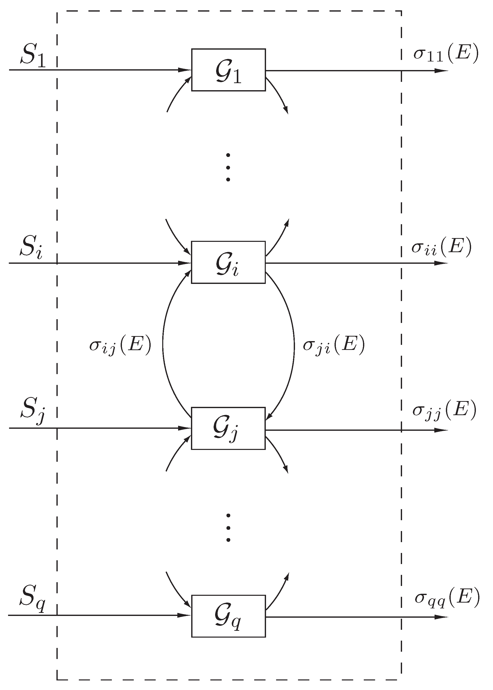
In this section, we extend the thermodynamic model proposed in [30] to include probabilistic variations in the instantaneous rate of energy dissipation as well as probabilistic variations in the energy transfer between the subsystems. Even though the treatment in this and the next two sections closely parallels that of [30] for deterministic thermodynamics, the thermodynamic models and proofs of our results are rendered more difficult due to the inclusion of stochastic disturbances. To formulate our state space stochastic thermodynamic model, we consider the large-scale stochastic dynamical system $\mathcal{G}$ shown in Figure 1 involving energy exchange between q interconnected subsystems and use the notation developed in [30].

Figure 1. Large-scale dynamical system $\mathcal{G}$ with $D\left(E\right)=0$ and $J\left(E\right)=0$.

Specifically, $E_i:[0,\infty )\to {\overline{\mathbb{R}}}_{+}$ denotes the energy (and hence a nonnegative quantity) of the i-th subsystem, $S_i:[0,\infty )\to \mathbb{R}$ denotes the external power (heat flux) supplied to (or extracted from) the i-th subsystem, ${\sigma }_{ij}:{\overline{\mathbb{R}}}_{+}^q\to {\overline{\mathbb{R}}}_{+}$, $i\ne j,i,j=1,\dots ,q$, denotes the instantaneous rate of energy (heat) flow from the j-th subsystem to the i-th subsystem, $J_{(i,k)}:{\overline{\mathbb{R}}}_{+}^q\to {\overline{\mathbb{R}}}_{+}$, $i=1,\dots ,q$, $k=1,\dots ,d_1$, denotes the instantaneous rate of energy (heat) received or delivered to the i-th subsystem from all other subsystems due to the stochastic disturbance $w_{1k}(·)$, ${\sigma }_{ii}:{\overline{\mathbb{R}}}_{+}^q\to {\overline{\mathbb{R}}}_{+},i=1,\dots ,q$, denotes the instantaneous rate of energy (heat) dissipation from the i-th subsystem to the environment, and $D_{(i,l)}:{\overline{\mathbb{R}}}_{+}^q\to {\overline{\mathbb{R}}}_{+},i=1,\dots ,q,l=1,\dots ,d_2$, denotes the instantaneous rate of energy (heat) dissipation from the i-th subsystem to the environment due to the stochastic disturbance $w_{2l}(·)$. Here we assume that ${\sigma }_{ij}:{\overline{\mathbb{R}}}_{+}^q\to {\overline{\mathbb{R}}}_{+},i,j=1,\dots ,q$, $J_{(i,k)}:{\overline{\mathbb{R}}}_{+}^q\to {\overline{\mathbb{R}}}_{+}$, $i=1,\dots ,q$, $k=1,\dots ,d_1$, and $D_{(i,l)}:{\overline{\mathbb{R}}}_{+}^q\to {\overline{\mathbb{R}}}_{+},i=1,\dots ,q,l=1,\dots ,d_2$, are locally Lipschitz continuous on ${\overline{\mathbb{R}}}_{+}^q$ and satisfy a linear growth condition, and $S_i:[0,\infty )\to \mathbb{R},i=1,\dots ,q$, are bounded piecewise continuous functions of time.

An energy balance for the i-th subsystem yields

$$\begin{array}{ccc}\hfill E_i\left(T\right)& =& E_i\left(t_0\right)+\sum _{j=1,j\ne i}^q{\int }_{t_0}^T[{\sigma }_{ij}\left(E\left(t\right)\right)-{\sigma }_{ji}\left(E\left(t\right)\right)]\mathrm{d}t\hfill \\ & & +{\int }_{t_0}^T{\mathrm{row}}_i\left(J\left(E\left(t\right)\right)\right)\mathrm{d}{w}_1\left(t\right)-{\int }_{t_0}^T{\sigma }_{ii}\left(E\left(t\right)\right)\mathrm{d}t\hfill \\ & & -{\int }_{t_0}^T{\mathrm{row}}_i\left(D\left(E\left(t\right)\right)\right)\mathrm{d}{w}_2\left(t\right)+{\int }_{t_0}^T{S}_i\left(t\right)\mathrm{d}t,T\ge t_0,\hfill \end{array}$$

(65)

or, equivalently, in vector form,

$$\begin{array}{ccc}\hfill E\left(T\right)& =& E\left(t_0\right)+{\int }_{t_0}^{T}f\left(E\left(t\right)\right)\mathrm{d}t+{\int }_{t_0}^{T}J\left(E\left(t\right)\right)\mathrm{d}{w}_1\left(t\right)-{\int }_{t_0}^{T}d\left(E\left(t\right)\right)\mathrm{d}t\hfill \\ & & -{\int }_{t_0}^{T}D\left(E\left(t\right)\right)\mathrm{d}{w}_2\left(t\right)+{\int }_{t_0}^{T}S\left(t\right)\mathrm{d}t,T\ge t_0,\hfill \end{array}$$

(66)

where $E\left(t\right)\triangleq {[E_1\left(t\right),\dots ,E_q\left(t\right)]}^{\mathrm{T}}$, $w_1(·)$ and $w_2(·)$ are, respectively, a $d_1$-dimensional and $d_2$-dimensional independent standard Wiener process (i.e., Brownian motion) defined on a complete filtered probability space $(\mathsf{\Omega },\mathcal{F},{\left\{{\mathcal{F}}_t\right\}}_{t\ge t_0},\mathbb{P})$, $E\left(t_0\right)$ is independent of $(w_1\left(t\right)-w_1\left(t_0\right)),t\ge t_0$, and $(w_2\left(t\right)-w_2\left(t_0\right)),t\ge t_0$,

$$\begin{array}{ccc}\hfill d\left(E\right(t\left)\right)& \triangleq & {[{\sigma }_{11}\left(E\left(t\right)\right),\dots ,{\sigma }_{qq}\left(E\left(t\right)\right)]}^{\mathrm{T}},\hfill \\ \hfill S\left(t\right)& \triangleq & {[S_1\left(t\right),\dots ,S_q\left(t\right)]}^{\mathrm{T}},\hfill \\ \hfill f\left(E\right)& =& {[f_1\left(E\right),\dots ,f_q\left(E\right)]}^{\mathrm{T}}:{\overline{\mathbb{R}}}_{+}^q\to {\mathbb{R}}^q,\hfill \\ \hfill J\left(E\right)& =& {[{\mathrm{row}}_1\left(J\left(E\right)\right),\dots ,{\mathrm{row}}_q\left(J\left(E\right)\right)]}^{\mathrm{T}}:{\overline{\mathbb{R}}}_{+}^q\to {\mathbb{R}}^q\times {\mathbb{R}}^{d_1},\hfill \\ \hfill D\left(E\right)& =& {[{\mathrm{row}}_1\left(D\left(E\right)\right),\dots ,{\mathrm{row}}_q\left(D\left(E\right)\right)]}^{\mathrm{T}}:{\overline{\mathbb{R}}}_{+}^q\to {\mathbb{R}}^q\times {\mathbb{R}}^{d_2}.\hfill \end{array}$$

Here, the stochastic disturbance $J\left(E\right)\mathrm{d}{w}_1$ in (66) captures probabilistic variations in the energy transfer rates between compartments and the stochastic disturbance $D\left(E\right)\mathrm{d}{w}_2$ captures probabilistic variations in the instantaneous rate of energy dissipation.

Equivalently, (65) can be rewritten as

$$\begin{array}{ccc}\hfill \mathrm{d}{E}_i\left(t\right)& =& \sum _{j=1,j\ne i}^q[{\sigma }_{ij}\left(E\left(t\right)\right)-{\sigma }_{ji}\left(E\left(t\right)\right)]\mathrm{d}t+{\mathrm{row}}_i\left(J\left(E\left(t\right)\right)\right)\mathrm{d}{w}_1\left(t\right)-{\sigma }_{ii}\left(E\left(t\right)\right)\mathrm{d}t\hfill \\ & & -{\mathrm{row}}_i\left(D\left(E\left(t\right)\right)\right)\mathrm{d}{w}_2\left(t\right)+S_i\left(t\right)\mathrm{d}t,E_i\left(t_0\right)\stackrel{\mathrm{a}.\mathrm{s}.}{=}{E}_{i0},t\ge t_0,\hfill \end{array}$$

(67)

or, in vector form,

$$\mathrm{d}E\left(t\right)=f\left(E\left(t\right)\right)\mathrm{d}t+J\left(E\left(t\right)\right)\mathrm{d}{w}_1\left(t\right)-d\left(E\left(t\right)\right)\mathrm{d}t-D\left(E\left(t\right)\right)\mathrm{d}{w}_2\left(t\right)+S\left(t\right)\mathrm{d}t,E\left(t_0\right)\stackrel{\mathrm{a}.\mathrm{s}.}{=}{E}_0,t\ge t_0,$$

(68)

where $E_0\triangleq {[E_{10},\dots ,E_{q0}]}^{\mathrm{T}}$, yielding a differential energy balance equation that characterizes energy flow between subsystems of the large-scale stochastic dynamical system $\mathcal{G}$. Here we assume that $S(·)$ satisfies sufficient regularity conditions such that (68) has a unique solution forward in time. Specifically, we assume that the external power (heat flux) $S(·)$ supplied to the large-scale stochastic dynamical system $\mathcal{G}$ consists of measurable functions $S(·)$ adapted to the filtration ${\left\{{\mathcal{F}}_t\right\}}_{t\ge t_0}$ such that $S\left(t\right)\in {\mathcal{H}}_q$, $t\ge t_0$, for all $t\ge s$, $w\left(t\right)-w\left(s\right)$ is independent of $S\left(\tau \right)$, $w\left(\tau \right)$, $\tau \le s$, and $E\left(t_0\right)$, where $w\left(t\right)\triangleq {[w_1^{\mathrm{T}}\left(t\right),w_2^{\mathrm{T}}\left(t\right)]}^{\mathrm{T}}$, and hence, $S(·)$ is non-anticipative. Furthermore, we assume that $S(·)$ takes values in a compact metrizable set. In this case, it follows from Theorem 2.2.4 of [53] that there exists a path-wise unique solution to (68) in $(\mathsf{\Omega },{\left\{{\mathcal{F}}_t\right\}}_{t\ge t_0},{\mathbb{P}}^{E_0})$.

Equation (66) or, equivalently, (68) is a statement of the first law for stochastic thermodynamics as applied to isochoric transformations (i.e., constant subsystem volume transformations) for each of the subsystems ${\mathcal{G}}_i,i=1,\dots ,q$. To see this, let the total energy in the large-scale stochastic dynamical system $\mathcal{G}$ be given by $U\triangleq {\mathbf{e}}^{\mathrm{T}}E$, where ${\mathbf{e}}^{\mathrm{T}}\triangleq [1,\dots ,1]$ and $E\in {\overline{\mathbb{R}}}_{+}^q$, and let the net energy received by the large-scale dynamical system $\mathcal{G}$ over the time interval $[t_1,t_2]$ be given by

$$\begin{array}{c}\hfill Q\triangleq {\int }_{t_1}^{t_2}{\mathbf{e}}^{\mathrm{T}}[S\left(t\right)-d\left(E\left(t\right)\right)]\mathrm{d}t-{\int }_{t_1}^{t_2}{\mathbf{e}}^{\mathrm{T}}D\left(E\left(t\right)\right)\mathrm{d}{w}_2\left(t\right),\end{array}$$

(69)

where $E\left(t\right),t\ge t_0$, is the solution to (68). Then, premultiplying (66) by ${\mathbf{e}}^{\mathrm{T}}$ and using the fact that ${\mathbf{e}}^{\mathrm{T}}f\left(E\right)\equiv 0$ and ${\mathbf{e}}^{\mathrm{T}}J\left(E\right)\equiv 0$, it follows that

$$\begin{array}{c}\hfill \Delta U=Q,\end{array}$$

(70)

where $\Delta U\triangleq U\left(t_2\right)-U\left(t_1\right)$ denotes the variation in the total energy of the large-scale stochastic dynamical system $\mathcal{G}$ over the time interval $[t_1,t_2]$.

For our large-scale stochastic dynamical system model $\mathcal{G}$, we assume that ${\sigma }_{ij}\left(E\right)=0,E\in {\overline{\mathbb{R}}}_{+}^q$, ${\sigma }_{jj}\left(E\right)=0,E\in {\overline{\mathbb{R}}}_{+}^q$, $J_{(j,k)}\left(E\right)=0,E\in {\overline{\mathbb{R}}}_{+}^q$, $k=1,\dots ,d_1$, and $D_{(j,l)}\left(E\right)=0,E\in {\overline{\mathbb{R}}}_{+}^q$, $l=1,\dots ,d_2$, whenever $E_j=0,j=1,\dots ,q$. In this case, $f\left(E\right)-d\left(E\right),E\in {\overline{\mathbb{R}}}_{+}^q$, is essentially nonnegative. The above constraint implies that if the energy of the j-th subsystem of $\mathcal{G}$ is zero, then this subsystem cannot supply any energy to its surroundings nor dissipate energy to the environment. Moreover, we assume that $S_i\left(t\right)\ge 0$ whenever $E_i\left(t\right)=0$, $t\ge t_0$, $i=1,\dots ,q$, which implies that when the energy of the i-th subsystem is zero, then no energy can be extracted from this subsystem.

The following proposition is needed for the main results of this paper.

Proposition 4.

Consider the large-scale stochastic dynamical system $\mathcal{G}$ with differential energy balance equation given by (68). Suppose ${\sigma }_{ij}\left(E\right)=0$, $E\in {\overline{\mathbb{R}}}_{+}^q$, $J_{(j,k)}\left(E\right)=0,E\in {\overline{\mathbb{R}}}_{+}^q$, $k=1,\dots ,d_1$, and $D_{(j,l)}\left(E\right)=0,E\in {\overline{\mathbb{R}}}_{+}^q$, $l=1,\dots ,d_2$, whenever $E_j=0$, $j=1,\dots ,q$, and $S_i\left(t\right)\ge 0$ whenever $E_i\left(t\right)=0$, $t\ge t_0$, $i=1,\dots ,q$. Then the solution $E\left(t\right)$, $t\ge t_0$, to (68) is nonnegative for all nonnegative initial conditions $E_0\in {\overline{\mathbb{R}}}_{+}^q$.

Proof. 

First note that $f\left(E\right)-d\left(E\right),E\in {\overline{\mathbb{R}}}_{+}^q$, is essentially nonnegative, $J_{(j,k)}\left(E\right)=0,E\in {\overline{\mathbb{R}}}_{+}^q$, $k=1,\dots ,d_1$, and $D_{(j,l)}\left(E\right)=0,E\in {\overline{\mathbb{R}}}_{+}^q$, $l=1,\dots ,d_2$, whenever $E_j=0$, $j=1,\dots ,q$. Next, since $S_i\left(t\right)\ge 0$ whenever $E_i\left(t\right)=0$, $t\ge t_0$, $i=1,\dots ,q$, it follows that $\mathrm{d}{E}_i\left(t\right)\ge 0$ for all $t\ge t_0$ and $i=1,\dots ,q$ whenever $E_i\left(t\right)=0$ and $E_j\left(t\right)\ge 0$ for all $j\ne i$ and $t\ge t_0$. This implies that for all nonnegative initial conditions $E_0\in {\overline{\mathbb{R}}}_{+}^q$, every sample trajectory of $\mathcal{G}$ is directed towards the interior of the nonnegative orthant ${\overline{\mathbb{R}}}_{+}^q$ whenever $E_i\left(t\right)=0,i=1,\dots ,q$, and hence, remains nonnegative almost surely for all $t\ge t_0$. ☐

Next, premultiplying (66) by ${\mathbf{e}}^{\mathrm{T}}$, using Proposition 4, and using the fact that ${\mathbf{e}}^{\mathrm{T}}f\left(E\right)\equiv 0$ and ${\mathbf{e}}^{\mathrm{T}}J\left(E\right)\equiv 0$, it follows that

$$\begin{array}{ccc}\hfill {\mathbf{e}}^{\mathrm{T}}E\left(T\right)& =& {\mathbf{e}}^{\mathrm{T}}E\left(t_0\right)+{\int }_{t_0}^T{\mathbf{e}}^{\mathrm{T}}S\left(t\right)\mathrm{d}t-{\int }_{t_0}^T{\mathbf{e}}^{\mathrm{T}}d\left(E\left(t\right)\right)\mathrm{d}t-{\int }_{t_0}^T{\mathbf{e}}^{\mathrm{T}}D\left(E\left(t\right)\right)\mathrm{d}{w}_2\left(t\right),T\ge t_0.\hfill \end{array}$$

(71)

Now, for the large-scale stochastic dynamical system $\mathcal{G}$, define the input $u\left(t\right)\triangleq S\left(t\right)$ and the output $y\left(t\right)\triangleq d\left(E\right(t\left)\right)$. Hence, it follows from (71) that for any two ${\mathcal{F}}_t$-stopping times ${\tau }_1$ and ${\tau }_2$ such that ${\tau }_1\ge {\tau }_2$ almost surely,

$$\begin{array}{ccc}\hfill \mathbb{E}\left[{\mathbf{e}}^{\mathrm{T}}E\left({\tau }_2\right)|{\mathcal{F}}_{{\tau }_1}\right]& =& {\mathbf{e}}^{\mathrm{T}}E\left({\tau }_1\right)+\mathbb{E}\left[{\int }_{{\tau }_1}^{{\tau }_2}{\mathbf{e}}^{\mathrm{T}}S\left(t\right)\mathrm{d}t|{\mathcal{F}}_{{\tau }_1}\right]-\mathbb{E}\left[{\int }_{{\tau }_1}^{{\tau }_2}{\mathbf{e}}^{\mathrm{T}}d\left(E\left(t\right)\right)\mathrm{d}t|{\mathcal{F}}_{{\tau }_1}\right]\hfill \\ & & -\mathbb{E}\left[{\int }_{{\tau }_1}^{{\tau }_2}{\mathbf{e}}^{\mathrm{T}}D\left(E\left(t\right)\right)\mathrm{d}{w}_2\left(t\right)|{\mathcal{F}}_{{\tau }_1}\right]\hfill \\ & =& {\mathbf{e}}^{\mathrm{T}}E\left({\tau }_1\right)+\mathbb{E}\left[{\int }_{{\tau }_1}^{{\tau }_2}\left[{\mathbf{e}}^{\mathrm{T}}S\left(t\right)-{\mathbf{e}}^{\mathrm{T}}d\left(E\left(t\right)\right)\right]\mathrm{d}t|{\mathcal{F}}_{{\tau }_1}\right].\hfill \end{array}$$

(72)

Thus, the large-scale stochastic dynamical system $\mathcal{G}$ is stochastically lossless [54] with respect to the energy supply rate $r(u,y)\triangleq {\mathbf{e}}^{\mathrm{T}}u-{\mathbf{e}}^{\mathrm{T}}y$ and with the energy storage function $U\left(E\right)\triangleq {\mathbf{e}}^{\mathrm{T}}E,E\in {\overline{\mathbb{R}}}_{+}^q$. In other words, the difference between the supplied system energy and the stored system energy is a martingale with respect to the differential energy balance system filtration.

The following lemma is required for our next result.

Lemma 2.

Consider the large-scale stochastic dynamical system $\mathcal{G}$ with differential energy balance Equation (68). Then, for every equilibrium state $E_{\mathrm{e}}\in {\mathcal{H}}_q^{+}$ and every $\epsilon >0$ and $\tau \stackrel{\mathrm{a}.\mathrm{s}.}{>}0$, there exist $S_{\mathrm{e}}\in {\mathcal{H}}_q$, $\alpha >0$, and $\tau \stackrel{\mathrm{a}.\mathrm{s}.}{>}\widehat{\tau }\stackrel{\mathrm{a}.\mathrm{s}.}{>}0$ such that, for every $\widehat{E}\in {\mathcal{H}}_q^{+}$ with $\parallel \widehat{E}-E_{\mathrm{e}}\parallel \stackrel{\mathrm{a}.\mathrm{s}.}{\le }\alpha \tau$, there exists $S:{\overline{\mathbb{R}}}_{+}\to {\mathcal{H}}_q$ such that $\parallel S\left(t\right)-S_{\mathrm{e}}\parallel \stackrel{\mathrm{a}.\mathrm{s}.}{\le }\epsilon$, $t\in [0,\widehat{\tau }]$, and $E\left(t\right)=E_{\mathrm{e}}+\frac{(\widehat{E}-E_{\mathrm{e}})}{\widehat{\tau }}t$, $t\in [0,\widehat{\tau }]$.

Proof. 

Note that with $S_{\mathrm{e}}\triangleq d\left(E_{\mathrm{e}}\right)-f\left(E_{\mathrm{e}}\right)$, the state $E_{\mathrm{e}}\in {\overline{\mathbb{R}}}_{+}^q$ is an equilibrium state of (68). Let $\theta >0$ and $\tau \stackrel{\mathrm{a}.\mathrm{s}.}{>}0$, and define

$$\begin{array}{ccc}\hfill M(\theta ,\tau )& \triangleq & \underset{E\in {\mathcal{H}}_q^{{\overline{\mathcal{B}}}_1\left(0\right)},t\in [0,\tau ]}{sup}\parallel f(E_{\mathrm{e}}+\theta tE)-d(E_{\mathrm{e}}+\theta tE)+S_{\mathrm{e}}\parallel ,\hfill \end{array}$$

(73)

$$\begin{array}{ccc}\hfill M_J(\theta ,\tau )& \triangleq & \underset{E\in {\mathcal{H}}_q^{{\overline{\mathcal{B}}}_1\left(0\right)},t\in [0,\tau ]}{sup}∥J\left(E_{\mathrm{e}}+\frac{(\widehat{E}-E_{\mathrm{e}})}{\parallel \widehat{E}-E_{\mathrm{e}}\parallel }\alpha t\right)∥,\hfill \end{array}$$

(74)

$$\begin{array}{ccc}\hfill M_D(\theta ,\tau )& \triangleq & \underset{E\in {\mathcal{H}}_q^{{\overline{\mathcal{B}}}_1\left(0\right)},t\in [0,\tau ]}{sup}∥D\left(E_{\mathrm{e}}+\frac{(\widehat{E}-E_{\mathrm{e}})}{\parallel \widehat{E}-E_{\mathrm{e}}\parallel }\alpha t\right)∥.\hfill \end{array}$$

(75)

Note that for every $\tau \stackrel{\mathrm{a}.\mathrm{s}.}{>}0$, ${lim}_{\theta \to 0^{+}}M(\theta ,\tau )\stackrel{\mathrm{a}.\mathrm{s}.}{=}0$, ${lim}_{\theta \to 0^{+}}{M}_J(\theta ,\tau )\stackrel{\mathrm{a}.\mathrm{s}.}{=}0$, and ${lim}_{\theta \to 0^{+}}{M}_D(\theta ,\tau )\stackrel{\mathrm{a}.\mathrm{s}.}{=}0$, and for every $\theta >0$, ${lim}_{\tau \stackrel{\mathrm{a}.\mathrm{s}.}{\to }{0}^{+}}M(\theta ,\tau )\stackrel{\mathrm{a}.\mathrm{s}.}{=}0$, ${lim}_{\tau \stackrel{\mathrm{a}.\mathrm{s}.}{\to }{0}^{+}}{M}_J(\theta ,\tau )\stackrel{\mathrm{a}.\mathrm{s}.}{=}0$, and ${lim}_{\tau \stackrel{\mathrm{a}.\mathrm{s}.}{\to }{0}^{+}}{M}_D(\theta ,\tau )\stackrel{\mathrm{a}.\mathrm{s}.}{=}0$. Moreover, it follows from Lévy’s modulus of continuity theorem [55] that for sufficiently small $\mathrm{d}t>0$, $\parallel \mathrm{d}{w}_1\left(t\right)\parallel \stackrel{\mathrm{a}.\mathrm{s}.}{\le }{M}_W\left(\mathrm{d}t\right)\mathrm{d}t$ and $\parallel \mathrm{d}{w}_2\left(t\right)\parallel \stackrel{\mathrm{a}.\mathrm{s}.}{\le }{M}_W\left(\mathrm{d}t\right)\mathrm{d}t$, where $M_W\left(\mathrm{d}t\right)\triangleq \sqrt{2\mathrm{d}t{log}_e\left(\frac{1}{\mathrm{d}t}\right)}$.

Next, let $\epsilon >0$ and $\tau \stackrel{\mathrm{a}.\mathrm{s}.}{>}0$ be given and, for sufficiently small $\mathrm{d}t>0$, let $\alpha >0$ be such that

$$M(\alpha ,\tau )+\alpha +M_J(\alpha ,\tau )M_W\left(\mathrm{d}t\right)+M_D(\alpha ,\tau )M_W\left(\mathrm{d}t\right)\stackrel{\mathrm{a}.\mathrm{s}.}{\le }\epsilon .$$

(The existence of such an $\alpha$ is guaranteed since $M(\alpha ,\tau )\stackrel{\mathrm{a}.\mathrm{s}.}{\to }0$, $M_J(\alpha ,\tau )\stackrel{\mathrm{a}.\mathrm{s}.}{\to }0$, and $M_D(\alpha ,\tau )\stackrel{\mathrm{a}.\mathrm{s}.}{\to }0$ as $\alpha \to 0^{+}$.) Now, let $\widehat{E}\in {\mathcal{H}}_q^{+}$ be such that $\parallel \widehat{E}-E_{\mathrm{e}}\parallel \stackrel{\mathrm{a}.\mathrm{s}.}{\le }\alpha \tau$. With $\widehat{\tau }\triangleq \frac{\parallel \widehat{E}-E_{\mathrm{e}}\parallel }{\alpha }\stackrel{\mathrm{a}.\mathrm{s}.}{\le }\tau$ and

$$\begin{array}{ccc}\hfill S\left(t\right)\mathrm{d}t& =& \left[-f\left(E\left(t\right)\right)+d\left(E\left(t\right)\right)+\alpha \frac{(\widehat{E}-E_{\mathrm{e}})}{\parallel \widehat{E}-E_{\mathrm{e}}\parallel }\right]\mathrm{d}t\hfill \\ & & -J\left(E\left(t\right)\right)\mathrm{d}{w}_1\left(t\right)+D\left(E\left(t\right)\right)\mathrm{d}{w}_2\left(t\right),t\in [0,\widehat{\tau }],\hfill \end{array}$$

(76)

it follows that

$$\begin{array}{c}\hfill E\left(t\right)=E_{\mathrm{e}}+\frac{(\widehat{E}-E_{\mathrm{e}})}{\parallel \widehat{E}-E_{\mathrm{e}}\parallel }\alpha t,t\in [0,\widehat{\tau }],\end{array}$$

(77)

is a solution to (68).

The result is now immediate by noting that $E\left(\widehat{\tau }\right)\stackrel{\mathrm{a}.\mathrm{s}.}{=}\widehat{E}$ and

$$\begin{array}{ccc}\hfill \parallel S\left(t\right)-S_{\mathrm{e}}\parallel \mathrm{d}t& \stackrel{\mathrm{a}.\mathrm{s}.}{\le }& ∥f\left(E_{\mathrm{e}}+\frac{(\widehat{E}-E_{\mathrm{e}})}{\parallel \widehat{E}-E_{\mathrm{e}}\parallel }\alpha t\right)-d\left(E_{\mathrm{e}}+\frac{(\widehat{E}-E_{\mathrm{e}})}{\parallel \widehat{E}-E_{\mathrm{e}}\parallel }\alpha t\right)+S_{\mathrm{e}}∥\mathrm{d}t\hfill \\ & & +\alpha \mathrm{d}t+∥J\left(E_{\mathrm{e}}+\frac{(\widehat{E}-E_{\mathrm{e}})}{\parallel \widehat{E}-E_{\mathrm{e}}\parallel }\alpha t\right)∥\left|\mathrm{d}{w}_1\left(t\right)\right|\hfill \\ & & +∥D\left(E_{\mathrm{e}}+\frac{(\widehat{E}-E_{\mathrm{e}})}{\parallel \widehat{E}-E_{\mathrm{e}}\parallel }\alpha t\right)∥\left|\mathrm{d}{w}_2\left(t\right)\right|\hfill \\ & \stackrel{\mathrm{a}.\mathrm{s}.}{\le }& [M(\alpha ,\tau )+\alpha +M_J(\alpha ,\tau )M_W\left(\mathrm{d}t\right)+M_D(\alpha ,\tau )M_W\left(\mathrm{d}t\right)]\mathrm{d}t,t\in [0,\widehat{\tau }],\hfill \end{array}$$

(78)

and hence,

$$\begin{array}{cc}\hfill \parallel S\left(t\right)-S_{\mathrm{e}}\parallel & \stackrel{\mathrm{a}.\mathrm{s}.}{\le }M(\alpha ,\tau )+\alpha +M_J(\alpha ,\tau )M_W\left(\mathrm{d}t\right)+M_D(\alpha ,\tau )M_W\left(\mathrm{d}t\right)\stackrel{\mathrm{a}.\mathrm{s}.}{\le }\epsilon ,\hfill \end{array}$$

which proves the result. ☐

It follows from Lemma 2 that the large-scale stochastic dynamical system $\mathcal{G}$ with the differential energy balance Equation (68) is stochastically reachable from and stochastically controllable to the origin in ${\overline{\mathbb{R}}}_{+}^q$. Recall from [54] that the large-scale stochastic dynamical system $\mathcal{G}$ with the differential energy balance Equation (68) is stochastically reachable from the origin in ${\overline{\mathbb{R}}}_{+}^q$ if, for all $E_0\in {\overline{\mathbb{R}}}_{+}^q$ and $\epsilon >0$, there exist a finite random variable ${\tau }_{{\mathcal{B}}_{\epsilon }\left(E_0\right)}\stackrel{\mathrm{a}.\mathrm{s}.}{\ge }{t}_0$, called the first hitting time, defined by

$${\tau }_{{\mathcal{B}}_{\epsilon }\left(E_0\right)}\left(\omega \right)\triangleq inf\{t\ge t_0:E(t,\omega )\in {\mathcal{B}}_{\epsilon }\left(E_0\right)\},$$

and a ${\mathcal{F}}_t$-adapted square integrable input $S(·)$ defined on $[t_0,{\tau }_{{\mathcal{B}}_{\epsilon }\left(E_0\right)}]$ such that the state $E\left(t\right)$, $t\ge t_0$, can be driven from $E\left(t_0\right)\stackrel{\mathrm{a}.\mathrm{s}.}{=}0$ to $E\left({\tau }_{{\mathcal{B}}_{\epsilon }\left(E_0\right)}\right)$ and $\mathbb{E}\left[{\tau }_{E_0}\right]<\infty$, where ${\tau }_{E_0}\triangleq {sup}_{\epsilon >0}{\tau }_{{\mathcal{B}}_{\epsilon }\left(E_0\right)}$ and the supremum is taken pointwise. Alternatively, $\mathcal{G}$ is stochastically controllable to the origin in ${\overline{\mathbb{R}}}_{+}^q$ if, for all $E\left(t_0\right)\stackrel{\mathrm{a}.\mathrm{s}.}{=}{E}_0$, $E_0\in {\overline{\mathbb{R}}}_{+}^q$, there exists a finite random variable ${\tilde{\tau }}_{{\mathcal{B}}_{\epsilon }\left(E_0\right)}\stackrel{\mathrm{a}.\mathrm{s}.}{\ge }{t}_0$ defined by

$${\tilde{\tau }}_{{\mathcal{B}}_{\epsilon }\left(E_0\right)}\left(\omega \right)\triangleq inf\{t\ge t_0:E(t,\omega )\in {\mathcal{B}}_{\epsilon }\left(0\right)\},$$

and a ${\mathcal{F}}_t$-adapted square integrable input $S(·)$ defined on $[t_0,{\tilde{\tau }}_{{\mathcal{B}}_{\epsilon }\left(E_0\right)}]$ such that the state $E\left(t\right),t\ge t_0$, can be driven from $E\left(t_0\right)\stackrel{\mathrm{a}.\mathrm{s}.}{=}{E}_0$ to $E\left({\tilde{\tau }}_{{\mathcal{B}}_{\epsilon }\left(E_0\right)}\right)\in {\mathcal{B}}_{\epsilon }\left(0\right)$ and ${\tilde{\tau }}_{E_0}\triangleq {sup}_{\epsilon >0}{\tilde{\tau }}_{{\mathcal{B}}_{\epsilon }\left(E_0\right)}$ with a pointwise supremum.

We let ${\mathcal{U}}_{\mathrm{r}}$ denote the set of measurable bounded ${\mathcal{H}}_q^{+}$-valued stochastic processes on the semi-infinite interval $[t_0,\infty )$ consisting of power inputs (heat fluxes) to the large-scale stochastic dynamical system $\mathcal{G}$ such that for every ${\tau }_{E_0}\stackrel{\mathrm{a}.\mathrm{s}.}{\ge }{t}_0$ the system energy state can be driven from $E\left(t_0\right)\stackrel{\mathrm{a}.\mathrm{s}.}{=}0$ to $E\left({\tau }_{E_0}\right)$ by $S(·)\in {\mathcal{U}}_{\mathrm{r}}$. Furthermore, we let ${\mathcal{U}}_{\mathrm{c}}$ denote the set of measurable bounded ${\mathcal{H}}_q^{+}$-valued stochastic processes on the semi-infinite interval $[t_0,\infty )$ consisting of power inputs (heat fluxes) to the large-scale stochastic dynamical system $\mathcal{G}$ such that the system energy state can be driven from $E\left(t_0\right)\stackrel{\mathrm{a}.\mathrm{s}.}{=}{E}_0$, $E_0\in {\overline{\mathbb{R}}}_{+}^q$ to $E\left({\tilde{\tau }}_{E_0}\right)$ by $S(·)\in {\mathcal{U}}_{\mathrm{c}}$. Finally, let $\mathcal{U}$ be an input space that is a subset of measurable bounded ${\mathcal{H}}_q^{+}$-valued stochastic processes on $\mathbb{R}$. The spaces ${\mathcal{U}}_{\mathrm{r}}$, ${\mathcal{U}}_{\mathrm{c}}$, and $\mathcal{U}$ are assumed to be closed under the shift operator, that is, if $S(·)\in \mathcal{U}$ (respectively, ${\mathcal{U}}_{\mathrm{c}}$ or ${\mathcal{U}}_{\mathrm{r}}$), then the function $S_T$ defined by $S_T\left(t\right)\triangleq S(t+T)$ is contained in $\mathcal{U}$ (respectively, ${\mathcal{U}}_{\mathrm{c}}$ or ${\mathcal{U}}_{\mathrm{r}}$) for all $T\ge 0$.

The next result establishes the uniqueness of the internal energy function $U\left(E\right),E\in {\overline{\mathbb{R}}}_{+}^q$, for our large-scale stochastic dynamical system $\mathcal{G}$. For this result define the available energy of the large-scale stochastic dynamical system $\mathcal{G}$ by

$$\begin{array}{ccc}\hfill U_{\mathrm{a}}\left(E_0\right)& \triangleq & -\underset{u(·)\in \mathcal{U},\tau \stackrel{\mathrm{a}.\mathrm{s}.}{\ge }{t}_0}{inf}\mathbb{E}\left[\mathbb{E}\left[{\int }_{t_0}^{\tau }[{\mathbf{e}}^{\mathrm{T}}u\left(t\right)-{\mathbf{e}}^{\mathrm{T}}y\left(t\right)]\mathrm{d}t|E\left(t_0\right)\stackrel{\mathrm{a}.\mathrm{s}.}{=}{E}_0\right]\right],E_0\in {\overline{\mathbb{R}}}_{+}^q,\hfill \end{array}$$

(79)

where $E\left(t\right)$, $t\ge t_0$, is the solution to (68) with $E\left(t\right)\stackrel{\mathrm{a}.\mathrm{s}.}{=}{E}_0$ and admissible inputs $S(·)\in \mathcal{U}$. The infimum in (79) is taken over all ${\mathcal{F}}_t$-measurable inputs $S(·)$, all finite ${\mathcal{F}}_t$-stopping times $\tau \stackrel{\mathrm{a}.\mathrm{s}.}{\ge }0$, and all system sample paths with initial value $E\left(t_0\right)\stackrel{\mathrm{a}.\mathrm{s}.}{=}{E}_0$ and terminal value left free. Furthermore, define the required energy supply of the large-scale stochastic dynamical system $\mathcal{G}$ by

$$\begin{array}{ccc}\hfill U_{\mathrm{r}}\left(E_0\right)& \triangleq & \underset{u(·)\in {\mathcal{U}}_{\mathrm{r}},{\tau }_{E_0}\stackrel{\mathrm{a}.\mathrm{s}.}{\ge }0}{inf}\mathbb{E}\left[\mathbb{E}\left[{\int }_0^{{\tau }_{E_0}}[{\mathbf{e}}^{\mathrm{T}}u\left(t\right)-{\mathbf{e}}^{\mathrm{T}}y\left(t\right)]\mathrm{d}t|E\left(0\right)\stackrel{\mathrm{a}.\mathrm{s}.}{=}0\right]\right],E_0\in {\overline{\mathbb{R}}}_{+}^q.\hfill \end{array}$$

(80)

The infimum in (80) is taken over all system sample paths starting from $E\left(t_0\right)\stackrel{\mathrm{a}.\mathrm{s}.}{=}0$ and ending at $E\left({\tau }_{E_0}\right)\stackrel{\mathrm{a}.\mathrm{s}.}{=}{E}_0$ at time $t={\tau }_{E_0}$, and all times $t\ge t_0$.

Note that the available energy $U_{\mathrm{a}}\left(E\right)$ is the maximum amount of stored energy (net heat) that can be extracted from the large-scale stochastic dynamical system $\mathcal{G}$ at any finite stopping time $\tau$, and the required energy supply $U_{\mathrm{r}}\left(E\right)$ is the minimum amount of energy (net heat) that can be delivered to the large-scale stochastic dynamical system $\mathcal{G}$ such that, for all $\epsilon >0$, ${\mathbb{P}}^0\left({lim}_{t\to {\tau }_{E_0}}E\left(t\right)\in {\mathcal{B}}_{\epsilon }\left(E_0\right)\right)=1$.

Theorem 6.

Consider the large-scale stochastic dynamical system $\mathcal{G}$ with differential energy balance equation given by (68). Then $\mathcal{G}$ is stochastically lossless with respect to the energy supply rate $r(u,y)={\mathbf{e}}^{\mathrm{T}}u-{\mathbf{e}}^{\mathrm{T}}y$, where $u\left(t\right)\equiv S\left(t\right)$ and $y\left(t\right)\equiv d\left(E\right(t\left)\right)$, and with the unique energy storage function corresponding to the total energy of the system $\mathcal{G}$ given by

$$\begin{array}{ccc}\hfill U\left(E_0\right)& =& {\mathbf{e}}^{\mathrm{T}}{E}_0\hfill \\ & =& -\mathbb{E}\left[\mathbb{E}\left[{\int }_0^{{\tau }_0}[{\mathbf{e}}^{\mathrm{T}}u\left(t\right)-{\mathbf{e}}^{\mathrm{T}}y\left(t\right)]\mathrm{d}t|E\left(0\right)\stackrel{\mathrm{a}.\mathrm{s}.}{=}{E}_0\right]\right]\hfill \\ & =& \mathbb{E}\left[\mathbb{E}\left[{\int }_0^{{\tau }_{E_0}}[{\mathbf{e}}^{\mathrm{T}}u\left(t\right)-{\mathbf{e}}^{\mathrm{T}}y\left(t\right)]\mathrm{d}t|E\left(0\right)\stackrel{\mathrm{a}.\mathrm{s}.}{=}0\right]\right],E_0\in {\overline{\mathbb{R}}}_{+}^q,\hfill \end{array}$$

(81)

where $E\left(t\right)$, $t\ge t_0$, is the solution to (68) with admissible input $u(·)\in \mathcal{U}$, $E\left({\tau }_0\right)\stackrel{\mathrm{a}.\mathrm{s}.}{=}0$, and $E\left({\tau }_{E_0}\right)\stackrel{\mathrm{a}.\mathrm{s}.}{=}{E}_0\in {\overline{\mathbb{R}}}_{+}^q$. Furthermore,

$$\begin{array}{c}\hfill 0\le U_{\mathrm{a}}\left(E_0\right)=U\left(E_0\right)=U_{\mathrm{r}}\left(E_0\right)<\infty ,E_0\in {\overline{\mathbb{R}}}_{+}^q.\end{array}$$

(82)

Proof. 

Note that it follows from (71) that $\mathcal{G}$ is stochastically lossless with respect to the energy supply rate $r(u,y)={\mathbf{e}}^{\mathrm{T}}u-{\mathbf{e}}^{\mathrm{T}}y$ and with the energy storage function $U\left(E\right)={\mathbf{e}}^{\mathrm{T}}E,E\in {\overline{\mathbb{R}}}_{+}^q$. Since, by Lemma 2, $\mathcal{G}$ is reachable from and controllable to the origin in ${\overline{\mathbb{R}}}_{+}^q$, it follows from (71), with $E\left(t_0\right)\stackrel{\mathrm{a}.\mathrm{s}.}{=}{E}_0\in {\overline{\mathbb{R}}}_{+}^q$ and $E\left({\tau }_{+}\right)\stackrel{\mathrm{a}.\mathrm{s}.}{=}0$ for some ${\tau }_{+}\stackrel{\mathrm{a}.\mathrm{s}.}{\ge }{t}_0$ and $u(·)\in \mathcal{U}$, that

$$\begin{array}{ccc}\hfill {\mathbf{e}}^{\mathrm{T}}{E}_0& =& -\mathbb{E}\left[\mathbb{E}\left[{\int }_{t_0}^{{\tau }_{+}}[{\mathbf{e}}^{\mathrm{T}}u\left(t\right)-{\mathbf{e}}^{\mathrm{T}}y\left(t\right)]\mathrm{d}t|E\left(t_0\right)\stackrel{\mathrm{a}.\mathrm{s}.}{=}{E}_0\right]\right]\hfill \\ & \le & \underset{u(·)\in \mathcal{U},{\tau }_{+}\stackrel{\mathrm{a}.\mathrm{s}.}{\ge }{t}_0}{sup}-\mathbb{E}\left[\mathbb{E}\left[{\int }_{t_0}^{{\tau }_{+}}[{\mathbf{e}}^{\mathrm{T}}u\left(t\right)-{\mathbf{e}}^{\mathrm{T}}y\left(t\right)]\mathrm{d}t|E\left(t_0\right)\stackrel{\mathrm{a}.\mathrm{s}.}{=}{E}_0\right]\right]\hfill \\ & =& -\underset{u(·)\in \mathcal{U},{\tau }_{+}\stackrel{\mathrm{a}.\mathrm{s}.}{\ge }{t}_0}{inf}\mathbb{E}\left[\mathbb{E}\left[{\int }_{t_0}^{{\tau }_{+}}[{\mathbf{e}}^{\mathrm{T}}u\left(t\right)-{\mathbf{e}}^{\mathrm{T}}y\left(t\right)]\mathrm{d}t|E\left(t_0\right)\stackrel{\mathrm{a}.\mathrm{s}.}{=}{E}_0\right]\right]\hfill \\ & =& U_{\mathrm{a}}\left(E_0\right),E_0\in {\overline{\mathbb{R}}}_{+}^q.\hfill \end{array}$$

(83)

Alternatively, it follows from (71), with $E\left(0\right)\stackrel{\mathrm{a}.\mathrm{s}.}{=}0$ for some ${\tau }_{-}\stackrel{\mathrm{a}.\mathrm{s}.}{\ge }0$ and $u(·)\in {\mathcal{U}}_{\mathrm{r}}$, that

$$\begin{array}{ccc}\hfill {\mathbf{e}}^{\mathrm{T}}{E}_0& =& \mathbb{E}\left[\mathbb{E}\left[{\int }_0^{{\tau }_{-}}[{\mathbf{e}}^{\mathrm{T}}u\left(t\right)-{\mathbf{e}}^{\mathrm{T}}y\left(t\right)]\mathrm{d}t|E\left(0\right)\stackrel{\mathrm{a}.\mathrm{s}.}{=}0\right]\right]\hfill \\ & \ge & \underset{u(·)\in {\mathcal{U}}_{\mathrm{r}},{\tau }_{-}\stackrel{\mathrm{a}.\mathrm{s}.}{\ge }0}{inf}\mathbb{E}\left[\mathbb{E}\left[{\int }_0^{{\tau }_{-}}[{\mathbf{e}}^{\mathrm{T}}u\left(t\right)-{\mathbf{e}}^{\mathrm{T}}y\left(t\right)]\mathrm{d}t|E\left(0\right)\stackrel{\mathrm{a}.\mathrm{s}.}{=}0\right]\right]\hfill \\ & =& U_{\mathrm{r}}\left(E_0\right),E_0\in {\overline{\mathbb{R}}}_{+}^q.\hfill \end{array}$$

(84)

Thus, (83) and (84) imply that (81) is satisfied and

$$\begin{array}{c}\hfill U_{\mathrm{r}}\left(E_0\right)\le {\mathbf{e}}^{\mathrm{T}}{E}_0\le U_{\mathrm{a}}\left(E_0\right),E_0\in {\overline{\mathbb{R}}}_{+}^q.\end{array}$$

(85)

Conversely, it follows from (71) and the fact that $U\left(E\right)={\mathbf{e}}^{\mathrm{T}}E\ge 0,E\in {\overline{\mathbb{R}}}_{+}^q$, that, for all $\tau \stackrel{\mathrm{a}.\mathrm{s}.}{\ge }{t}_0$ and $u(·)\in \mathcal{U}$,

$$\begin{array}{c}\hfill {\mathbf{e}}^{\mathrm{T}}{E}_0\ge -\mathbb{E}\left[\mathbb{E}\left[{\int }_{t_0}^{\tau }[{\mathbf{e}}^{\mathrm{T}}u\left(t\right)-{\mathbf{e}}^{\mathrm{T}}y\left(t\right)]\mathrm{d}t|E\left(t_0\right)\stackrel{\mathrm{a}.\mathrm{s}.}{=}{E}_0\right]\right],E_0\in {\overline{\mathbb{R}}}_{+}^q,\end{array}$$

(86)

which implies that

$$\begin{array}{ccc}\hfill {\mathbf{e}}^{\mathrm{T}}E\left(t_0\right)& \ge & \underset{u(·)\in \mathcal{U},\tau \stackrel{\mathrm{a}.\mathrm{s}.}{\ge }{t}_0}{sup}-\mathbb{E}\left[\mathbb{E}\left[{\int }_{t_0}^{\tau }[{\mathbf{e}}^{\mathrm{T}}u\left(t\right)-{\mathbf{e}}^{\mathrm{T}}y\left(t\right)]\mathrm{d}t|E\left(t_0\right)\stackrel{\mathrm{a}.\mathrm{s}.}{=}{E}_0\right]\right]\hfill \\ & =& -\underset{u(·)\in \mathcal{U},\tau \stackrel{\mathrm{a}.\mathrm{s}.}{\ge }{t}_0}{inf}\mathbb{E}\left[\mathbb{E}\left[{\int }_{t_0}^{\tau }[{\mathbf{e}}^{\mathrm{T}}u\left(t\right)-{\mathbf{e}}^{\mathrm{T}}y\left(t\right)]\mathrm{d}t|E\left(t_0\right)\stackrel{\mathrm{a}.\mathrm{s}.}{=}{E}_0\right]\right]\hfill \\ & =& U_{\mathrm{a}}\left(E_0\right),E_0\in {\overline{\mathbb{R}}}_{+}^q.\hfill \end{array}$$

(87)

Furthermore, it follows from the definition of $U_{\mathrm{a}}(·)$ that $U_{\mathrm{a}}\left(E\right)\ge 0,E\in {\overline{\mathbb{R}}}_{+}^q$, since the infimum in (79) is taken over the set of values containing the zero value ($\tau \stackrel{\mathrm{a}.\mathrm{s}.}{=}{t}_0$).

Next, note that it follows from (71), with $E\left(0\right)\stackrel{\mathrm{a}.\mathrm{s}.}{=}0$ and $E\left(\tau \right)\stackrel{\mathrm{a}.\mathrm{s}.}{=}{E}_0$, $E_0\in {\overline{\mathbb{R}}}_{+}^q$, for all $\tau \stackrel{\mathrm{a}.\mathrm{s}.}{\ge }0$ and $u(·)\in {\mathcal{U}}_{\mathrm{r}}$, that

$$\begin{array}{ccc}\hfill {\mathbf{e}}^{\mathrm{T}}{E}_0& =& \mathbb{E}\left[\mathbb{E}\left[{\int }_0^{\tau }[{\mathbf{e}}^{\mathrm{T}}u\left(t\right)-{\mathbf{e}}^{\mathrm{T}}y\left(t\right)]\mathrm{d}t|E\left(0\right)\stackrel{\mathrm{a}.\mathrm{s}.}{=}0\right]\right]\hfill \\ & =& \underset{u(·)\in {\mathcal{U}}_{\mathrm{r}},\tau \stackrel{\mathrm{a}.\mathrm{s}.}{\ge }0}{inf}\mathbb{E}\left[\mathbb{E}\left[{\int }_0^{\tau }[{\mathbf{e}}^{\mathrm{T}}u\left(t\right)-{\mathbf{e}}^{\mathrm{T}}y\left(t\right)]\mathrm{d}t|E\left(0\right)\stackrel{\mathrm{a}.\mathrm{s}.}{=}0\right]\right]\hfill \\ & =& U_{\mathrm{r}}\left(E_0\right),E_0\in {\overline{\mathbb{R}}}_{+}^q.\hfill \end{array}$$

(88)

Moreover, since the system $\mathcal{G}$ is reachable from the origin, it follows that for every $E_0\in {\overline{\mathbb{R}}}_{+}^q$, there exists $\tau \stackrel{\mathrm{a}.\mathrm{s}.}{\ge }0$ and $u(·)\in {\mathcal{U}}_{\mathrm{r}}$ such that

$$\begin{array}{c}\hfill \mathbb{E}\left[\mathbb{E}\left[{\int }_0^{\tau }[{\mathbf{e}}^{\mathrm{T}}u\left(t\right)-{\mathbf{e}}^{\mathrm{T}}y\left(t\right)]\mathrm{d}t|E\left(0\right)\stackrel{\mathrm{a}.\mathrm{s}.}{=}0\right]\right]\end{array}$$

(89)

is finite, and hence, $U_{\mathrm{r}}\left(E_0\right)<\infty ,E_0\in {\overline{\mathbb{R}}}_{+}^q$. Finally, combining (85), (87), and (88), it follows that (82) holds. ☐

It follows from (82) and the definitions of available energy $U_{\mathrm{a}}\left(E_0\right)$ and the required energy supply $U_{\mathrm{r}}\left(E_0\right)$, $E_0\in {\overline{\mathbb{R}}}_{+}^q$, that the large-scale stochastic dynamical system $\mathcal{G}$ can deliver to its surroundings all of its stored subsystem energies and can store all of the work done to all of its subsystems. This is in essence a statement of the first law of stochastic thermodynamics and places no limitation on the possibility of transforming heat into work or work into heat. In the case where $S\left(t\right)\equiv 0$, it follows from (71) and the fact that ${\sigma }_{ii}\left(E\right)\ge 0,E\in {\overline{\mathbb{R}}}_{+}^q,i=1,\dots ,q$, that the zero solution $E\left(t\right)\equiv 0$ of the large-scale stochastic dynamical system $\mathcal{G}$ with the differential energy balance Equation (68) is Lyapunov stable in probability with respect to ${\overline{\mathbb{R}}}_{+}^n$ with Lyapunov function $U\left(E\right)$ corresponding to the total energy in the system.

6. Entropy and the Second Law of Thermodynamics

As for the deterministic dynamical thermodynamic model presented in [30], the nonlinear differential energy balance Equation (68) can exhibit a full range of nonlinear behavior, including bifurcations, limit cycles, and even chaos. However, a thermodynamically consistent energy flow model should ensure that the evolution of the system energy is diffusive in character with convergent subsystem energies. As established in [30], such a system model would guarantee the absence of the Poincaré recurrence phenomenon [56]. To ensure a thermodynamically consistent energy flow model, we require the following axioms [57]. For the statement of these axioms, we first recall the following graph-theoretic notions.

Definition 10

([58]). A directed graph $\mathfrak{G}\left(\mathcal{C}\right)$ associated with the connectivity matrix $\mathcal{C}\in {\mathbb{R}}^{q\times q}$ has vertices $\{1,2,\dots ,q\}$ and an arc from vertex i to vertex j, $i\ne j$, if and only if ${\mathcal{C}}_{(j,i)}\ne 0$. A graph $\mathfrak{G}\left(\mathcal{C}\right)$ associated with the connectivity matrix $\mathcal{C}\in {\mathbb{R}}^{q\times q}$ is a directed graph for which the arc set is symmetric, that is, $\mathcal{C}={\mathcal{C}}^{\mathrm{T}}$. We say that $\mathfrak{G}\left(\mathcal{C}\right)$ is strongly connected if for any ordered pair of vertices $(i,j)$, $i\ne j$, there exists a path (i.e., a sequence of arcs) leading from i to j.

Recall that the connectivity matrix $\mathcal{C}\in {\mathbb{R}}^{q\times q}$ is irreducible, that is, there does not exist a permutation matrix such that $\mathcal{C}$ is cogredient to a lower-block triangular matrix, if and only if $\mathfrak{G}\left(\mathcal{C}\right)$ is strongly connected (see Theorem 2.7 of [58]). Let ${\varphi }_{ij}\left(E\right)\triangleq {\sigma }_{ij}\left(E\right)-{\sigma }_{ji}\left(E\right),E\in {\overline{\mathbb{R}}}_{+}^q$, denote the net energy flow from the j-th subsystem ${\mathcal{G}}_j$ to the i-th subsystem ${\mathcal{G}}_i$ of the large-scale stochastic dynamical system $\mathcal{G}$.

Axiom (i):

For the connectivity matrix $\mathcal{C}\in {\mathbb{R}}^{q\times q}$ associated with the large-scale stochastic dynamical system $\mathcal{G}$ defined by

$$\begin{array}{c}\hfill {\mathcal{C}}_{(i,j)}\triangleq \left\{\begin{array}{cc}0,& \mathrm{if}{\varphi }_{ij}\left(E\right)\equiv 0,\\ 1,& \mathrm{otherwise},\end{array}\right.i\ne j,i,j=1,\dots ,q,\end{array}$$

(90)

and

$$\begin{array}{c}\hfill {\mathcal{C}}_{(i,i)}\triangleq -\sum _{k=1,k\ne i}^q{\mathcal{C}}_{(k,i)},i=j,i=1,\dots ,q,\end{array}$$

(91)

rank $\mathcal{C}=q-1$, and for ${\mathcal{C}}_{(i,j)}=1$, $i\ne j$, ${\varphi }_{ij}\left(E\right)=0$ if and only if $E_i=E_j$.

Axiom (ii):

For $i,j=1,\dots ,q$, $(E_i-E_j){\varphi }_{ij}\left(E\right)\stackrel{\mathrm{a}.\mathrm{s}.}{\le }0$, $E\in {\overline{\mathbb{R}}}_{+}^q$, and, for all $c>0$,

$$\sum _{j=1,j\ne i}^q(E_i-E_j){\varphi }_{ij}\left(E\right)\frac{c+E_i}{c+E_j}\le -{\mathrm{row}}_i\left(J\left(E\right)\right){\mathrm{row}}_i^{\mathrm{T}}\left(J\left(E\right)\right),i=1,\dots ,q.$$

As discussed in [30] for the deterministic thermodynamic problem, the fact that ${\varphi }_{ij}\left(E\right)=0$ if and only if $E_i=E_j,i\ne j$, implies that subsystems ${\mathcal{G}}_i$ and ${\mathcal{G}}_j$ of $\mathcal{G}$ are connected; alternatively, ${\varphi }_{ij}\left(E\right)\equiv 0$ implies that ${\mathcal{G}}_i$ and ${\mathcal{G}}_j$ are disconnected. Axiom (i) implies that if the energies in the connected subsystems ${\mathcal{G}}_i$ and ${\mathcal{G}}_j$ are equal, then energy exchange between these subsystems is not possible. This statement is consistent with the zeroth law of thermodynamics, which postulates that temperature equality is a necessary and sufficient condition for thermal equilibrium. Furthermore, it follows from the fact that $\mathcal{C}={\mathcal{C}}^{\mathrm{T}}$ and rank $\mathcal{C}=q-1$ that the connectivity matrix $\mathcal{C}$ is irreducible, which implies that for any pair of subsystems ${\mathcal{G}}_i$ and ${\mathcal{G}}_j$, $i\ne j$, of $\mathcal{G}$ there exists a sequence of connectors (arcs) of $\mathcal{G}$ that connect ${\mathcal{G}}_i$ and ${\mathcal{G}}_j$.

Axiom (ii) implies that energy flows from more energetic subsystems to less energetic subsystems and is consistent with the second law of thermodynamics, which states that heat (energy) must flow in the direction of lower temperatures [59]. Furthermore, note that ${\varphi }_{ij}\left(E\right)=-{\varphi }_{ji}\left(E\right)$, $E\in {\overline{\mathbb{R}}}_{+}^q,i\ne j,i,j=1,\dots ,q$, which implies conservation of energy between lossless subsystems. With $S\left(t\right)\equiv 0$ and $J\left(E\right)=0$, Axioms (i) and (ii) along with the fact that ${\varphi }_{ij}\left(E\right)=-{\varphi }_{ji}\left(E\right)$, $E\in {\overline{\mathbb{R}}}_{+}^q,i\ne j,i,j=1,\dots ,q$, imply that at a given instant of time, energy can only be transported, stored, or dissipated but not created, and the maximum amount of energy that can be transported and/or dissipated from a subsystem cannot exceed the energy in the subsystem. Finally, it is important to note here that due to the stochastic disturbance term $J\left(E\right)\mathrm{d}{w}_1$ capturing probabilistic variations in heat transfer between the subsystems, Axiom (ii) requires that the scaled net energy flow between the subsystems is bounded by the negative intensity of the system diffusion.

Next, we show that the classical Clausius equality and inequality for reversible and irreversible thermodynamics over cyclic motions are satisfied for our stochastic thermodynamically consistent energy flow model. For this result ∮ denotes a cyclic integral evaluated along an arbitrary closed path of (68) in ${\overline{\mathbb{R}}}_{+}^q$; that is, $\oint \triangleq {\int }_{t_0}^{{\tau }_{\mathrm{f}}}$ with ${\tau }_{\mathrm{f}}\stackrel{\mathrm{a}.\mathrm{s}.}{\ge }{t}_0$ and $S(·)\in \mathcal{U}$ such that $E\left({\tau }_{\mathrm{f}}\right)\stackrel{\mathrm{a}.\mathrm{s}.}{=}E\left(t_0\right)\stackrel{\mathrm{a}.\mathrm{s}.}{=}{E}_0\in {\overline{\mathbb{R}}}_{+}^q$.

Proposition 5.

Consider the large-scale stochastic dynamical system $\mathcal{G}$ with differential energy balance Equation (68), and assume that Axioms (i) and (ii) hold. Then, for all $E_0\in {\overline{\mathbb{R}}}_{+}^q$, ${\tau }_{\mathrm{f}}\ge t_0$, and $S(·)\in \mathcal{U}$ such that $E\left({\tau }_{\mathrm{f}}\right)\stackrel{\mathrm{a}.\mathrm{s}.}{=}E\left(t_0\right)\stackrel{\mathrm{a}.\mathrm{s}.}{=}{E}_0$,

$$\begin{array}{ccc}\hfill {\mathbb{E}}^{E_0}\left[{\int }_{t_0}^{{\tau }_{\mathrm{f}}}\sum _{i=1}^q\left[\frac{S_i\left(t\right)-{\sigma }_{ii}\left(E\left(t\right)\right)}{c+E_i\left(t\right)}\mathrm{d}t\right]\right]& =& {\mathbb{E}}^{E_0}\left[\oint \sum _{i=1}^q\frac{\mathrm{d}{Q}_i\left(t\right)}{c+E_i\left(t\right)}\right]\hfill \\ & \le & {\mathbb{E}}^{E_0}\left[{\int }_{t_0}^{{\tau }_{\mathrm{f}}}\sum _{i=1}^q\frac{1}{2}\frac{{\mathrm{row}}_i\left(D\left(E\left(t\right)\right)\right){\mathrm{row}}_i^{\mathrm{T}}\left(D\left(E\left(t\right)\right)\right)}{{(c+E_i\left(t\right))}^2}\mathrm{d}t\right],\hfill \end{array}$$

(92)

where $c>0$, $\mathrm{d}{Q}_i\left(t\right)\triangleq [S_i\left(t\right)-{\sigma }_{ii}\left(E\left(t\right)\right)]\mathrm{d}t$, $i=1,\dots ,q$, is the amount of net energy (heat) received by the i-th subsystem over the infinitesimal time interval $\mathrm{d}t$, and $E\left(t\right)$, $t\ge t_0$, is the solution to (68) with initial condition $E\left(t_0\right)\stackrel{\mathrm{a}.\mathrm{s}.}{=}{E}_0$. Furthermore,

$$\begin{array}{c}\hfill {\mathbb{E}}^{E_0}\left[\oint \sum _{i=1}^q\frac{\mathrm{d}{Q}_i\left(t\right)}{c+E_i\left(t\right)}\right]={\mathbb{E}}^{E_0}\left[{\int }_{t_0}^{{\tau }_{\mathrm{f}}}\sum _{i=1}^q\frac{1}{2}\frac{{\mathrm{row}}_i\left(D\left(E\left(t\right)\right)\right){\mathrm{row}}_i^{\mathrm{T}}\left(D\left(E\left(t\right)\right)\right)}{{(c+E_i\left(t\right))}^2}\mathrm{d}t\right]\end{array}$$

(93)

if and only if there exists a continuous function $\alpha :[t_0,t_{\mathrm{f}}]\to {\overline{\mathbb{R}}}_{+}$ such that $E\left(t\right)=\alpha \left(t\right)\mathbf{e}$, $t\in [t_0,t_{\mathrm{f}}]$.

Proof. 

Since, by Proposition 4, $E\left(t\right)\ge \ge 0,t\ge t_0$, and ${\varphi }_{ij}\left(E\right)=-{\varphi }_{ji}\left(E\right),E\in {\overline{\mathbb{R}}}_{+}^q$, $i\ne j,i,j=1,\dots ,q$, it follows from (68), Ito’s lemma, and Axiom (ii) that, for all ${\tau }_{\mathrm{f}}\stackrel{\mathrm{a}.\mathrm{s}.}{\ge }{t}_0$,

$$\begin{array}{ccc}\hfill {\mathbb{E}}^{E_0}\left[\oint \sum _{i=1}^q\frac{\mathrm{d}{Q}_i\left(t\right)}{c+E_i\left(t\right)}\right]& =& {\mathbb{E}}^{E_0}\left[{\int }_{t_0}^{{\tau }_{\mathrm{f}}}\sum _{i=1}^q\frac{\mathrm{d}{E}_i\left(t\right)-{\sum }_{j=1,j\ne i}^q{\varphi }_{ij}\left(E\left(t\right)\right)\mathrm{d}t}{c+E_i\left(t\right)}\right]\hfill \\ & =& {\mathbb{E}}^{E_0}\left[{\int }_{t_0}^{{\tau }_{\mathrm{f}}}\sum _{i=1}^q\frac{\mathrm{d}{E}_i\left(t\right)}{c+E_i\left(t\right)}\right]-{\mathbb{E}}^{E_0}\left[{\int }_{t_0}^{{\tau }_{\mathrm{f}}}\sum _{i=1}^q\frac{{\sum }_{j=1,j\ne i}^q{\varphi }_{ij}\left(E\left(t\right)\right)\mathrm{d}t}{c+E_i\left(t\right)}\right]\hfill \\ & =& {\mathbb{E}}^{E_0}\left[{\int }_{t_0}^{{\tau }_{\mathrm{f}}}\sum _{i=1}^q\right[\mathrm{d}{log}_e\left(c+E_i\left(t\right)\right)+\frac{1}{2}\frac{{\mathrm{row}}_i\left(J\left(E\left(t\right)\right)\right){\mathrm{row}}_i^{\mathrm{T}}\left(J\left(E\left(t\right)\right)\right)}{{(c+E_i\left(t\right))}^2}\mathrm{d}t\hfill \\ & & +\frac{1}{2}\frac{{\mathrm{row}}_i\left(D\left(E\left(t\right)\right)\right){\mathrm{row}}_i^{\mathrm{T}}\left(D\left(E\left(t\right)\right)\right)}{{(c+E_i\left(t\right))}^2}\mathrm{d}t\left]\right]\hfill \\ & & -{\mathbb{E}}^{E_0}\left[{\int }_{t_0}^{{\tau }_{\mathrm{f}}}\sum _{i=1}^q\sum _{j=1,j\ne i}^q\frac{1}{2}\left(\frac{{\varphi }_{ij}\left(E\left(t\right)\right)}{c+E_i\left(t\right)}-\frac{{\varphi }_{ij}\left(E\left(t\right)\right)}{c+E_j\left(t\right)}\right)\mathrm{d}t\right]\hfill \\ & =& {\mathbb{E}}^{E_0}\left[\sum _{i=1}^q{log}_e\left(\frac{c+E_i\left({\tau }_{\mathrm{f}}\right)}{c+E_i\left(t_0\right)}\right)\right]\hfill \\ & & -{\mathbb{E}}^{E_0}\left[{\int }_{t_0}^{{\tau }_{\mathrm{f}}}\sum _{i=1}^q\sum _{j=1,j\ne i}^q\frac{1}{2}\frac{{\varphi }_{ij}\left(E\left(t\right)\right)[E_j\left(t\right)-E_i\left(t\right)]}{(c+E_i\left(t\right))(c+E_j\left(t\right))}\mathrm{d}t\right]\hfill \\ & & +{\mathbb{E}}^{E_0}\left[{\int }_{t_0}^{{\tau }_{\mathrm{f}}}\sum _{i=1}^q\frac{1}{2}\frac{{\mathrm{row}}_i\left(J\left(E\left(t\right)\right)\right){\mathrm{row}}_i^{\mathrm{T}}\left(J\left(E\left(t\right)\right)\right)}{{(c+E_i\left(t\right))}^2}\mathrm{d}t\right]\hfill \\ & & +{\mathbb{E}}^{E_0}\left[{\int }_{t_0}^{{\tau }_{\mathrm{f}}}\sum _{i=1}^q\frac{1}{2}\frac{{\mathrm{row}}_i\left(D\left(E\left(t\right)\right)\right){\mathrm{row}}_i^{\mathrm{T}}\left(D\left(E\left(t\right)\right)\right)}{{(c+E_i\left(t\right))}^2}\mathrm{d}t\right]\hfill \\ & =& {\mathbb{E}}^{E_0}\left[{\int }_{t_0}^{{\tau }_{\mathrm{f}}}\sum _{i=1}^q\frac{1}{2}\frac{1}{{(c+E_i\left(t\right))}^2}\right[\sum _{j=1,j\ne i}^q{\varphi }_{ij}\left(E\left(t\right)\right)[E_i\left(t\right)-E_j\left(t\right)]\frac{c+E_i\left(t\right)}{c+E_j\left(t\right)}\hfill \\ & & +{\mathrm{row}}_i\left(J\left(E\left(t\right)\right)\right){\mathrm{row}}_i^{\mathrm{T}}\left(J\left(E\left(t\right)\right)\right)\left]\mathrm{d}t\right]\hfill \\ & & +{\mathbb{E}}^{E_0}\left[{\int }_{t_0}^{{\tau }_{\mathrm{f}}}\sum _{i=1}^q\frac{1}{2}\frac{{\mathrm{row}}_i\left(D\left(E\left(t\right)\right)\right){\mathrm{row}}_i^{\mathrm{T}}\left(D\left(E\left(t\right)\right)\right)}{{(c+E_i\left(t\right))}^2}\mathrm{d}t\right]\hfill \\ & \le & {\mathbb{E}}^{E_0}\left[{\int }_{t_0}^{{\tau }_{\mathrm{f}}}\sum _{i=1}^q\frac{1}{2}\frac{{\mathrm{row}}_i\left(D\left(E\left(t\right)\right)\right){\mathrm{row}}_i^{\mathrm{T}}\left(D\left(E\left(t\right)\right)\right)}{{(c+E_i\left(t\right))}^2}\mathrm{d}t\right],\hfill \end{array}$$

(94)

which proves (92).

To show (93), note that it follows from (94), Axiom (i), and Axiom (ii) that (93) holds if and only if $E_i\left(t\right)\stackrel{\mathrm{a}.\mathrm{s}.}{=}{E}_j\left(t\right),t\in [t_0,{\tau }_{\mathrm{f}}]$, $i\ne j,i,j=1,\dots ,q$, or, equivalently, there exists a continuous function $\alpha :[t_0,{\tau }_{\mathrm{f}}]\to {\overline{\mathbb{R}}}_{+}$ such that $E\left(t\right)\stackrel{\mathrm{a}.\mathrm{s}.}{=}\alpha \left(t\right)\mathbf{e},t\in [t_0,{\tau }_{\mathrm{f}}]$. ☐

Inequality (92) is a generalization of Clausius’ inequality for reversible and irreversible thermodynamics as applied to large-scale stochastic dynamical systems and restricts the manner in which the system dissipates (scaled) heat over cyclic motions. Note that the Clausius inequality (92) for the stochastic thermodynamic model is stronger than the Clausius inequality for the deterministic model presented in [30].

It follows from Axiom (i) and (68) that for the adiabatically isolated large-scale stochastic dynamical system $\mathcal{G}$ (that is, $S\left(t\right)\equiv 0$ and $D\left(E\right(t\left)\right)\equiv 0$), the energy states given by $E_{\mathrm{e}}=\alpha \mathbf{e},\alpha \ge 0$, correspond to the equilibrium energy states of $\mathcal{G}$. Thus, as in classical thermodynamics, we can define an equilibrium process as a process in which the trajectory of the large-scale stochastic dynamical system $\mathcal{G}$ moves along the equilibrium manifold ${\mathcal{M}}_{\mathrm{e}}\triangleq \{E\in {\overline{\mathbb{R}}}_{+}^q:E=\alpha \mathbf{e},\alpha \ge 0\}$ corresponding to the set of equilibria of the isolated [60] system $\mathcal{G}$. The power input that can generate such a trajectory can be given by $S\left(t\right)=d\left(E\left(t\right)\right)+u\left(t\right),t\ge t_0$, where $u(·)\in \mathcal{U}$ is such that $u_i\left(t\right)\equiv u_j\left(t\right),i\ne j,i,j=1,\dots ,q$. Our definition of an equilibrium transformation involves a continuous succession of intermediate states that differ by infinitesimals from equilibrium system states and thus can only connect initial and final states, which are states of equilibrium. This process need not be slowly varying, and hence, equilibrium and quasistatic processes are not synonymous in this paper. Alternatively, a nonequilibrium process is a process that does not lie on the equilibrium manifold ${\mathcal{M}}_{\mathrm{e}}$. Hence, it follows from Axiom (i) that for an equilibrium process ${\varphi }_{ij}\left(E\left(t\right)\right)=0,t\ge t_0$, $i\ne j,i,j=1,\dots ,q$, and thus, by Proposition 5, inequality (92) is satisfied as an equality. Alternatively, for a nonequilibrium process it follows from Axioms (i) and (ii) that (92) is satisfied as a strict inequality.

Next, we give a stochastic definition of entropy for the large-scale stochastic dynamical system $\mathcal{G}$ that is consistent with the classical thermodynamic definition of entropy.

Definition 11.

For the large-scale stochastic dynamical system $\mathcal{G}$ with differential energy balance Equation (68), a function $\mathcal{S}:{\overline{\mathbb{R}}}_{+}^q\to \mathbb{R}$ satisfying

$$\begin{array}{ccc}\hfill \left[\mathcal{S}\left(E\left({\tau }_2\right)\right)|{\mathcal{F}}_{{\tau }_1}\right]& \ge & \mathcal{S}\left(E\left({\tau }_1\right)\right)+\left[{\int }_{{\tau }_1}^{{\tau }_2}\sum _{i=1}^q\right[\frac{S_i\left(t\right)-{\sigma }_{ii}\left(E\left(t\right)\right)}{c+E_i\left(t\right)}\hfill \\ & & -\frac{1}{2}\frac{{\mathrm{row}}_i\left(D\left(E\left(t\right)\right)\right){\mathrm{row}}_i^{\mathrm{T}}\left(D\left(E\left(t\right)\right)\right)}{{(c+E_i\left(t\right))}^2}\left]\mathrm{d}t\right|{\mathcal{F}}_{{\tau }_1}]\hfill \end{array}$$

(95)

for every ${\mathcal{F}}_t$-stopping times ${\tau }_2\stackrel{\mathrm{a}.\mathrm{s}.}{\ge }{\tau }_1\stackrel{\mathrm{a}.\mathrm{s}.}{\ge }{t}_0$ and $S(·)\in \mathcal{U}$ is called the entropy function of $\mathcal{G}$.

Note that it follows from Definition 11 that the difference between the system entropy production and the stored system entropy is a submartingale with respect to the differential energy balance filtration.

Next, we show that (92) guarantees the existence of an entropy function for $\mathcal{G}$. For this result define the available entropy of the large-scale stochastic dynamical system $\mathcal{G}$ by

$$\begin{array}{ccc}\hfill {\mathcal{S}}_{\mathrm{a}}\left(E_0\right)& \triangleq & -\underset{S(·)\in {\mathcal{U}}_{\mathrm{c}},{\tau }_0\stackrel{\mathrm{a}.\mathrm{s}.}{\ge }{t}_0}{sup}\mathbb{E}\left[\mathbb{E}\right[{\int }_{t_0}^{{\tau }_0}\sum _{i=1}^q[\frac{S_i\left(t\right)-{\sigma }_{ii}\left(E\left(t\right)\right)}{c+E_i\left(t\right)}\hfill \\ & & -\frac{1}{2}\frac{{\mathrm{row}}_i\left(D\left(E\left(t\right)\right)\right){\mathrm{row}}_i^{\mathrm{T}}\left(D\left(E\left(t\right)\right)\right)}{{(c+E_i\left(t\right))}^2}\left]\mathrm{d}t\right|E\left(t_0\right)\stackrel{\mathrm{a}.\mathrm{s}.}{=}{E}_0\left]\right],\hfill \end{array}$$

(96)

where $E_0\in {\overline{\mathbb{R}}}_{+}^q$ and $E\left({\tau }_0\right)\stackrel{\mathrm{a}.\mathrm{s}.}{=}0$, and define the required entropy supply of the large-scale stochastic dynamical system $\mathcal{G}$ by

$$\begin{array}{ccc}\hfill {\mathcal{S}}_{\mathrm{r}}\left(E_0\right)& \triangleq & \underset{S(·)\in {\mathcal{U}}_{\mathrm{r}},{\tau }_{E_0}\stackrel{\mathrm{a}.\mathrm{s}.}{\ge }{t}_0}{sup}\mathbb{E}\left[\mathbb{E}\right[{\int }_{t_0}^{{\tau }_{E_0}}\sum _{i=1}^q[\frac{S_i\left(t\right)-{\sigma }_{ii}\left(E\left(t\right)\right)}{c+E_i\left(t\right)}\hfill \\ & & -\frac{1}{2}\frac{{\mathrm{row}}_i\left(D\left(E\left(t\right)\right)\right){\mathrm{row}}_i^{\mathrm{T}}\left(D\left(E\left(t\right)\right)\right)}{{(c+E_i\left(t\right))}^2}\left]\mathrm{d}t\right|E\left(t_0\right)\stackrel{\mathrm{a}.\mathrm{s}.}{=}0\left]\right],\hfill \end{array}$$

(97)

where $E\left({\tau }_{E_0}\right)\stackrel{\mathrm{a}.\mathrm{s}.}{=}{E}_0\in {\overline{\mathbb{R}}}_{+}^q$. Note that the available entropy ${\mathcal{S}}_{\mathrm{a}}\left(E_0\right)$ is the minimum amount of scaled heat (entropy) that can be extracted from the large-scale stochastic dynamical system $\mathcal{G}$ in order to transfer it from an initial state $E\left(t_0\right)=E_0$ to $E\left(T\right)=0$. Alternatively, the required entropy supply ${\mathcal{S}}_{\mathrm{r}}\left(E_0\right)$ is the maximum amount of scaled heat (entropy) that can be delivered to $\mathcal{G}$ to transfer it from the origin to a given subset in the state space containing the initial state $E\left(t_0\right)=E_0$ over a finite stopping time. For further details, see [54].

Theorem 7.

Consider the large-scale stochastic dynamical system $\mathcal{G}$ with differential energy balance Equation (68), and assume that Axiom $\left(ii\right)$ holds. Then there exists an entropy function for $\mathcal{G}$. Moreover, ${\mathcal{S}}_{\mathrm{a}}\left(E\right)$, $E\in {\overline{\mathbb{R}}}_{+}^q$, and ${\mathcal{S}}_{\mathrm{r}}\left(E\right)$, $E\in {\overline{\mathbb{R}}}_{+}^q$, are possible entropy functions for $\mathcal{G}$ with ${\mathcal{S}}_{\mathrm{a}}\left(0\right)={\mathcal{S}}_{\mathrm{r}}\left(0\right)=0$. Finally, all entropy functions $\mathcal{S}\left(E\right)$, $E\in {\overline{\mathbb{R}}}_{+}^q$, for $\mathcal{G}$ satisfy

$$\begin{array}{c}\hfill {\mathcal{S}}_{\mathrm{r}}\left(E\right)\le \mathcal{S}\left(E\right)-\mathcal{S}\left(0\right)\le {\mathcal{S}}_{\mathrm{a}}\left(E\right),E\in {\overline{\mathbb{R}}}_{+}^q.\end{array}$$

(98)

Proof. 

Since, by Lemma 2, $\mathcal{G}$ is stochastically controllable to and stochastically reachable from the origin in ${\overline{\mathbb{R}}}_{+}^q$, it follows from (96) and (97) that ${\mathcal{S}}_{\mathrm{a}}\left(E_0\right)<\infty ,E_0\in {\overline{\mathbb{R}}}_{+}^q$, and ${\mathcal{S}}_{\mathrm{r}}\left(E_0\right)>-\infty ,E_0\in {\overline{\mathbb{R}}}_{+}^q$, respectively. Next, let $E_0\in {\overline{\mathbb{R}}}_{+}^q$, and let $S(·)\in \mathcal{U}$ be such that $E\left({\tau }_{\mathrm{i}}\right)\stackrel{\mathrm{a}.\mathrm{s}.}{=}E\left({\tau }_{\mathrm{f}}\right)\stackrel{\mathrm{a}.\mathrm{s}.}{=}0$ and $E\left({\tau }_0\right)\stackrel{\mathrm{a}.\mathrm{s}.}{=}{E}_0$, where ${\tau }_{\mathrm{i}}\stackrel{\mathrm{a}.\mathrm{s}.}{<}{\tau }_0\stackrel{\mathrm{a}.\mathrm{s}.}{<}{\tau }_{\mathrm{f}}$. In this case, it follows from (92) that, for all ${\tau }_{\mathrm{i}}\stackrel{\mathrm{a}.\mathrm{s}.}{<}{\tau }_0\stackrel{\mathrm{a}.\mathrm{s}.}{<}{\tau }_{\mathrm{f}}$,

$$\begin{array}{c}\hfill \mathbb{E}\left[\mathbb{E},\left[{\int }_{{\tau }_{\mathrm{i}}}^{{\tau }_{\mathrm{f}}}\sum _{i=1}^q\left[\frac{S_i\left(t\right)-{\sigma }_{ii}\left(E\left(t\right)\right)}{c+E_i\left(t\right)}-\frac{1}{2}\frac{{\mathrm{row}}_i\left(D\left(E\left(t\right)\right)\right){\mathrm{row}}_i^{\mathrm{T}}\left(D\left(E\left(t\right)\right)\right)}{{(c+E_i\left(t\right))}^2}\right]\mathrm{d}t|E\left({\tau }_{\mathrm{i}}\right)\stackrel{\mathrm{a}.\mathrm{s}.}{=}0\right]\right]\le 0.\end{array}$$

(99)

Next, using the strong Markov property we have

$$\begin{array}{c}\mathbb{E}\left[\mathbb{E},\left[{\int }_{{\tau }_{\mathrm{i}}}^{{\tau }_{\mathrm{f}}}\sum _{i=1}^q\left[\frac{S_i\left(t\right)-{\sigma }_{ii}\left(E\left(t\right)\right)}{c+E_i\left(t\right)}-\frac{1}{2}\frac{{\mathrm{row}}_i\left(D\left(E\left(t\right)\right)\right){\mathrm{row}}_i^{\mathrm{T}}\left(D\left(E\left(t\right)\right)\right)}{{(c+E_i\left(t\right))}^2}\right]\mathrm{d}t|E\left({\tau }_{\mathrm{i}}\right)\right]\right]\hfill \\ =\mathbb{E}\left[\mathbb{E}\left[{\int }_{{\tau }_{\mathrm{i}}}^{{\tau }_0}\sum _{i=1}^q[\frac{S_i\left(t\right)-{\sigma }_{ii}\left(E\left(t\right)\right)}{c+E_i\left(t\right)}\right.\right.-\frac{1}{2}\frac{{\mathrm{row}}_i\left(D\left(E\left(t\right)\right)\right){\mathrm{row}}_i^{\mathrm{T}}\left(D\left(E\left(t\right)\right)\right)}{{(c+E_i\left(t\right))}^2}]\mathrm{d}t\hfill \\ +{\int }_{{\tau }_0}^{{\tau }_{\mathrm{f}}}\sum _{i=1}^q[\frac{S_i\left(t\right)-{\sigma }_{ii}\left(E\left(t\right)\right)}{c+E_i\left(t\right)}-\left.\left.\frac{1}{2}\frac{{\mathrm{row}}_i\left(D\left(E\left(t\right)\right)\right){\mathrm{row}}_i^{\mathrm{T}}\left(D\left(E\left(t\right)\right)\right)}{{(c+E_i\left(t\right))}^2}\left]\mathrm{d}t\right|E\left({\tau }_{\mathrm{i}}\right)\right]\right]\hfill \\ =\mathbb{E}\left[\mathbb{E},\left[{\int }_{{\tau }_{\mathrm{i}}}^{{\tau }_0}\sum _{i=1}^q\left[\frac{S_i\left(t\right)-{\sigma }_{ii}\left(E\left(t\right)\right)}{c+E_i\left(t\right)}-\frac{1}{2}\frac{{\mathrm{row}}_i\left(D\left(E\left(t\right)\right)\right){\mathrm{row}}_i^{\mathrm{T}}\left(D\left(E\left(t\right)\right)\right)}{{(c+E_i\left(t\right))}^2}\right]\mathrm{d}t|E\left({\tau }_{\mathrm{i}}\right)\right]\right]\hfill \\ +\mathbb{E}\left[\mathbb{E},\left[{\int }_{{\tau }_0}^{{\tau }_{\mathrm{f}}}\sum _{i=1}^q\left[\frac{S_i\left(t\right)-{\sigma }_{ii}\left(E\left(t\right)\right)}{c+E_i\left(t\right)}-\frac{1}{2}\frac{{\mathrm{row}}_i\left(D\left(E\left(t\right)\right)\right){\mathrm{row}}_i^{\mathrm{T}}\left(D\left(E\left(t\right)\right)\right)}{{(c+E_i\left(t\right))}^2}\right]\mathrm{d}t|{\mathcal{F}}_{{\tau }_0}\right]\right]\hfill \\ =\mathbb{E}\left[\mathbb{E},\left[{\int }_{{\tau }_{\mathrm{i}}}^{{\tau }_0}\sum _{i=1}^q\left[\frac{S_i\left(t\right)-{\sigma }_{ii}\left(E\left(t\right)\right)}{c+E_i\left(t\right)}-\frac{1}{2}\frac{{\mathrm{row}}_i\left(D\left(E\left(t\right)\right)\right){\mathrm{row}}_i^{\mathrm{T}}\left(D\left(E\left(t\right)\right)\right)}{{(c+E_i\left(t\right))}^2}\right]\mathrm{d}t|E\left({\tau }_{\mathrm{i}}\right)\right]\right]\hfill \\ +\mathbb{E}\left[\mathbb{E},\left[{\int }_{{\tau }_0}^{{\tau }_{\mathrm{f}}}\sum _{i=1}^q\left[\frac{S_i\left(t\right)-{\sigma }_{ii}\left(E\left(t\right)\right)}{c+E_i\left(t\right)}-\frac{1}{2}\frac{{\mathrm{row}}_i\left(D\left(E\left(t\right)\right)\right){\mathrm{row}}_i^{\mathrm{T}}\left(D\left(E\left(t\right)\right)\right)}{{(c+E_i\left(t\right))}^2}\right]\mathrm{d}t|E\left({\tau }_0\right)\right]\right],\hfill \end{array}$$

(100)

and hence, (99) implies

$$\begin{array}{c}\mathbb{E}\left[\mathbb{E},\left[{\int }_{{\tau }_{\mathrm{i}}}^{{\tau }_0}\sum _{i=1}^q\left[\frac{S_i\left(t\right)-{\sigma }_{ii}\left(E\left(t\right)\right)}{c+E_i\left(t\right)}-\frac{1}{2}\frac{{\mathrm{row}}_i\left(D\left(E\left(t\right)\right)\right){\mathrm{row}}_i^{\mathrm{T}}\left(D\left(E\left(t\right)\right)\right)}{{(c+E_i\left(t\right))}^2}\right]\mathrm{d}t|E\left({\tau }_{\mathrm{i}}\right)\right]\right]\hfill \\ \le -\mathbb{E}\left[\mathbb{E},\left[{\int }_{{\tau }_0}^{{\tau }_{\mathrm{f}}}\sum _{i=1}^q\left[\frac{S_i\left(t\right)-{\sigma }_{ii}\left(E\left(t\right)\right)}{c+E_i\left(t\right)}-\frac{1}{2}\frac{{\mathrm{row}}_i\left(D\left(E\left(t\right)\right)\right){\mathrm{row}}_i^{\mathrm{T}}\left(D\left(E\left(t\right)\right)\right)}{{(c+E_i\left(t\right))}^2}\right]\mathrm{d}t|E\left({\tau }_0\right)\right]\right].\hfill \end{array}$$

(101)

Now, taking the supremum on both sides of (101) over all $S(·)\in {\mathcal{U}}_{\mathrm{r}}$ and ${\tau }_{\mathrm{i}}\stackrel{\mathrm{a}.\mathrm{s}.}{\le }{\tau }_0$ yields

$$\begin{array}{ccc}\hfill {\mathcal{S}}_{\mathrm{r}}\left(E_0\right)& =& \underset{S(·)\in {\mathcal{U}}_{\mathrm{r}},{\tau }_{\mathrm{i}}\stackrel{\mathrm{a}.\mathrm{s}.}{\le }{\tau }_0}{sup}\mathbb{E}\left[\mathbb{E}\right[{\int }_{{\tau }_{\mathrm{i}}}^{{\tau }_0}\sum _{i=1}^q[\frac{S_i\left(t\right)-{\sigma }_{ii}\left(E\left(t\right)\right)}{c+E_i\left(t\right)}\hfill \\ & & -\frac{1}{2}\frac{{\mathrm{row}}_i\left(D\left(E\left(t\right)\right)\right){\mathrm{row}}_i^{\mathrm{T}}\left(D\left(E\left(t\right)\right)\right)}{{(c+E_i\left(t\right))}^2}\mathrm{d}t|E\left({\tau }_{\mathrm{i}}\right)\left]\right]\hfill \\ & \le & -\mathbb{E}\left[\mathbb{E},\left[{\int }_{{\tau }_0}^{{\tau }_{\mathrm{f}}}\sum _{i=1}^q\left[\frac{S_i\left(t\right)-{\sigma }_{ii}\left(E\left(t\right)\right)}{c+E_i\left(t\right)}-\frac{1}{2}\frac{{\mathrm{row}}_i\left(D\left(E\left(t\right)\right)\right){\mathrm{row}}_i^{\mathrm{T}}\left(D\left(E\left(t\right)\right)\right)}{{(c+E_i\left(t\right))}^2}\right]\mathrm{d}t|E\left({\tau }_0\right)\right]\right].\hfill \end{array}$$

(102)

Next, taking the infimum on both sides of (102) over all $S(·)\in {\mathcal{U}}_{\mathrm{c}}$ and ${\tau }_{\mathrm{f}}\stackrel{\mathrm{a}.\mathrm{s}.}{\ge }{\tau }_0$, we obtain $S_{\mathrm{r}}\left(E_0\right)\le {\mathcal{S}}_{\mathrm{a}}\left(E_0\right),E_0\in {\overline{\mathbb{R}}}_{+}^q$, which implies that $-\infty <S_{\mathrm{r}}\left(E_0\right)\le {\mathcal{S}}_{\mathrm{a}}\left(E_0\right)<\infty ,E_0\in {\overline{\mathbb{R}}}_{+}^q$. Hence, the functions ${\mathcal{S}}_{\mathrm{a}}(·)$ and ${\mathcal{S}}_{\mathrm{r}}(·)$ are well defined.

Next, it follows from the definition of ${\mathcal{S}}_{\mathrm{a}}(·)$, the law of iterated expectation, and the strong Markov property that for every stopping time $\mathcal{T}\stackrel{\mathrm{a}.\mathrm{s}.}{\ge }{\tau }_1$ and $S(·)\in {\mathcal{U}}_{\mathrm{c}}$ such that $E\left({\tau }_1\right)\in {\overline{\mathcal{H}}}_q^{+}$ and $E\left(\mathcal{T}\right)\stackrel{\mathrm{a}.\mathrm{s}.}{=}0$,

$$\begin{array}{cc}\hfill -{\mathcal{S}}_{\mathrm{a}}\left(E\left({\tau }_1\right)\right)& \mathrm{T}\hfill \\ \hfill =& \underset{S(·)\in {\mathcal{U}}_{\mathrm{c}},T\stackrel{\mathrm{a}.\mathrm{s}.}{\ge }{\tau }_1}{sup}\mathbb{E}\left[{\int }_{{\tau }_1}^{\mathcal{T}}\sum _{i=1}^q\left[\frac{S_i\left(t\right)-{\sigma }_{ii}\left(E\left(t\right)\right)}{c+E_i\left(t\right)}-\frac{1}{2}\frac{{\mathrm{row}}_i\left(D\left(E\left(t\right)\right)\right){\mathrm{row}}_i^{\mathrm{T}}\left(D\left(E\left(t\right)\right)\right)}{{(c+E_i\left(t\right))}^2}\right]\mathrm{d}t|E\left({\tau }_1\right)\right],\hfill \\ \hfill \ge & \mathbb{E}\left[{\int }_{{\tau }_1}^{{\tau }_2}\sum _{i=1}^q\left[\frac{S_i\left(t\right)-{\sigma }_{ii}\left(E\left(t\right)\right)}{c+E_i\left(t\right)}-\frac{1}{2}\frac{{\mathrm{row}}_i\left(D\left(E\left(t\right)\right)\right){\mathrm{row}}_i^{\mathrm{T}}\left(D\left(E\left(t\right)\right)\right)}{{(c+E_i\left(t\right))}^2}\right]\mathrm{d}t|{\mathcal{F}}_{{\tau }_1}\right]\hfill \\ & +\underset{S(·)\in {\mathcal{U}}_{\mathrm{c}},T\stackrel{\mathrm{a}.\mathrm{s}.}{\ge }{\tau }_2}{sup}\mathbb{E}\left[{\int }_{{\tau }_2}^{\mathcal{T}}\sum _{i=1}^q\left[\frac{S_i\left(t\right)-{\sigma }_{ii}\left(E\left(t\right)\right)}{c+E_i\left(t\right)}-\frac{1}{2}\frac{{\mathrm{row}}_i\left(D\left(E\left(t\right)\right)\right){\mathrm{row}}_i^{\mathrm{T}}\left(D\left(E\left(t\right)\right)\right)}{{(c+E_i\left(t\right))}^2}\right]\mathrm{d}t|{\mathcal{F}}_{{\tau }_1}\right],\hfill \\ \hfill =& \mathbb{E}\left[{\int }_{{\tau }_1}^{{\tau }_2}\sum _{i=1}^q\left[\frac{S_i\left(t\right)-{\sigma }_{ii}\left(E\left(t\right)\right)}{c+E_i\left(t\right)}-\frac{1}{2}\frac{{\mathrm{row}}_i\left(D\left(E\left(t\right)\right)\right){\mathrm{row}}_i^{\mathrm{T}}\left(D\left(E\left(t\right)\right)\right)}{{(c+E_i\left(t\right))}^2}\right]\mathrm{d}t|{\mathcal{F}}_{{\tau }_1}\right]\hfill \\ & +\mathbb{E}\left[\underset{S(·)\in {\mathcal{U}}_{\mathrm{c}},T\stackrel{\mathrm{a}.\mathrm{s}.}{\ge }{\tau }_2}{sup}\right[{\int }_{{\tau }_2}^{\mathcal{T}}\sum _{i=1}^q[\frac{S_i\left(t\right)-{\sigma }_{ii}\left(E\left(t\right)\right)}{c+E_i\left(t\right)}\hfill \\ & -\frac{1}{2}\frac{{\mathrm{row}}_i\left(D\left(E\left(t\right)\right)\right){\mathrm{row}}_i^{\mathrm{T}}\left(D\left(E\left(t\right)\right)\right)}{{(c+E_i\left(t\right))}^2}\left]\mathrm{d}t\left|{\mathcal{F}}_{{\tau }_2}\right]|{\mathcal{F}}_{{\tau }_1}\right],\hfill \\ \hfill =& \mathbb{E}\left[{\int }_{{\tau }_1}^{{\tau }_2}\sum _{i=1}^q\left[\frac{S_i\left(t\right)-{\sigma }_{ii}\left(E\left(t\right)\right)}{c+E_i\left(t\right)}-\frac{1}{2}\frac{{\mathrm{row}}_i\left(D\left(E\left(t\right)\right)\right){\mathrm{row}}_i^{\mathrm{T}}\left(D\left(E\left(t\right)\right)\right)}{{(c+E_i\left(t\right))}^2}\right]\mathrm{d}t|{\mathcal{F}}_{{\tau }_1}\right]\hfill \\ & -\mathbb{E}\left[{\mathcal{S}}_{\mathrm{a}}\left(E\left({\tau }_2\right)\right)|{\mathcal{F}}_{{\tau }_1}\right],{\tau }_1\stackrel{\mathrm{a}.\mathrm{s}.}{\le }{\tau }_2\stackrel{\mathrm{a}.\mathrm{s}.}{\le }\mathcal{T},\hfill \end{array}$$

(103)

which implies that ${\mathcal{S}}_{\mathrm{a}}\left(E\right),E\in {\overline{\mathbb{R}}}_{+}^q$, satisfies (95). Thus, ${\mathcal{S}}_{\mathrm{a}}\left(E\right),E\in {\overline{\mathbb{R}}}_{+}^q$, is a possible entropy function for $\mathcal{G}$. Note that with $E\left({\tau }_0\right)\stackrel{\mathrm{a}.\mathrm{s}.}{=}E\left(\mathcal{T}\right)\stackrel{\mathrm{a}.\mathrm{s}.}{=}0$ it follows from (92) that the supremum in (96) is taken over the set of negative semidefinite values with one of the values being zero for $S\left(t\right)\stackrel{\mathrm{a}.\mathrm{s}.}{\equiv }0$. Thus, ${\mathcal{S}}_{\mathrm{a}}\left(0\right)=0$.

Similarly, it follows from the definition of ${\mathcal{S}}_{\mathrm{r}}(·)$ that for every stopping time $\mathcal{T}\le {\tau }_2$ and $S(·)\in {\mathcal{U}}_{\mathrm{r}}$ such that $E\left({\tau }_2\right)\in {\overline{\mathcal{H}}}_q^{+}$ and $E\left(\mathcal{T}\right)\stackrel{\mathrm{a}.\mathrm{s}.}{=}0$,

$$\begin{array}{ccc}\hfill {\mathcal{S}}_{\mathrm{r}}\left(E\left({\tau }_2\right)\right)& =& \underset{S(·)\in {\mathcal{U}}_{\mathrm{r}},\mathcal{T}\stackrel{\mathrm{a}.\mathrm{s}.}{\le }{\tau }_2}{sup}{\int }_{\mathcal{T}}^{{\tau }_2}\sum _{i=1}^q\left[\frac{S_i\left(t\right)-{\sigma }_{ii}\left(E\left(t\right)\right)}{c+E_i\left(t\right)}-\frac{1}{2}\frac{{\mathrm{row}}_i\left(D\left(E\left(t\right)\right)\right){\mathrm{row}}_i^{\mathrm{T}}\left(D\left(E\left(t\right)\right)\right)}{{(c+E_i\left(t\right))}^2}\right]\mathrm{d}t,\hfill \\ & \ge & \underset{S(·)\in {\mathcal{U}}_{\mathrm{r}},\mathcal{T}\stackrel{\mathrm{a}.\mathrm{s}.}{\le }{\tau }_1}{sup}{\int }_{\mathcal{T}}^{{\tau }_1}\left[\sum _{i=1}^q\frac{S_i\left(t\right)-{\sigma }_{ii}\left(E\left(t\right)\right)}{c+E_i\left(t\right)}-\frac{1}{2}\frac{{\mathrm{row}}_i\left(D\left(E\left(t\right)\right)\right){\mathrm{row}}_i^{\mathrm{T}}\left(D\left(E\left(t\right)\right)\right)}{{(c+E_i\left(t\right))}^2}\right]\mathrm{d}t\hfill \\ & & +{\int }_{{\tau }_1}^{{\tau }_2}\sum _{i=1}^q\left[\frac{S_i\left(t\right)-{\sigma }_{ii}\left(E\left(t\right)\right)}{c+E_i\left(t\right)}-\frac{1}{2}\frac{{\mathrm{row}}_i\left(D\left(E\left(t\right)\right)\right){\mathrm{row}}_i^{\mathrm{T}}\left(D\left(E\left(t\right)\right)\right)}{{(c+E_i\left(t\right))}^2}\right]\mathrm{d}t,\hfill \\ & =& {\mathcal{S}}_{\mathrm{r}}\left(E\left({\tau }_1\right)\right)+{\int }_{{\tau }_1}^{{\tau }_2}\sum _{i=1}^q\left[\frac{S_i\left(t\right)-{\sigma }_{ii}\left(E\left(t\right)\right)}{c+E_i\left(t\right)}-\frac{1}{2}\frac{{\mathrm{row}}_i\left(D\left(E\left(t\right)\right)\right){\mathrm{row}}_i^{\mathrm{T}}\left(D\left(E\left(t\right)\right)\right)}{{(c+E_i\left(t\right))}^2}\right]\mathrm{d}t,\hfill \\ & & \mathcal{T}\stackrel{\mathrm{a}.\mathrm{s}.}{\le }{\tau }_1\stackrel{\mathrm{a}.\mathrm{s}.}{\le }{\tau }_2,\hfill \end{array}$$

(104)

which implies that ${\mathcal{S}}_{\mathrm{r}}\left(E\right),E\in {\overline{\mathbb{R}}}_{+}^q$, satisfies (95). Thus, ${\mathcal{S}}_{\mathrm{r}}\left(E\right),E\in {\overline{\mathbb{R}}}_{+}^q$, is a possible entropy function for $\mathcal{G}$. Note that with $E\left(t_0\right)\stackrel{\mathrm{a}.\mathrm{s}.}{=}E\left(\mathcal{T}\right)\stackrel{\mathrm{a}.\mathrm{s}.}{=}0$ it follows from (92) that the supremum in (97) is taken over the set of negative semidefinite values with one of the values being zero for $S\left(t\right)\stackrel{\mathrm{a}.\mathrm{s}.}{\equiv }0$. Thus, ${\mathcal{S}}_{\mathrm{r}}\left(0\right)=0$.

Next, suppose there exists an entropy function $\mathcal{S}:{\overline{\mathbb{R}}}_{+}^q\to \mathbb{R}$ for $\mathcal{G}$, and let $E\left({\tau }_2\right)\stackrel{\mathrm{a}.\mathrm{s}.}{=}0$ in (95). Then it follows from (95) that

$$\mathcal{S}\left(E\left({\tau }_1\right)\right)-\mathcal{S}\left(0\right)\le -\mathbb{E}\left[{\int }_{{\tau }_1}^{{\tau }_2}\sum _{i=1}^q\frac{S_i\left(t\right)-{\sigma }_{ii}\left(E\left(t\right)\right)}{c+E_i\left(t\right)}-\frac{1}{2}\frac{{\mathrm{row}}_i\left(D\left(E\left(t\right)\right)\right){\mathrm{row}}_i^{\mathrm{T}}\left(D\left(E\left(t\right)\right)\right)}{{(c+E_i\left(t\right))}^2}\right]\mathrm{d}t|{\mathcal{F}}_{{\tau }_1}]$$

(105)

for all ${\tau }_2\stackrel{\mathrm{a}.\mathrm{s}.}{\ge }{\tau }_1$ and $S(·)\in {\mathcal{U}}_{\mathrm{c}}$, which implies that

$$\begin{array}{c}\mathcal{S}\left(E\left({\tau }_1\right)\right)-\mathcal{S}\left(0\right)\hfill \\ \le \underset{S(·)\in {\mathcal{U}}_{\mathrm{c}},{\tau }_2\stackrel{\mathrm{a}.\mathrm{s}.}{\ge }{\tau }_1}{inf}\left[-\mathbb{E}\left[{\int }_{{\tau }_1}^{{\tau }_2}\sum _{i=1}^q\left[\frac{S_i\left(t\right)-{\sigma }_{ii}\left(E\left(t\right)\right)}{c+E_i\left(t\right)}-\frac{1}{2}\frac{{\mathrm{row}}_i\left(D\left(E\left(t\right)\right)\right){\mathrm{row}}_i^{\mathrm{T}}\left(D\left(E\left(t\right)\right)\right)}{{(c+E_i\left(t\right))}^2}\right]\mathrm{d}t|{\mathcal{F}}_{{\tau }_1}\right]\right]\hfill \\ =-\underset{S(·)\in {\mathcal{U}}_{\mathrm{c}},{\tau }_2\stackrel{\mathrm{a}.\mathrm{s}.}{\ge }{\tau }_1}{sup}\mathbb{E}\left[{\int }_{{\tau }_1}^{{\tau }_2}\sum _{i=1}^q\left[\frac{S_i\left(t\right)-{\sigma }_{ii}\left(E\left(t\right)\right)}{c+E_i\left(t\right)}-\frac{1}{2}\frac{{\mathrm{row}}_i\left(D\left(E\left(t\right)\right)\right){\mathrm{row}}_i^{\mathrm{T}}\left(D\left(E\left(t\right)\right)\right)}{{(c+E_i\left(t\right))}^2}\right]\mathrm{d}t|{\mathcal{F}}_{{\tau }_1}\right]\hfill \\ ={\mathcal{S}}_{\mathrm{a}}\left(E\left({\tau }_1\right)\right).\hfill \end{array}$$

(106)

Since $E\left({\tau }_1\right)$ is arbitrary, it follows that $\mathcal{S}\left(E\right)-\mathcal{S}\left(0\right)\le {\mathcal{S}}_{\mathrm{a}}\left(E\right),E\in {\overline{\mathbb{R}}}_{+}^q$.

Alternatively, let $E\left({\tau }_1\right)\stackrel{\mathrm{a}.\mathrm{s}.}{=}0$ in (95). Then it follows from (95) that

$$\begin{array}{ccc}\hfill \mathcal{S}\left(E\left({\tau }_2\right)\right)-\mathcal{S}\left(0\right)& \ge & \mathbb{E}\left[{\int }_{{\tau }_1}^{{\tau }_2}\sum _{i=1}^q\right[\frac{S_i\left(t\right)-{\sigma }_{ii}\left(E\left(t\right)\right)}{c+E_i\left(t\right)}\hfill \\ & & -\frac{1}{2}\frac{{\mathrm{row}}_i\left(D\left(E\left(t\right)\right)\right){\mathrm{row}}_i^{\mathrm{T}}\left(D\left(E\left(t\right)\right)\right)}{{(c+E_i\left(t\right))}^2}\left]\mathrm{d}t\right|{\mathcal{F}}_{{\tau }_1}]\hfill \end{array}$$

(107)

for all ${\tau }_1\stackrel{\mathrm{a}.\mathrm{s}.}{\le }{\tau }_2$ and $S(·)\in {\mathcal{U}}_{\mathrm{r}}$. Hence,

$$\begin{array}{ccc}\hfill \mathcal{S}\left(E\left({\tau }_2\right)\right)-\mathcal{S}\left(0\right)& \ge & \underset{S(·)\in {\mathcal{U}}_{\mathrm{r}},{\tau }_1\stackrel{\mathrm{a}.\mathrm{s}.}{\le }{\tau }_2}{sup}\mathbb{E}\left[{\int }_{{\tau }_1}^{{\tau }_2}\sum _{i=1}^q\right[\frac{S_i\left(t\right)-{\sigma }_{ii}\left(E\left(t\right)\right)}{c+E_i\left(t\right)}\hfill \\ & & -\frac{1}{2}\frac{{\mathrm{row}}_i\left(D\left(E\left(t\right)\right)\right){\mathrm{row}}_i^{\mathrm{T}}\left(D\left(E\left(t\right)\right)\right)}{{(c+E_i\left(t\right))}^2}\left]\mathrm{d}t\right|{\mathcal{F}}_{{\tau }_1}]\hfill \\ & =& {\mathcal{S}}_{\mathrm{r}}\left(E\left({\tau }_2\right)\right),\hfill \end{array}$$

(108)

which, since $E\left({\tau }_2\right)$ is arbitrary, implies that ${\mathcal{S}}_{\mathrm{r}}\left(E\right)\le \mathcal{S}\left(E\right)-\mathcal{S}\left(0\right),E\in {\overline{\mathbb{R}}}_{+}^q$. Thus, all entropy functions for $\mathcal{G}$ satisfy (98). ☐

It is important to note that inequality (92) is equivalent to the existence of an entropy function for $\mathcal{G}$. Sufficiency is simply a statement of Theorem 7, while necessity follows from (95) with $E\left(t_2\right)\stackrel{\mathrm{a}.\mathrm{s}.}{=}E\left(t_1\right)$. This definition of entropy leads to the second law of stochastic thermodynamics being viewed as an axiom in the context of stochastic (anti)cyclo-dissipative dynamical systems [54].

The next result shows that all entropy functions for $\mathcal{G}$ are continuous on ${\overline{\mathbb{R}}}_{+}^q$.

Theorem 8.

Consider the large-scale stochastic dynamical system with differential energy balance Equation (68), and let $:{\overline{\mathbb{R}}}_{+}^q\to \mathbb{R}$ be an entropy function of . Then $\mathcal{S}(·)$ is continuous on ${\overline{\mathbb{R}}}_{+}^q$.

Proof. 

Let $E_{\mathrm{e}}\in {\overline{\mathbb{R}}}_{+}^q$ and $S_{\mathrm{e}}\in {\mathbb{R}}^q$ be such that $S_{\mathrm{e}}=d\left(E_{\mathrm{e}}\right)-f\left(E_{\mathrm{e}}\right)$. Note that with $S\left(t\right)\stackrel{\mathrm{a}.\mathrm{s}.}{\equiv }{S}_{\mathrm{e}}$, $E_{\mathrm{e}}$ is an equilibrium point of the differential energy balance Equation (68). Next, it follows from Lemma 2 that $\mathcal{G}$ is locally stochastically controllable, that is, for every $\tau \stackrel{\mathrm{a}.\mathrm{s}.}{>}0$ and $\epsilon >0$, the set of points that can be reached from and to $E_{\mathrm{e}}$ in time T using admissible inputs $S:[0,\tau ]\to {\mathcal{H}}_q$, satisfying $\parallel S\left(t\right)-S_{\mathrm{e}}\parallel \stackrel{\mathrm{a}.\mathrm{s}.}{<}\epsilon$, contains a neighborhood of $E_{\mathrm{e}}$.

Next, let $\delta >0$ and note that it follows from the continuity of $f(·)$, $d(·)$, $J(·)$, and $D(·)$ that there exist $\tau >0$ and $\epsilon >0$ such that for every $S:[0,\tau )\to {\mathbb{R}}^q$ and $\parallel S(t)-S_{\mathrm{e}}\parallel \stackrel{\mathrm{a}.\mathrm{s}.}{<}\epsilon$, $\parallel E(t)-E_{\mathrm{e}}\parallel \stackrel{\mathrm{a}.\mathrm{s}.}{<}\delta$, $t\in [0,\tau )$, where $S(·)\in \mathcal{U}$ and $E(t),t\in [0,\tau )$, denotes the solution to (68) with the initial condition $E_{\mathrm{e}}$. Furthermore, it follows from the local controllability of $\mathcal{G}$ that for every $\widehat{\tau }\in (0,\tau ]$, there exists a strictly increasing, continuous function $\gamma :{\overline{\mathbb{R}}}_{+}^q\to {\overline{\mathbb{R}}}_{+}^q$ such that $\gamma (0)=0$, and for every $E_0\in {\mathcal{H}}_q^{+}$ such that $\parallel E_0-E_{\mathrm{e}}\parallel \stackrel{\mathrm{a}.\mathrm{s}.}{\le }\gamma (\widehat{\tau })$, there exists $0\stackrel{\mathrm{a}.\mathrm{s}.}{\le }\tilde{\tau }\stackrel{\mathrm{a}.\mathrm{s}.}{\le }\widehat{\tau }$ and an input $S:[0,\widehat{\tau }]\to {\mathcal{H}}_q$ such that $\parallel S(t)-S_{\mathrm{e}}\parallel <\epsilon$, $t\in [0,\tilde{\tau })$, and $E(\widehat{t})\stackrel{\mathrm{a}.\mathrm{s}.}{=}{E}_0$. Hence, there exists $\beta >0$ such that for every $E_0\in {\mathcal{H}}_q^{+}$ such that $\parallel E_0-E_{\mathrm{e}}\parallel \stackrel{\mathrm{a}.\mathrm{s}.}{\le }\beta$, there exists $0\stackrel{\mathrm{a}.\mathrm{s}.}{\le }\widehat{\tau }\stackrel{\mathrm{a}.\mathrm{s}.}{\le }{\gamma }^{-1}(\parallel E_0-E_{\mathrm{e}}\parallel )]$ and an input $S:[t_0,\widehat{\tau }]\to {\mathcal{H}}_q$ such that $\parallel S(t)-S_{\mathrm{e}}\parallel \stackrel{\mathrm{a}.\mathrm{s}.}{<}\epsilon ,t\in [0,\widehat{t}]$, and $E(\widehat{t})\stackrel{\mathrm{a}.\mathrm{s}.}{=}{E}_0$. In addition, it follows from Lemma 2 that $S:[0,\widehat{\tau }]\to {\mathcal{H}}_q$ is such that $E(t)\stackrel{\mathrm{a}.\mathrm{s}.}{\ge \ge }0,t\in [0,\widehat{\tau }]$.

Next, since ${\sigma }_{ii}(·)$, $i=1,\dots ,q$, is continuous, it follows that there exists $M\in {\mathcal{H}}_1^{+}$ such that

$$\begin{array}{c}\hfill \underset{E-E_{\mathrm{e}}\stackrel{\mathrm{a}.\mathrm{s}.}{<}S-S_{\mathrm{e}}\stackrel{\mathrm{a}.\mathrm{s}.}{<}}{sup}\left|\sum _{i=1}^q\left[\frac{S_i{-}_{ii}\left(E\right)}{c+E_i}-\frac{1}{2}\frac{{\mathrm{row}}_i\left(D\left(E\right)\right){\mathrm{row}}_i^{\mathrm{T}}\left(D\left(E\right)\right)}{{(c+E_i)}^2}\right]\right|=M.\end{array}$$

(109)

Hence, it follows that

$$\begin{array}{cc}\left|{\int }_0^{\widehat{\tau }}\sum _{i=1}^q\left[\frac{S_i\left(\sigma \right){-}_{ii}\left(E\left(\sigma \right)\right)}{c+E_i\left(\sigma \right)}-\frac{1}{2}\frac{{\mathrm{row}}_i\left(D\left(E\left(\sigma \right)\right)\right){\mathrm{row}}_i^{\mathrm{T}}\left(D\left(E\left(\sigma \right)\right)\right)}{{(c+E_i\left(\sigma \right))}^2}\right]\mathrm{d}\sigma \right|\hfill & \hfill \\ \hfill \stackrel{\mathrm{a}.\mathrm{s}.}{\le }& {\int }_0^{\widehat{\tau }}\left|\sum _{i=1}^q\left[\frac{S_i\left(\sigma \right){-}_{ii}\left(E\left(\sigma \right)\right)}{c+E_i\left(\sigma \right)}-\frac{1}{2}\frac{{\mathrm{row}}_i\left(D\left(E\left(\sigma \right)\right)\right){\mathrm{row}}_i^{\mathrm{T}}\left(D\left(E\left(\sigma \right)\right)\right)}{{(c+E_i\left(\sigma \right))}^2}\right]\right|\mathrm{d}\sigma \hfill \\ \hfill \stackrel{\mathrm{a}.\mathrm{s}.}{\le }& M\widehat{\tau }\hfill \\ \hfill \stackrel{\mathrm{a}.\mathrm{s}.}{\le }& M{\gamma }^{-1}\left(E_0-E_{\mathrm{e}}\right).\hfill \end{array}$$

(110)

Now, if $\mathcal{S}(·)$ is an entropy function of $\mathcal{G}$, then

$$\begin{array}{ccc}\hfill \mathbb{E}\left[\left(E\left(\widehat{\tau }\right)\right)|{\mathcal{F}}_0\right]& \stackrel{\mathrm{a}.\mathrm{s}.}{\ge }& \mathcal{S}\left(E_{\mathrm{e}}\right)+\mathbb{E}\left[{\int }_0^{\widehat{\tau }}\sum _{i=1}^q\right[\frac{S_i\left(\sigma \right){-}_{ii}\left(E\left(\sigma \right)\right)}{c+E_i\left(\sigma \right)}\hfill \\ & & -\frac{1}{2}\frac{{\mathrm{row}}_i\left(D\left(E\left(\sigma \right)\right)\right){\mathrm{row}}_i^{\mathrm{T}}\left(D\left(E\left(\sigma \right)\right)\right)}{{(c+E_i\left(\sigma \right))}^2}\left]\mathrm{d}\sigma \right|{\mathcal{F}}_0]\hfill \end{array}$$

(111)

or, equivalently,

$$\begin{array}{c}\hfill -\mathbb{E}\left[{\int }_0^{\widehat{\tau }}\sum _{i=1}^q\left[\frac{S_i\left(\sigma \right){-}_{ii}\left(E\left(\sigma \right)\right)}{c+E_i\left(\sigma \right)}-\frac{1}{2}\frac{{\mathrm{row}}_i\left(D\left(E\left(\sigma \right)\right)\right){\mathrm{row}}_i^{\mathrm{T}}\left(D\left(E\left(\sigma \right)\right)\right)}{{(c+E_i\left(\sigma \right))}^2}\right]\mathrm{d}\sigma |{\mathcal{F}}_0\right]\\ \hfill \stackrel{\mathrm{a}.\mathrm{s}.}{\ge }& \mathcal{S}\left(E_{\mathrm{e}}\right)-\mathbb{E}\mathcal{S}\left[\left(E\left(\widehat{\tau }\right)\right)|{\mathcal{F}}_0\right].\hfill \end{array}$$

(112)

If $\mathcal{S}\left(E_{\mathrm{e}}\right)\stackrel{\mathrm{a}.\mathrm{s}.}{\ge }\mathcal{S}\left(E\left(\widehat{\tau }\right)\right)$, then combining (110) and (112) yields

$$|\mathcal{S}\left(E_{\mathrm{e}}\right)-\mathbb{E}\left[\mathcal{S}\left(E\left(\widehat{\tau }\right)\right)|{\mathcal{F}}_0\right]|\stackrel{\mathrm{a}.\mathrm{s}.}{\le }\mathbb{E}\left[M{\gamma }^{-1}\left(E_0-E_{\mathrm{e}}\right)|{\mathcal{F}}_0\right].$$

(113)

Alternatively, if $\mathcal{S}\left(E\left(\widehat{\tau }\right)\right)\stackrel{\mathrm{a}.\mathrm{s}.}{\ge }\mathcal{S}\left(E_{\mathrm{e}}\right)$, then (113) can be derived by reversing the roles of $E_{\mathrm{e}}$ and $E\left(\widehat{\tau }\right)$. Specifically, for $E_0\in {\overline{\mathbb{R}}}_{+}^q$ and $E\left(\widehat{\tau }\right)\stackrel{\mathrm{a}.\mathrm{s}.}{=}{E}_0$, (113) becomes

$$|\mathcal{S}\left(E_0\right)-\mathcal{S}\left(E_{\mathrm{e}}\right)|\le \mathbb{E}\left[M\right]{\gamma }^{-1}\left(E_0-E_{\mathrm{e}}\right).$$

Hence, since $\gamma (·)$ is continuous and $E\left(\widehat{\tau }\right)$ is arbitrary, it follows that $\mathcal{S}(·)$ is continuous on ${\overline{\mathbb{R}}}_{+}^q$. ☐

Next, as a direct consequence of Theorem 7, we show that all possible entropy functions of $\mathcal{G}$ form a convex set, and hence, there exists a continuum of possible entropy functions for $\mathcal{G}$ ranging from the required entropy supply ${\mathcal{S}}_{\mathrm{r}}\left(E\right)$ to the available entropy ${\mathcal{S}}_{\mathrm{a}}\left(E\right)$.

Proposition 6.

Consider the large-scale stochastic dynamical system $\mathcal{G}$ with differential energy balance Equation (68), and assume that Axioms $\left(i\right)$ and $\left(ii\right)$ hold. Then

$$\begin{array}{c}\hfill \mathcal{S}\left(E\right)\triangleq \alpha {\mathcal{S}}_{\mathrm{r}}\left(E\right)+(1-\alpha ){\mathcal{S}}_{\mathrm{a}}\left(E\right),\alpha \in [0,1],\end{array}$$

(114)

is an entropy function for $\mathcal{G}$.

Proof. 

The result is a direct consequence of the reachability of $\mathcal{G}$ along with inequality (95) by noting that if ${\mathcal{S}}_{\mathrm{r}}\left(E\right)$ and ${\mathcal{S}}_{\mathrm{a}}\left(E\right)$ satisfy (95), then $\mathcal{S}\left(E\right)$ satisfies (95). ☐

It follows from Proposition 6 that Definition 11 does not provide enough information to define the entropy uniquely for nonequilibrium thermodynamic systems with differential energy balance Equation (68). This difficulty has long been pointed out in [61]. Two particular entropy functions for $\mathcal{G}$ can be computed a priori via the variational problems given by (96) and (97). For equilibrium thermodynamics, however, uniqueness is not an issue, as shown in the next proposition.

Proposition 7.

Consider the large-scale stochastic dynamical system $\mathcal{G}$ with differential energy balance Equation (68), and assume that Axioms $\left(i\right)$ and $\left(ii\right)$ hold. Then at every equilibrium state $E=E_{\mathrm{e}}$ of the isolated system $\mathcal{G}$, the entropy $\mathcal{S}\left(E\right),E\in {\overline{\mathbb{R}}}_{+}^q$, of $\mathcal{G}$ is unique (modulo a constant of integration) and is given by

$$\begin{array}{ccc}\hfill \mathcal{S}\left(E\right)-\mathcal{S}\left(0\right)& =& {\mathcal{S}}_{\mathrm{a}}\left(E\right)={\mathcal{S}}_{\mathrm{r}}\left(E\right)={\mathbf{e}}^{\mathrm{T}}{\mathbf{log}}_e(c\mathbf{e}+E)-q{log}_{e}c,\hfill \end{array}$$

(115)

where $E=E_{\mathrm{e}}$ and ${\mathbf{log}}_e(c\mathbf{e}+E)$ denotes the vector natural logarithm given by ${[{log}_e(c+E_1),\dots ,{log}_e(c+E_q)]}^{\mathrm{T}}$.

Proof. 

It follows from Axiom (i) and Axiom (ii) that for an equilibrium process ${\varphi }_{ij}\left(E\left(t\right)\right)\stackrel{\mathrm{a}.\mathrm{s}.}{\equiv }0,i\ne j,i,j=1,\dots ,q$, $D\left(E\left(t\right)\right)\stackrel{\mathrm{a}.\mathrm{s}.}{\equiv }0$, and $J\left(E\left(t\right)\right)\stackrel{\mathrm{a}.\mathrm{s}.}{\equiv }0$. Consider the entropy function ${\mathcal{S}}_{\mathrm{a}}(·)$ given by (96), and let $E_0=E_{\mathrm{e}}$ for some equilibrium state $E_{\mathrm{e}}$. Then it follows from (68) that

$$\begin{array}{ccc}\hfill {\mathcal{S}}_{\mathrm{a}}\left(E_0\right)& =& -\underset{S(·)\in {\mathcal{U}}_{\mathrm{c}},\mathcal{T}\stackrel{\mathrm{a}.\mathrm{s}.}{\ge }{t}_0}{sup}\mathbb{E}\left[\mathbb{E}\right[{\int }_{t_0}^{\mathcal{T}}\sum _{i=1}^q[\frac{S_i\left(t\right)-{\sigma }_{ii}\left(E\left(t\right)\right)}{c+E_i\left(t\right)}\hfill \\ & & -\frac{1}{2}\frac{{\mathrm{row}}_i\left(D\left(E\left(t\right)\right)\right){\mathrm{row}}_i^{\mathrm{T}}\left(D\left(E\left(t\right)\right)\right)}{{(c+E_i\left(\sigma \right))}^2}\left]\mathrm{d}t\right|E\left(t_0\right)\stackrel{\mathrm{a}.\mathrm{s}.}{=}{E}_0\left]\right]\hfill \\ & =& -\underset{S(·)\in {\mathcal{U}}_{\mathrm{c}},\mathcal{T}\stackrel{\mathrm{a}.\mathrm{s}.}{\ge }{t}_0}{sup}\mathbb{E}\left[\mathbb{E}\left[{\int }_{t_0}^{\mathcal{T}}\sum _{i=1}^q\left[\frac{\mathrm{d}{E}_i\left(t\right)-{\sum }_{j=1,j\ne i}^q{\varphi }_{ij}\left(E\left(t\right)\right)\mathrm{d}t}{c+E_i\left(t\right)}\right.\right.\right.\hfill \\ & & \left.\left.\left.-\frac{1}{2}\frac{{\mathrm{row}}_i\left(D\left(E\left(t\right)\right)\right){\mathrm{row}}_i^{\mathrm{T}}\left(D\left(E\left(t\right)\right)\right)}{{(c+E_i\left(\sigma \right))}^2}\mathrm{d}t\right]|E\left(t_0\right)\stackrel{\mathrm{a}.\mathrm{s}.}{=}{E}_0\right]\right]\hfill \\ & =& -\underset{S(·)\in {\mathcal{U}}_{\mathrm{c}},\mathcal{T}\stackrel{\mathrm{a}.\mathrm{s}.}{\ge }{t}_0}{sup}\mathbb{E}\left[\mathbb{E}\left[0pt21pt\sum _{i=1}^q{log}_e\left(\frac{c}{c+E_{i0}}\right)\right.\right.+{\int }_{t_0}^{\mathcal{T}}\sum _{i=1}^q\frac{1}{2}\frac{{\mathrm{row}}_i\left(J\left(E\left(t\right)\right)\right){\mathrm{row}}_i^{\mathrm{T}}\left(J\left(E\left(t\right)\right)\right)}{{(c+E_i\left(t\right))}^2}\mathrm{d}t\hfill \\ & & \left.\left.-{\int }_{t_0}^T\sum _{i=1}^q\sum _{j=1,j\ne i}^q\frac{{\varphi }_{ij}\left(E\left(t\right)\right)}{c+E_i\left(t\right)}\mathrm{d}t|E\left(t_0\right)\stackrel{\mathrm{a}.\mathrm{s}.}{=}{E}_0\right]\right]\hfill \\ & =& -\underset{S(·)\in {\mathcal{U}}_{\mathrm{c}},\mathcal{T}\stackrel{\mathrm{a}.\mathrm{s}.}{\ge }{t}_0}{sup}\mathbb{E}\left[\mathbb{E}\left[0pt21pt\sum _{i=1}^q{log}_e\left(\frac{c}{c+E_{i0}}\right)\right.\right.+{\int }_{t_0}^{\mathcal{T}}\sum _{i=1}^q\frac{1}{2}\frac{{\mathrm{row}}_i\left(J\left(E\left(t\right)\right)\right){\mathrm{row}}_i^{\mathrm{T}}\left(J\left(E\left(t\right)\right)\right)}{{(c+E_i\left(t\right))}^2}\mathrm{d}t\hfill \\ & & \left.\left.-{\int }_{t_0}^T\sum _{i=1}^q\sum _{j=1,j\ne i}^q\frac{1}{2}\left(\frac{{\varphi }_{ij}\left(E\left(t\right)\right)}{c+E_i\left(t\right)}-\frac{{\varphi }_{ij}\left(E\left(t\right)\right)}{c+E_j\left(t\right)}\right)\mathrm{d}t|E\left(t_0\right)\stackrel{\mathrm{a}.\mathrm{s}.}{=}{E}_0\right]\right]\hfill \\ & =& \sum _{i=1}^q{log}_e\left(\frac{c+E_{i0}}{c}\right)+\underset{S(·)\in {\mathcal{U}}_{\mathrm{c}},\mathcal{T}\stackrel{\mathrm{a}.\mathrm{s}.}{\ge }{t}_0}{inf}\mathbb{E}\left[\mathbb{E}\left[{\int }_{t_0}^{\mathcal{T}}\sum _{i=1}^q-\frac{1}{2}\frac{1}{{(c+E_i\left(t\right))}^2}\left[\sum _{j=1,j\ne i}^q{\varphi }_{ij}\left(E\left(t\right)\right)\right.\right.\right.\hfill \\ & & ·[E_i\left(t\right)-E_j\left(t\right)]\frac{c+E_i\left(t\right)}{c+E_j\left(t\right)}+{\mathrm{row}}_i\left(J\left(E\left(t\right)\right)\right){\mathrm{row}}_i^{\mathrm{T}}\left(J\left(E\left(t\right)\right)\right)\left]\mathrm{d}t\right|E\left(t_0\right)\stackrel{\mathrm{a}.\mathrm{s}.}{=}{E}_0\left]\right].\hfill \end{array}$$

(116)

Since the solution $E\left(t\right),t\ge t_0$, to (68) is nonnegative for all nonnegative initial conditions, it follows from Axiom (ii) that the infimum in (116) is taken over the set of nonnegative values. However, the zero value of the infimum is achieved on an equilibrium process for which ${\varphi }_{ij}\left(E\left(t\right)\right)\stackrel{\mathrm{a}.\mathrm{s}.}{\equiv }0$, $i\ne j$, $i,j=1,\dots ,q$. Thus,

$$\begin{array}{c}\hfill {\mathcal{S}}_{\mathrm{a}}\left(E_0\right)={\mathbf{e}}^{\mathrm{T}}{\mathbf{log}}_e(c\mathbf{e}+E_0)-q{log}_{e}c,E_0=E_{\mathrm{e}}.\end{array}$$

(117)

Similarly, consider the entropy function ${\mathcal{S}}_{\mathrm{r}}(·)$ given by (97). Then, it follows from (68) that, for $E_0=E_{\mathrm{e}}$,

$$\begin{array}{ccc}\hfill {\mathcal{S}}_{\mathrm{r}}\left(E_0\right)& =& \underset{S(·)\in {\mathcal{U}}_{\mathrm{r}},\mathcal{T}\stackrel{\mathrm{a}.\mathrm{s}.}{\ge }{t}_0}{sup}\mathbb{E}\left[\mathbb{E}\right[{\int }_{t_0}^{\mathcal{T}}\sum _{i=1}^q[\frac{S_i\left(t\right)-{\sigma }_{ii}\left(E\left(t\right)\right)}{c+E_i\left(t\right)}\hfill \\ & & -\frac{1}{2}\frac{{\mathrm{row}}_i\left(D\left(E\left(t\right)\right)\right){\mathrm{row}}_i^{\mathrm{T}}\left(D\left(E\left(t\right)\right)\right)}{{(c+E_i\left(t\right))}^2}\left]\mathrm{d}t\right|E\left(t_0\right)\stackrel{\mathrm{a}.\mathrm{s}.}{=}0\left]\right]\hfill \\ & =& \underset{S(·)\in {\mathcal{U}}_{\mathrm{r}},\mathcal{T}\stackrel{\mathrm{a}.\mathrm{s}.}{\ge }{t}_0}{sup}\mathbb{E}\left[\mathbb{E}\left[{\int }_{t_0}^{\mathcal{T}}\sum _{i=1}^q\left[\frac{\mathrm{d}{E}_i\left(t\right)-{\sum }_{j=1,j\ne i}^q{\varphi }_{ij}\left(E\left(t\right)\right)\mathrm{d}t}{c+E_i\left(t\right)}\right.\right.\right.\hfill \\ & & \left.\left.\left.-\frac{1}{2}\frac{{\mathrm{row}}_i\left(D\left(E\left(t\right)\right)\right){\mathrm{row}}_i^{\mathrm{T}}\left(D\left(E\left(t\right)\right)\right)}{{(c+E_i\left(t\right))}^2}\mathrm{d}t\right]|E\left(t_0\right)\stackrel{\mathrm{a}.\mathrm{s}.}{=}0\right]\right]\hfill \\ & =& \underset{S(·)\in {\mathcal{U}}_{\mathrm{r}},\mathcal{T}\stackrel{\mathrm{a}.\mathrm{s}.}{\ge }{t}_0}{sup}\mathbb{E}\left[\mathbb{E}\left[0pt21pt\sum _{i=1}^q{log}_e\left(\frac{c+E_{i0}}{c}\right)\right.\right.+{\int }_{t_0}^{\mathcal{T}}\sum _{i=1}^q\frac{1}{2}\frac{{\mathrm{row}}_i\left(J\left(E\left(t\right)\right)\right){\mathrm{row}}_i^{\mathrm{T}}\left(J\left(E\left(t\right)\right)\right)}{{(c+E_i\left(t\right))}^2}\mathrm{d}t\hfill \\ & & \left.\left.-{\int }_{t_0}^{\mathcal{T}}\sum _{i=1}^q\sum _{j=1,j\ne i}^q\frac{{\varphi }_{ij}\left(E\left(t\right)\right)}{c+E_i\left(t\right)}\mathrm{d}t|E\left(t_0\right)\stackrel{\mathrm{a}.\mathrm{s}.}{=}0\right]\right]\hfill \\ & =& \sum _{i=1}^q{log}_e\left(\frac{c+E_{i0}}{c}\right)+\underset{S(·)\in {\mathcal{U}}_{\mathrm{r}},\mathcal{T}\stackrel{\mathrm{a}.\mathrm{s}.}{\ge }{t}_0}{sup}\mathbb{E}\left[\mathbb{E}\left[{\int }_{t_0}^{\mathcal{T}}\sum _{i=1}^q\frac{1}{2}\frac{1}{{(c+E_i\left(t\right))}^2}\right.\right.[\sum _{j=1,j\ne i}^q{\varphi }_{ij}\left(E\left(t\right)\right)\hfill \\ & & ·[E_i\left(t\right)-E_j\left(t\right)]\frac{c+E_i\left(t\right)}{c+E_j\left(t\right)}+{\mathrm{row}}_i\left(J\left(E\left(t\right)\right)\right){\mathrm{row}}_i^{\mathrm{T}}\left(J\left(E\left(t\right)\right)\right)\left]\mathrm{d}t\right|E\left(t_0\right)\stackrel{\mathrm{a}.\mathrm{s}.}{=}0\left]\right].\hfill \end{array}$$

(118)

Now, it follows from Axioms (i) and (ii) that the zero value of the supremum in (118) is achieved on an equilibrium process and thus

$$\begin{array}{c}\hfill {\mathcal{S}}_{\mathrm{r}}\left(E_0\right)={\mathbf{e}}^{\mathrm{T}}{\mathbf{log}}_e(c\mathbf{e}+E_0)-q{log}_{e}c,E_0=E_{\mathrm{e}}.\end{array}$$

(119)

Finally, it follows from (98) that (115) holds. ☐

The next proposition shows that if (95) holds as an equality for some transformation starting and ending at an equilibrium point of the isolated dynamical system $\mathcal{G}$, then this transformation must lie on the equilibrium manifold ${\mathcal{M}}_{\mathrm{e}}$.

Proposition 8.

Consider the large-scale stochastic dynamical system $\mathcal{G}$ with differential energy balance Equation (68), and assume that Axioms ($i)$ and ($ii)$ hold. Let $\mathcal{S}(·)$ denote an entropy of $\mathcal{G}$, and let $E:[t_0,t_1]\to {\overline{\mathbb{R}}}_{+}^q$ denote the solution to (68) with $E\left(t_0\right)\stackrel{\mathrm{a}.\mathrm{s}.}{=}{\alpha }_0\mathbf{e}$ and $E\left(t_1\right)\stackrel{\mathrm{a}.\mathrm{s}.}{=}{\alpha }_1\mathbf{e}$, where ${\alpha }_0$, ${\alpha }_1\ge 0$. Then

$$\begin{array}{ccc}\hfill \mathbb{E}\left[\mathcal{S}\left(E\left(t_1\right)\right)|{\mathcal{F}}_{t_0}\right]& =& \mathcal{S}\left(E\left(t_0\right)\right)+\mathbb{E}\left[{\int }_{t_0}^{t_1}\sum _{i=1}^q[\frac{S_i\left(t\right)-{\sigma }_{ii}\left(E\left(t\right)\right)}{c+E_i\left(t\right)}\right.\hfill \\ & & -\left.\frac{1}{2}\frac{{\mathrm{row}}_i\left(D\left(E\left(t\right)\right)\right){\mathrm{row}}_i^{\mathrm{T}}\left(D\left(E\left(t\right)\right)\right)}{{(c+E_i\left(t\right))}^2}\left]\mathrm{d}t\right|{\mathcal{F}}_{t_0}\right]\hfill \end{array}$$

(120)

if and only if there exists a continuous function $\alpha :[t_0,t_1]\to {\overline{\mathbb{R}}}_{+}$ such that $\alpha \left(t_0\right)={\alpha }_0$, $\alpha \left(t_1\right)={\alpha }_1$, and $E\left(t\right)\stackrel{\mathrm{a}.\mathrm{s}.}{=}\alpha \left(t\right)\mathbf{e}$, $t\in [t_0,t_1]$.

Proof. 

Since $E\left(t_0\right)$ and $E\left(t_1\right)$ are equilibrium states of the isolated dynamical system $\mathcal{G}$, it follows from Proposition 7 that

$$\begin{array}{c}\hfill \mathbb{E}\left[\mathcal{S}\left(E\left(t_1\right)\right)|{\mathcal{F}}_{t_0}\right]-\mathcal{S}\left(E\left(t_0\right)\right)\stackrel{\mathrm{a}.\mathrm{s}.}{=}q{log}_e(c+{\alpha }_1)-q{log}_e(c+{\alpha }_0).\end{array}$$

(121)

Furthermore, it follows from (68) that

$$\begin{array}{c}\mathbb{E}\left[{\int }_{t_0}^{t_1}\left[\sum _{i=1}^q\frac{S_i\left(t\right)-{\sigma }_{ii}\left(E\left(t\right)\right)}{c+E_i\left(t\right)}-\frac{1}{2}\frac{{\mathrm{row}}_i\left(D\left(E\left(t\right)\right)\right){\mathrm{row}}_i^{\mathrm{T}}\left(D\left(E\left(t\right)\right)\right)}{{(c+E_i\left(t\right))}^2}\right]\mathrm{d}t|{\mathcal{F}}_{t_0}\right]\hfill \\ =\mathbb{E}\left[{\int }_{t_0}^{t_1}\sum _{i=1}^q\frac{\mathrm{d}{E}_i\left(t\right)-{\sum }_{j=1,j\ne i}^q{\varphi }_{ij}\left(E\left(t\right)\right)\mathrm{d}t}{c+E_i\left(t\right)}|{\mathcal{F}}_{t_0}\right]\hfill \\ -\mathbb{E}\left[{\int }_{t_0}^{t_1}\sum _{i=1}^q\frac{1}{2}\frac{{\mathrm{row}}_i\left(D\left(E\left(t\right)\right)\right){\mathrm{row}}_i^{\mathrm{T}}\left(D\left(E\left(t\right)\right)\right)}{{(c+E_i\left(t\right))}^2}\mathrm{d}t|{\mathcal{F}}_{t_0}\right]\hfill \\ =q{log}_e\left(\frac{c+{\alpha }_1}{c+{\alpha }_0}\right)+\left[{\int }_{t_0}^{t_1}\sum _{i=1}^q\frac{1}{2}\frac{1}{{(c+E_i\left(t\right))}^2}\left[\sum _{j=1,j\ne i}^q{\varphi }_{ij}\left(E\left(t\right)\right)[E_i\left(t\right)-E_j\left(t\right)]\right.\right.\hfill \\ ·\frac{c+E_i\left(t\right)}{c+E_j\left(t\right)}+{\mathrm{row}}_i\left(J\left(E\left(t\right)\right)\right){\mathrm{row}}_i^{\mathrm{T}}\left(J\left(E\left(t\right)\right)\right)\left]\mathrm{d}t\right|{\mathcal{F}}_{t_0}].\hfill \end{array}$$

(122)

Now, it follows from Axioms (i) and (ii) that (118) holds if and only if $E_i\left(t\right)=E_j\left(t\right)$, $t\in [t_0,t_1]$, $i\ne j,i,j=1,\dots ,q$, or, equivalently, there exists a continuous function $\alpha :[t_0,t_1]\to {\overline{\mathbb{R}}}_{+}$ such that $E\left(t\right)\stackrel{\mathrm{a}.\mathrm{s}.}{=}\alpha \left(t\right)\mathbf{e}$, $t\in [t_0,t_1]$, $\alpha \left(t_0\right)={\alpha }_0$, and $\alpha \left(t_1\right)={\alpha }_1$. ☐

Even though it follows from Proposition 6 that Definition 11 does not provide a unique continuous entropy function for nonequilibrium systems, the next theorem gives a unique, two-times continuously differentiable entropy function for $\mathcal{G}$ for equilibrium and nonequilibrium processes. This result answers the long-standing question of how the entropy of a nonequilibrium state of a dynamical process should be defined [61,62], and establishes its global existence and uniqueness.

Theorem 9.

Consider the large-scale stochastic dynamical system $\mathcal{G}$ with differential energy balance Equation (68), and assume that Axioms $\left(i\right)$ and $\left(ii\right)$ hold. Then the function $\mathcal{S}:{\overline{\mathbb{R}}}_{+}^q\to {\overline{\mathbb{R}}}_{+}^q$ given by

$$\begin{array}{c}\hfill \mathcal{S}\left(E\right)={\mathbf{e}}^{\mathrm{T}}{\mathbf{log}}_e(c\mathbf{e}+E)-q{log}_{e}c,E\in {\overline{\mathbb{R}}}_{+}^q,\end{array}$$

(123)

where $c>0$, is a unique (modulo a constant of integration), two-times continuously differentiable entropy function of $\mathcal{G}$. Furthermore, for $E\left(t\right)\notin$${\mathcal{H}}_q^{{\mathcal{M}}_{\mathrm{e}}}$, $t\ge t_0$, where $E\left(t\right)$, $t\ge t_0$, denotes the solution to (68) and ${\mathcal{M}}_{\mathrm{e}}=\{E\in {\overline{\mathbb{R}}}_{+}^q:E=\alpha \mathbf{e},\alpha \ge 0\}$, (123) satisfies

$$\begin{array}{ccc}\hfill \mathbb{E}\left[\mathcal{S}\left(E\left(t_2\right)\right)|{\mathcal{F}}_{t_1}\right]& >& \mathcal{S}\left(E\left(t_1\right)\right)+\mathbb{E}\left[{\int }_{t_1}^{t_2}\sum _{i=1}^q[\frac{S_i\left(t\right)-{\sigma }_{ii}\left(E\left(t\right)\right)}{c+E_i\left(t\right)}\right.\hfill \\ & & \left.-\frac{1}{2}\frac{{\mathrm{row}}_i\left(D\left(E\left(t\right)\right)\right){\mathrm{row}}_i^{\mathrm{T}}\left(D\left(E\left(t\right)\right)\right)}{{(c+E_i\left(t\right))}^2}\left]\mathrm{d}t\right|{\mathcal{F}}_{t_1}\right]\hfill \end{array}$$

(124)

for every $t_2\ge t_1\ge t_0$ and $S(·)\in \mathcal{U}$.

Proof. 

Since, by Proposition 1, $E\left(t\right)\ge \ge 0,t\ge t_0$, and ${\varphi }_{ij}\left(E\right)=-{\varphi }_{ji}\left(E\right),E\in {\overline{\mathbb{R}}}_{+}^q$, $i\ne j,i,j=1,\dots ,q$, it follows that

$$\begin{array}{ccc}\hfill \mathbb{E}& \left[\mathcal{S}\left(E\left(t_2\right)\right)|{\mathcal{F}}_{t_1}\right]-\mathcal{S}\left(E\left(t_1\right)\right)\hfill & \\ =& \mathbb{E}\left[{\int }_{t_1}^{t_2}\mathrm{d}\mathcal{S}\left(E\left(t\right)\right)|{\mathcal{F}}_{t_1}\right]\hfill \\ =& \mathbb{E}\left[{\int }_{t_1}^{t_2}\sum _{i=1}^q\frac{\mathrm{d}{E}_i\left(t\right)}{c+E_i\left(t\right)}-\frac{1}{2}[\frac{{\mathrm{row}}_i\left(J\left(E\left(t\right)\right)\right){\mathrm{row}}_i^{\mathrm{T}}\left(J\left(E\left(t\right)\right)\right)}{{(c+E_i\left(t\right))}^2}\right.\hfill \\ & \left.+\frac{{\mathrm{row}}_i\left(D\left(E\left(t\right)\right)\right){\mathrm{row}}_i^{\mathrm{T}}\left(D\left(E\left(t\right)\right)\right)}{{(c+E_i\left(t\right))}^2}\left]\mathrm{d}t\right|{\mathcal{F}}_{t_1}\right]\hfill \\ =& \mathbb{E}\left[{\int }_{t_1}^{t_2}\sum _{i=1}^q\left[\frac{S_i\left(t\right)-{\sigma }_{ii}\left(E\left(t\right)\right)}{c+E_i\left(t\right)}-\frac{1}{2}\frac{{\mathrm{row}}_i\left(D\left(E\left(t\right)\right)\right){\mathrm{row}}_i^{\mathrm{T}}\left(D\left(E\left(t\right)\right)\right)}{{(c+E_i\left(t\right))}^2}\right]\mathrm{d}t|{\mathcal{F}}_{t_1}\right]\hfill \\ & +\mathbb{E}\left[{\int }_{t_1}^{t_2}\sum _{i=1}^q\left[\sum _{j=1,j\ne i}^q\frac{{\varphi }_{ij}\left(E\left(t\right)\right)}{c+E_i\left(t\right)}\right.\right.-\frac{1}{2}\frac{{\mathrm{row}}_i\left(J\left(E\left(t\right)\right)\right){\mathrm{row}}_i^{\mathrm{T}}\left(J\left(E\left(t\right)\right)\right)}{{(c+E_i\left(t\right))}^2}\left]\mathrm{d}t\right|{\mathcal{F}}_{t_1}]\hfill \\ =& \mathbb{E}\left[{\int }_{t_1}^{t_2}\sum _{i=1}^q\left[\frac{S_i\left(t\right)-{\sigma }_{ii}\left(E\left(t\right)\right)}{c+E_i\left(t\right)}-\frac{1}{2}\frac{{\mathrm{row}}_i\left(D\left(E\left(t\right)\right)\right){\mathrm{row}}_i^{\mathrm{T}}\left(D\left(E\left(t\right)\right)\right)}{{(c+E_i\left(t\right))}^2}\right]\mathrm{d}t|{\mathcal{F}}_{t_1}\right]\hfill \\ & -\mathbb{E}\left[{\int }_{t_1}^{t_2}\sum _{i=1}^q\frac{1}{2}\frac{1}{{(c+E_i\left(t\right))}^2}\left[\sum _{j=1,j\ne i}^q{\varphi }_{ij}\left(E\left(t\right)\right)(E_i\left(t\right)-E_j\left(t\right))\frac{c+E_i\left(t\right)}{c+E_j\left(t\right)}\right.\right.\hfill \\ & +{\mathrm{row}}_i\left(J\left(E\left(t\right)\right)\right){\mathrm{row}}_i^{\mathrm{T}}\left(J\left(E\left(t\right)\right)\right)]\hfill \\ \ge & \mathbb{E}\left[{\int }_{t_1}^{t_2}\sum _{i=1}^q\left[\frac{S_i\left(t\right)-{\sigma }_{ii}\left(E\left(t\right)\right)}{c+E_i\left(t\right)}-\frac{1}{2}\frac{{\mathrm{row}}_i\left(D\left(E\left(t\right)\right)\right){\mathrm{row}}_i^{\mathrm{T}}\left(D\left(E\left(t\right)\right)\right)}{{(c+E_i\left(t\right))}^2}\right]\mathrm{d}t|{\mathcal{F}}_{t_1}\right],t\ge t_0.\hfill \end{array}$$

(125)

Furthermore, in the case where $E\left(t\right)\notin {\mathcal{H}}_q^{{\mathcal{M}}_{\mathrm{e}}},t\ge t_0$, it follows from Axiom (i), Axiom (ii), and (125) that (124) holds.

To show that (123) is a unique, two-times continuously differentiable entropy function of $\mathcal{G}$, let $\mathcal{S}\left(E\right)$ be a two-times continuously differentiable entropy function of $\mathcal{G}$ so that $\mathcal{S}\left(E\right)$ satisfies (95) or, equivalently,

$$\begin{array}{c}\hfill \mathfrak{L}\mathcal{S}\left(E\right)\ge {\mu }_1^{\mathrm{T}}\left(E\right)[S-d\left(E\right)]-\frac{1}{2}\mathrm{tr}{\mu }_2\left(E\right)D\left(E\right)D^{\mathrm{T}}\left(E\right),E\in {\overline{\mathbb{R}}}_{+}^q,S\in {\mathbb{R}}^q,\end{array}$$

(126)

where ${\mu }_1^{\mathrm{T}}\left(E\right)=[\frac{1}{c+E_1},\dots ,\frac{1}{c+E_q}]$ and ${\mu }_2\left(E\right)=\mathrm{diag}[\frac{1}{{(c+E_1)}^2},\dots ,\frac{1}{{(c+E_q)}^2}],E\in {\overline{\mathbb{R}}}_{+}^q$, $E\left(t\right),t\ge t_0$, denotes the solution to the differential energy balance Equation (68), and $\mathfrak{L}\mathcal{S}\left(E\right(t\left)\right)$ denotes the infinitesimal generator of $\mathcal{S}\left(E\right)$ along the solution $E\left(t\right),t\ge t_0$. Hence, it follows from (126) that

$$\begin{array}{c}{\mathcal{S}}^{\prime }\left(E\right)[f\left(E\right)-d\left(E\right)+S]+\frac{1}{2}\mathrm{tr}{\mathcal{S}}^{″}\left(E\right)[J\left(E\right)J^{\mathrm{T}}\left(E\right)+D\left(E\right)D^{\mathrm{T}}\left(E\right)]\hfill \\ \ge {\mu }_1^{\mathrm{T}}\left(E\right)[S-d\left(E\right)]-\frac{1}{2}\mathrm{tr}{\mu }_2\left(E\right)D\left(E\right)D^{\mathrm{T}}\left(E\right),E\in {\overline{\mathbb{R}}}_{+}^q,S\in {\mathbb{R}}^q,\end{array}$$

(127)

which implies that there exist continuous functions $\ell :{\overline{\mathbb{R}}}_{+}^q\to {\mathbb{R}}^p$ and $\mathcal{W}:{\overline{\mathbb{R}}}_{+}^q\to {\mathbb{R}}^{p\times q}$ such that

$$\begin{array}{ccc}\hfill 0& =& {\mathcal{S}}^{\prime }\left(E\right)[f\left(E\right)-d\left(E\right)+S]+\frac{1}{2}\mathrm{tr}{\mathcal{S}}^{″}\left(E\right)[J\left(E\right)J^{\mathrm{T}}\left(E\right)+D\left(E\right)D^{\mathrm{T}}\left(E\right)]\hfill \\ & & -{\mu }_1^{\mathrm{T}}\left(E\right)[S-d\left(E\right)]+\frac{1}{2}\mathrm{tr}{\mu }_2\left(E\right)D\left(E\right)D^{\mathrm{T}}\left(E\right)\hfill \\ & & -{[\ell \left(E\right)+\mathcal{W}\left(E\right)S]}^{\mathrm{T}}[\ell \left(E\right)+\mathcal{W}\left(E\right)S],E\in {\overline{\mathbb{R}}}_{+}^q,S\in {\mathbb{R}}^q.\hfill \end{array}$$

(128)

Now, equating coefficients of equal powers (of S and D), it follows that $\mathcal{W}\left(E\right)$$\equiv 0$, ${\mathcal{S}}^{\prime }\left(E\right)={\mu }^{\mathrm{T}}\left(E\right)$, ${\mathcal{S}}^{″}\left(E\right)=-{\mu }_2\left(E\right),E\in {\overline{\mathbb{R}}}_{+}^q$, and

$$\begin{array}{ccc}\hfill 0& =& {\mathcal{S}}^{\prime }\left(E\right)f\left(E\right)+\frac{1}{2}\mathrm{tr}{\mathcal{S}}^{″}\left(E\right)J\left(E\right)J^{\mathrm{T}}\left(E\right)-{\ell }^{\mathrm{T}}\left(E\right)\ell \left(E\right),E\in {\overline{\mathbb{R}}}_{+}^q.\hfill \end{array}$$

(129)

Hence, $\mathcal{S}\left(E\right)={\mathbf{e}}^{\mathrm{T}}{\mathbf{log}}_e(c\mathbf{e}+E)-q{log}_{e}c,E\in {\overline{\mathbb{R}}}_{+}^q$, and

$$\begin{array}{ccc}\hfill 0& =& {\mu }_1^{\mathrm{T}}\left(E\right)f\left(E\right)-\frac{1}{2}\mathrm{tr}{\mu }_2\left(E\right)J\left(E\right)J^{\mathrm{T}}\left(E\right)-\ell \left(E\right){\ell }^{\mathrm{T}}\left(E\right),E\in {\overline{\mathbb{R}}}_{+}^q.\hfill \end{array}$$

(130)

Thus, (123) is a unique, two-times continuously differentiable entropy function for $\mathcal{G}$. ☐

Note that it follows from Axiom (i), Axiom (ii), and the last equality in (125) that the entropy function given by (123) satisfies (95) as an equality for an equilibrium process and as a strict inequality for a nonequilibrium process. For any entropy function of $\mathcal{G}$, it follows from Proposition 8 that if (95) holds as an equality for some transformation starting and ending at equilibrium points of the isolated system $\mathcal{G}$, then this transformation must lie on the equilibrium manifold ${\mathcal{M}}_{\mathrm{e}}$. However, (95) may hold as an equality for nonequilibrium processes starting and ending at nonequilibrium states.

The entropy expression given by (123) is identical in form to the Boltzmann entropy for statistical thermodynamics. Due to the fact that the entropy given by (123) is indeterminate to the extent of an additive constant, we can place the constant of integration $q{log}_{e}c$ to zero by taking $c=1$. Since $\mathcal{S}\left(E\right)$ given by (123) achieves a maximum when all the subsystem energies $E_i,i=1,\dots ,q$, are equal, the entropy of $\mathcal{G}$ can be thought of as a measure of the tendency of a system to lose the ability to do useful work, lose order, and settle to a more homogenous state. For further details see [30].

Recalling that $\mathbb{E}\left[\mathrm{d}{Q}_i\left(t\right)|{\mathcal{F}}_t\right]=[S_i\left(t\right)-{\sigma }_{ii}\left(E\left(t\right)\right)]\mathrm{d}t,i=1,\dots ,q$, is the infinitesimal amount of the net heat received or dissipated by the i-th subsystem of $\mathcal{G}$ over the infinitesimal time interval $\mathrm{d}t$, it follows from (95) that

$$\begin{array}{c}\hfill \mathbb{E}\left[\mathrm{d}\mathcal{S}\left(E\left(t\right)\right)|{\mathcal{F}}_t\right]\ge \sum _{i=1}^q\left[\frac{\mathrm{d}{Q}_i\left(t\right)}{c+E_i\left(t\right)}-\frac{1}{2}\frac{{\mathrm{row}}_i\left(D\left(E\left(t\right)\right)\right){\mathrm{row}}_i^{\mathrm{T}}\left(D\left(E\left(t\right)\right)\right)}{{(c+E_i\left(t\right))}^2}\right],t\ge t_0.\end{array}$$

(131)

Inequality (131) is analogous to the classical thermodynamic inequality for the variation of entropy during an infinitesimal irreversible transformation with the shifted subsystem energies $c+E_i$ playing the role of the i-th subsystem thermodynamic (absolute) temperatures. Specifically, note that since $\frac{\mathrm{d}{\mathcal{S}}_i}{\mathrm{d}{E}_i}=\frac{1}{c+E_i}$, where ${\mathcal{S}}_i={log}_e(c+E_i)-{log}_{e}c$ denotes the unique continuously differentiable i-th subsystem entropy, it follows that $\frac{\mathrm{d}{\mathcal{S}}_i}{\mathrm{d}{E}_i},i=1,\dots ,q$, defines the reciprocal of the subsystem thermodynamic temperatures. That is,

$$\begin{array}{c}\hfill \frac{1}{T_i}\triangleq \frac{\mathrm{d}{\mathcal{S}}_i}{\mathrm{d}{E}_i}\end{array}$$

(132)

and $T_i>0$, $i=1,\dots ,q$. Hence, in our formulation, temperature is a function derived from entropy and does not involve the primitive subjective notions of hotness and coldness.

It is important to note that in this paper we view subsystem temperatures to be synonymous with subsystem energies. Even though this does not limit the generality of our theory from a mathematical perspective, it can be physically limiting since it does not allow for the consideration of two subsystems of $\mathcal{G}$ having the same stored energy with one of the subsystems being at a higher temperature (i.e., hotter) than the other. This, however, can be easily addressed by assigning different specific heats (i.e., thermal capacities) for each of the compartments of the large-scale system $\mathcal{G}$ as shown in [30].

7. Stochastic Semistability and Energy Equipartition

For the (adiabatically) isolated large-scale stochastic dynamical system $\mathcal{G}$, (95) yields the fundamental inequality

$$\begin{array}{c}\hfill \mathbb{E}\left[\mathcal{S}\left(E\left({\tau }_2\right)\right)|{\mathcal{F}}_{{\tau }_1}\right]\ge \mathcal{S}\left(E\left({\tau }_1\right)\right),{\tau }_2\stackrel{\mathrm{a}.\mathrm{s}.}{\ge }{\tau }_1.\end{array}$$

(133)

Inequality (133) implies that, for any dynamical change in an adiabatically isolated large-scale stochastic dynamical system $\mathcal{G}$, the entropy of the final state can never be less than the entropy of the initial state and is a generalization of Clausius’ version of the entropy principle, which states that for every irreversible (nicht umkehrbar) process in an adiabatically isolated system beginning and ending at an equilibrium state, the entropy of the final state is greater than or equal to the entropy of the initial state. Inequality (133) is often identified with the second law of thermodynamics for stochastic systems and gives as a statement about entropy increase. It is important to stress that this result holds for an adiabatically isolated dynamical system. It is, however, possible with power (heat flux) supplied from an external system to reduce the entropy of the dynamical system $\mathcal{G}$. The entropy of both systems taken together, however, cannot decrease.

As for the deterministic thermodynamic problem [30], this observation implies that when the isolated large-scale dynamical system $\mathcal{G}$ with thermodynamically consistent energy flow characteristics (i.e., Axioms (i) and (ii) hold) is at a state of maximum entropy consistent with its energy, it cannot be subject to any further dynamical change since any such change would result in a decrease of entropy. This of course implies that the state of maximum entropy is the stable state of an isolated system, and this equilibrium state has to be stochastically semistable. The following theorem generalizes Theorem 3.9 of [30] to the stochastic setting.

Theorem 10.

Consider the large-scale stochastic dynamical system $\mathcal{G}$ with differential energy balance Equation (68) with $S\left(t\right)\stackrel{\mathrm{a}.\mathrm{s}.}{\equiv }0$, $D\left(E\left(t\right)\right)\stackrel{\mathrm{a}.\mathrm{s}.}{\equiv }0$, and $d\left(E\left(t\right)\right)\stackrel{\mathrm{a}.\mathrm{s}.}{\equiv }0$, and assume that Axioms $\left(i\right)$ and $\left(ii\right)$ hold. Then, for every $\alpha \ge 0$, $\alpha \mathbf{e}$ is a stochastic semistable equilibrium state of (68). Furthermore, $E\left(t\right)\stackrel{\mathrm{a}.\mathrm{s}.}{\to }\frac{1}{q}\mathbf{e}{\mathbf{e}}^{\mathrm{T}}E\left(t_0\right)$ as $t\to \infty$ and $\frac{1}{q}\mathbf{e}{\mathbf{e}}^{\mathrm{T}}E\left(t_0\right)$ is a semistable equilibrium state. Finally, if for some $k\in \{1,\dots ,q\}$, ${\sigma }_{kk}\left(E\right)\ge 0$, $E\in {\overline{\mathbb{R}}}_{+}^q$, and ${\sigma }_{kk}\left(E\right)=0$ if and only if $E_k=0$ [63], then the zero solution $E\left(t\right)\equiv 0$ to (68) is a globally asymptotically stable in probability equilibrium state of (68).

Proof. 

It follows from Axiom (i) and (ii) that $\alpha \mathbf{e}\in {\overline{\mathbb{R}}}_{+}^q,\alpha \ge 0$, is an equilibrium state of (68). To show Lyapunov stability of the equilibrium state $\alpha \mathbf{e}$, consider $V\left(E\right)=\frac{1}{2}{(E-\alpha \mathbf{e})}^{\mathrm{T}}(E-\alpha \mathbf{e})$ as a Lyapunov function candidate. Note that for $c>>max\{E_i,E_j\}$, $i\ne j,i,j=1,\dots ,q$,

$$\frac{c+E_i}{c+E_j}=\frac{1+E_i/c}{1+E_j/c}\approx 1.$$

(134)

Since, Axiom (ii) holds for all $c>0$, we have

$$\sum _{j=1,j\ne i}^q(E_i-E_j){\varphi }_{ij}\left(E\right)\le -{\mathrm{row}}_i\left(J\left(E\right)\right){\mathrm{row}}_i^{\mathrm{T}}\left(J\left(E\right)\right),i=1,\dots ,q.$$

(135)

Now, since ${\varphi }_{ij}\left(E\right)=-{\varphi }_{ji}\left(E\right),E\in {\overline{\mathbb{R}}}_{+}^q$, $i\ne j,i,j=1,\dots ,q$, ${\mathbf{e}}^{\mathrm{T}}f\left(E\right)=0,E\in {\overline{\mathbb{R}}}_{+}^q$, and ${\mathbf{e}}^{\mathrm{T}}J\left(E\right)=0,E\in {\overline{\mathbb{R}}}_{+}^q$, it follows from (135) that

$$\begin{array}{ccc}\hfill \mathfrak{L}V\left(E\right)& =& {(E-\alpha \mathbf{e})}^{\mathrm{T}}f\left(E\right)+\frac{1}{2}\mathrm{tr}J\left(E\right)J^{\mathrm{T}}\left(E\right)\hfill \\ & =& E^{\mathrm{T}}f\left(E\right)+\frac{1}{2}J\left(E\right)J^{\mathrm{T}}\left(E\right)\hfill \\ & =& \sum _{i=1}^q{E}_i\left[\sum _{j=1,j\ne i}^q{\varphi }_{ij}\left(E\right)\right]+\frac{1}{2}\sum _{i=1}^q{\mathrm{row}}_i\left(J\left(E\right)\right){\mathrm{row}}_i^{\mathrm{T}}\left(J\left(E\right)\right)\hfill \\ & =& \frac{1}{2}\sum _{i=1}^q\left[\sum _{j=1,j\ne i}^q(E_i-E_j){\varphi }_{ij}\left(E\right)+{\mathrm{row}}_i\left(J\left(E\right)\right){\mathrm{row}}_i^{\mathrm{T}}\left(J\left(E\right)\right)\right]\hfill \\ & \le & 0,E\in {\overline{\mathbb{R}}}_{+}^q,\hfill \end{array}$$

(136)

which establishes Lyapunov stability in probability of the equilibrium state $\alpha \mathbf{e}$.

To show that $\alpha \mathbf{e}$ is stochastically semistable, let $\mathcal{R}\triangleq \{E\in {\overline{\mathbb{R}}}_{+}^q:\mathfrak{L}V\left(E\right)=0\}$. Now, by Axiom (i) and (ii) the directed graph associated with the connectivity matrix $\mathcal{C}$ for the large-scale dynamical system $\mathcal{G}$ is strongly connected, which implies that $\mathcal{R}=\{E\in {\overline{\mathbb{R}}}_{+}^q:E_1=···=E_q\}$. Since the ${\overline{\mathbb{R}}}_{+}^q$ is an invariant set and $V\left(E\right)$ is radially unbounded, it follows from the Theorem 2 that for every initial condition $E\left(t_0\right)\in {\overline{\mathbb{R}}}_{+}^q$, $E\left(t\right)\stackrel{\mathrm{a}.\mathrm{s}.}{\to }\mathcal{R}$ as $t\to \infty$, and hence, $\alpha \mathbf{e}$ is a stochastic semistable equilibrium state of (68). Next, note that since ${\mathbf{e}}^{\mathrm{T}}E\left(t\right)={\mathbf{e}}^{\mathrm{T}}E\left(t_0\right)$ and $E\left(t\right)\stackrel{\mathrm{a}.\mathrm{s}.}{\to }\mathcal{R}$ as $t\to \infty$, it follows that $E\left(t\right)\stackrel{\mathrm{a}.\mathrm{s}.}{\to }\frac{1}{q}\mathbf{e}{\mathbf{e}}^{\mathrm{T}}E\left(t_0\right)$ as $t\to \infty$. Hence, with $\alpha =\frac{1}{q}{\mathbf{e}}^{\mathrm{T}}E\left(t_0\right)$, $\alpha \mathbf{e}=\frac{1}{q}\mathbf{e}{\mathbf{e}}^{\mathrm{T}}E\left(t_0\right)$ is a semistable equilibrium state of (68).

To show that in the case where for some $k\in \{1,\dots ,q\}$, ${\sigma }_{kk}\left(E\right)\ge 0,E\in {\overline{\mathbb{R}}}_{+}^q$, and ${\sigma }_{kk}\left(E\right)=0$ if and only if $E_k=0$, the zero solution $E\left(t\right)\equiv 0$ to (68) is globally asymptotically stable in probability, consider $V\left(E\right)=\frac{1}{2}{E}^{\mathrm{T}}E,E\in {\overline{\mathbb{R}}}_{+}^q$, as a candidate Lyapunov function. Note that $V\left(0\right)=0$, $V\left(E\right)>0,E\in {\overline{\mathbb{R}}}_{+}^q,E\ne 0$, and $V\left(E\right)$ is radially unbounded. Now, the infinitesimal generator of Lyapunov function along the system energy trajectories of (68) is given by

$$\begin{array}{ccc}\hfill \mathfrak{L}V\left(E\right)& =& E^{\mathrm{T}}[f\left(E\right)-d\left(E\right)]+\frac{1}{2}\mathrm{tr}J\left(E\right)J^{\mathrm{T}}\left(E\right)\hfill \\ & =& E^{\mathrm{T}}f\left(E\right)+\frac{1}{2}\mathrm{tr}J\left(E\right)J^{\mathrm{T}}\left(E\right)-E_k{\sigma }_{kk}\left(E\right)\hfill \\ & =& \sum _{i=1}^q{E}_i\left[\sum _{j=1,j\ne i}^q{\varphi }_{ij}\left(E\right)\right]+\frac{1}{2}\sum _{i=1}^q{\mathrm{row}}_i\left(J\left(E\right)\right){\mathrm{row}}_i^{\mathrm{T}}\left(J\left(E\right)\right)-E_k{\sigma }_{kk}\left(E\right)\hfill \\ & =& \frac{1}{2}\sum _{i=1}^q\left[\sum _{j=1,j\ne i}^q(E_i-E_j){\varphi }_{ij}\left(E\right)+{\mathrm{row}}_i\left(J\left(E\right)\right){\mathrm{row}}_i^{\mathrm{T}}\left(J\left(E\right)\right)\right]-E_k{\sigma }_{kk}\left(E\right)\hfill \\ & \le & 0,E\in {\overline{\mathbb{R}}}_{+}^q,\hfill \end{array}$$

(137)

which shows that the zero solution $E\left(t\right)\stackrel{\mathrm{a}.\mathrm{s}.}{\equiv }0$ to (68) is Lyapunov stable in probability.

Finally, to show global asymptotic stability in probability of the zero equilibrium state, let $\mathcal{R}\triangleq \{E\in {\overline{\mathbb{R}}}_{+}^q:\mathfrak{L}V\left(E\right)=0\}$. Now, since Axiom $\left(i\right)$ holds and ${\sigma }_{kk}\left(E\right)=0$ if and only if $E_k=0$, it follows that $\mathcal{R}=\{E\in {\overline{\mathbb{R}}}_{+}^q:E_k=0,k\in \{1,\dots ,q\}\}\cap \{E\in {\overline{\mathbb{R}}}_{+}^q:E_1=E_2=···=E_q\}=\left\{0\right\}$. Hence, it follows from Theorem 2 that for every initial condition $E\left(t_0\right)\in {\overline{\mathbb{R}}}_{+}^q$, $E\left(t\right)\stackrel{\mathrm{a}.\mathrm{s}.}{\to }\mathcal{R}=\left\{0\right\}$ as $t\to \infty$, which proves global asymptotic stability in probability of the zero equilibrium state of (68). ☐

Theorem 10 shows that the isolated (i.e., $S\left(t\right)\stackrel{\mathrm{a}.\mathrm{s}.}{\equiv }0$, $d\left(E\right)\stackrel{\mathrm{a}.\mathrm{s}.}{\equiv }0$, and $D\left(E\right)\stackrel{\mathrm{a}.\mathrm{s}.}{\equiv }0$) large-scale stochastic dynamical system $\mathcal{G}$ is stochastically semistable. In Theorem 10 we used the energy Lyapunov function to show that for the isolated (i.e., $S\left(t\right)\stackrel{\mathrm{a}.\mathrm{s}.}{\equiv }0$, $d\left(E\right)\stackrel{\mathrm{a}.\mathrm{s}.}{\equiv }0$, and $D\left(E\right)\stackrel{\mathrm{a}.\mathrm{s}.}{\equiv }0$) large-scale stochastic dynamical system $\mathcal{G}$, $E\left(t\right)\stackrel{\mathrm{a}.\mathrm{s}.}{\to }\frac{1}{q}\mathbf{e}{\mathbf{e}}^{\mathrm{T}}E\left(t_0\right)$ as $t\to \infty$ and $\frac{1}{q}\mathbf{e}{\mathbf{e}}^{\mathrm{T}}E\left(t_0\right)$ is a stochastic semistable equilibrium state. This result can also be arrived at using the system entropy.

Specifically, using the system entropy given by (123), we can show attraction of the system trajectories to stochastic Lyapunov stable equilibrium points $\alpha \mathbf{e},\alpha \ge 0$, and hence show stochastic semistability of these equilibrium states. To see this, note that since ${\mathbf{e}}^{\mathrm{T}}f\left(E\right)=0,E\in {\overline{\mathbb{R}}}_{+}^q$ and ${\mathbf{e}}^{\mathrm{T}}J\left(E\right)=0,E\in {\overline{\mathbb{R}}}_{+}^q$, it follows that ${\mathbf{e}}^{\mathrm{T}}\mathrm{d}E\left(t\right)=0,t\ge t_0$. Hence, ${\mathbf{e}}^{\mathrm{T}}E\left(t\right)\stackrel{\mathrm{a}.\mathrm{s}.}{=}{\mathbf{e}}^{\mathrm{T}}E\left(t_0\right),t\ge t_0$. Furthermore, since $E\left(t\right)\ge \ge 0,t\ge t_0$, it follows that $0\le \le E\left(t\right)\le \le \mathbf{e}{\mathbf{e}}^{\mathrm{T}}E\left(t_0\right)\mathrm{a}.\mathrm{s}.,t\ge t_0$, which implies that all solutions to (68) are almost surely bounded.

Next, since by (125) the function $-\mathcal{S}\left(E\left(t\right)\right),t\ge t_0$, is a supermartingale and $E\left(t\right),t\ge t_0$, is bounded, it follows from Theorem 2 that for every initial condition $E\left(t_0\right)\in {\overline{\mathbb{R}}}_{+}^q$, $E\left(t\right)\stackrel{\mathrm{a}.\mathrm{s}.}{\to }\mathcal{R}$ as $t\to \infty$, where $\mathcal{R}\triangleq \{E\in {\overline{\mathbb{R}}}_{+}^q:\mathfrak{L}\mathcal{S}\left(E\right)=0\}$. It now follows from the last inequality of (125) that $\mathcal{R}=\{E\in {\overline{\mathbb{R}}}_{+}^q:(E_i-E_j){\varphi }_{ij}\left(E\right)=0,i=1,\dots ,q,j\in {\mathcal{K}}_i\}$, which, since the directed graph associated with the connectivity matrix $\mathcal{C}$ for the large-scale dynamical system $\mathcal{G}$ is strongly connected, implies that $\mathcal{R}=\{E\in {\overline{\mathbb{R}}}_{+}^q:E_1=···=E_q\}$. Since the set $\mathcal{R}$ consists of the equilibrium states of (68), it follows that $\mathcal{M}=\mathcal{R}$, which, along with (136), establishes stochastic semistability of the equilibrium states $\alpha \mathbf{e},\alpha \ge 0$.

Theorem 10 implies that the steady-state value of the energy in each subsystem ${\mathcal{G}}_i$ of the isolated stochastic large-scale dynamical system $\mathcal{G}$ is equal, that is, the steady-state energy of the isolated large-scale stochastic dynamical system $\mathcal{G}$ given by

$$\begin{array}{c}\hfill E_{\infty }\stackrel{\mathrm{a}.\mathrm{s}.}{=}\frac{1}{q}\mathbf{e}{\mathbf{e}}^{\mathrm{T}}E\left(t_0\right)\stackrel{\mathrm{a}.\mathrm{s}.}{=}\left[\frac{1}{q}\sum _{i=1}^q{E}_i\left(t_0\right)\right]\mathbf{e}\end{array}$$

(138)

is uniformly distributed over all subsystems of $\mathcal{G}$. This phenomenon is known as equipartition of energy [64,65,66,67,68] and is an emergent behavior in thermodynamic systems [30].

Example 2.

In this example, we apply Theorem 10 to the five-compartment thermodynamic system shown in Figure 2. Specifically, consider

$$\begin{array}{cc}\hfill \mathrm{d}{E}_1\left(t\right)& =[E_2\left(t\right)-E_1\left(t\right)]\mathrm{d}t+\gamma [E_2\left(t\right)-E_1\left(t\right)]\mathrm{d}w\left(t\right),E_1\left(0\right)\stackrel{a.s.}{=}{E}_{10},t\ge 0,\hfill \end{array}$$

(139)

$$\begin{array}{cc}\hfill \mathrm{d}{E}_2\left(t\right)& =[E_1\left(t\right)-E_2\left(t\right)+E_3\left(t\right)-E_2\left(t\right)+E_5\left(t\right)-E_2\left(t\right)]\mathrm{d}t\hfill \\ & +\gamma [E_1\left(t\right)-E_2\left(t\right)+E_3\left(t\right)-E_2\left(t\right)+E_5\left(t\right)-E_2\left(t\right)]\mathrm{d}w\left(t\right),E_2\left(0\right)\stackrel{a.s.}{=}{E}_{20},\hfill \end{array}$$

(140)

$$\begin{array}{cc}\hfill \mathrm{d}{E}_3\left(t\right)& =[E_2\left(t\right)-E_3\left(t\right)+E_4\left(t\right)-E_3\left(t\right)]\mathrm{d}t+\gamma [E_2\left(t\right)-E_3\left(t\right)+E_4\left(t\right)-E_3\left(t\right)]\mathrm{d}w\left(t\right),\hfill \\ & E_3\left(0\right)\stackrel{a.s.}{=}{E}_{30},\hfill \end{array}$$

(141)

$$\begin{array}{cc}\hfill \mathrm{d}{E}_4\left(t\right)& =[E_3\left(t\right)-E_4\left(t\right)]\mathrm{d}t+\gamma [E_3\left(t\right)-E_4\left(t\right)]\mathrm{d}w\left(t\right),E_4\left(0\right)\stackrel{a.s.}{=}{E}_{40},\hfill \end{array}$$

(142)

$$\begin{array}{cc}\hfill \mathrm{d}{E}_5\left(t\right)& =[E_2\left(t\right)-E_5\left(t\right)]\mathrm{d}t+\gamma [E_2\left(t\right)-E_5\left(t\right)]\mathrm{d}w\left(t\right),E_5\left(0\right)\stackrel{a.s.}{=}{E}_{50}.\hfill \end{array}$$

(143)

Note that (139)–(143) can be cast in the form of (68) with $E\triangleq {[E_1,E_2,E_3,E_4,E_5]}^{\mathrm{T}}$, $d\left(E\right)=0$, $D\left(E\right)=0$, $S\left(t\right)\equiv 0$, $w_1=w$,

$$f\left(E\right)=\left[\begin{array}{c}{E}_2-E_1\\ E_1-E_2+E_3-E_2+E_5-E_2\\ E_2-E_3+E_4-E_3\\ E_3-E_4\\ E_2-E_5\end{array}\right],J\left(E\right)=\gamma \left[\begin{array}{c}{E}_2-E_1\\ E_1-E_2+E_3-E_2+E_5-E_2\\ E_2-E_3+E_4-E_3\\ E_3-E_4\\ E_2-E_5\end{array}\right].$$

Figure 2. Thermodynamic model with undirected heat flow.

It follows from Theorem 10 that the thermodynamic heat flow model (139)–(143) is stochastically semistable with respect to ${\overline{\mathbb{R}}}_{+}^5$ and achieves energy equipartition. To see this, let $E_{10}=0$, $E_{20}=10$, $E_{30}=20$, $E_{40}=30$, $E_{50}=40$, and $\gamma =0.2$. Figure 3 shows the sample energy trajectories along with the standard deviation of the states of each thermodynamic compartment versus time for 10 sample paths.

Figure 3. Sample average along with the sample standard deviation of the system energies versus time; $E_1\left(t\right)$ in blue, $E_2\left(t\right)$ in red, $E_3\left(t\right)$ in green, $E_4\left(t\right)$ in magenta, and $E_5\left(t\right)$ in black.

8. Conclusions

In this paper, we combined thermodynamics and stochastic dynamical system theory to provide a system-theoretic foundation of thermodynamics. The proposed dynamical systems framework of thermodynamics can potentially provide deeper insights into the constitutive mechanisms that explain fundamental thermodynamic processes and describe acute microcosms and macrocosms in the ever-elusive pursuit of unifying the subatomic and astronomical domains. In future research, we will use the realizations of each sample path of the stochastic energy variables characterized by the stochastic differential energy balance dynamical model to describe the probability density function of our large-scale stochastic thermodynamic model by a continuous-time and continuous-space Fokker–Planck evolution equation to give a thermodynamic interpretation between the stationary solution of the Fokker–Planck equation and the canonical thermodynamic equilibrium distribution. Furthermore, since our stochastic thermodynamic model does not restrict the second law on each individual sample path trajectory, we will explore the second law as a fluctuation theorem to give a precise prediction of the cases in which the system entropy decreases over a given time interval for our model.

References and Notes

- Sekimoto, K. Kinetic characterization of heat bath and the energetics of thermal ratchet models. J. Phys. Soc. Jpn. 1997, 66, 1234–1237. [Google Scholar] [CrossRef]
- Sekimoto, K. Langevin equation and thermodynamics. Prog. Theor. Phys. Supp. 1998, 130, 17–27. [Google Scholar] [CrossRef]
- Sekimoto, K. Stochastic Energetics; Springer: Berlin, Germany, 2010. [Google Scholar]
- Seifert, U. Stochastic thermodynamics: Principles and perspectives. Eur. Phys. J. B 2008, 64, 423–431. [Google Scholar] [CrossRef]
- Seifert, U. Stochastic thermodynamics, fluctuation theorems and molecular machines. Rep. Prog. Phys. 2012, 75, 1–58. [Google Scholar] [CrossRef] [PubMed]
- Onsager, L. Reciprocal relations in irreversible processes, I. Phys. Rev. 1931, 37, 405–426. [Google Scholar] [CrossRef]
- Onsager, L. Reciprocal relations in irreversible processes, II. Phys. Rev. 1932, 38, 2265–2279. [Google Scholar] [CrossRef]
- De Groot, S.R. Thermodynamics of Irreversible Processes; North-Holland: Amsterdam, The Netherlands, 1951. [Google Scholar]
- Prigogine, I. Thermodynamics of Irreversible Processes; Interscience: New York, NY, USA, 1955. [Google Scholar]
- Einstein, A. Über die von der molekularkinetischen Theorie der Wärme geforderte Bewegung von in ruhenden Flüssigkeiten suspendierten Teilchen. Ann. Phys. 1905, 322, 549–560. [Google Scholar] [CrossRef]
- Even though Robert Brown [13] is credited with the discovery of Brownian motion, the chaotic motion of atoms was first conjectured by Leukippos—the ancient Greek philosopher to first develop the theory of atomism. In Book II of his poem De Rerum Natura (On the Nature of the Universe) Lucretius (99–55 b.c.) attributes the observed disordered motion of dust lit by a sunray to Leukippos. He goes on to state that Leukippos asserted that the irregular and extremely fast motion of atoms is the cause for the slower motion of the larger dust particles ([12], p. 23).
- Russo, L. The Forgotten Revolution: How Science was Born in 300 B.C. and Why it Had to be Reborn; Springer: Berlin, Germany, 2004. [Google Scholar]
- Brown, R. A brief account of microscopical observations made in the months of June, July, and August, 1827, on the particles contained in the pollen of plants; and on the general existence of active molecules in organic and inorganic bodies. Philos. Mag. 1827, 4, 161–173. [Google Scholar] [CrossRef]
- Jüttner, F. Das Maxwellsche Gesetz der Geschwindigkeitsverteilung in der Relativtheorie. Ann. Phys. 1911, 34, 856–882. [Google Scholar] [CrossRef]
- Smoluchowski, M. Zur kinetischen Theorie der Brownschen Molekularbewegung und der Suspensionen. Ann. Phys. 1906, 21, 756–780. [Google Scholar] [CrossRef]
- Langevin, P. Sur la théorie du mouvement Brownien. C. R. Acad. Sci. Paris 1908, 146, 530–533. [Google Scholar]
- It is important to note here that Brownian motion is not a Markov process on arbitrary time scales since the Markov assumption (i.e., the conditional probability distribution of the future states only depend on the current state) does not hold for the detailed dynamics of the Brownian particle collisions. However, the outcome of each Brownian particle collision only depends on the initial condition of the collision, and hence, on the most recent collision, which is precisely the Markov assumption. Thus, on a time scale of the same order of magnitude as the mean time between particle collisions (i.e., the Markov-Einstein time scale), Brownian motion can be assumed to be Markovian.
- Bochkov, G.N.; Kuzovlev, Y.E. General theory of thermal fluctuations in nonlinear systems. J. Exp. Theor. Phys. 1977, 45, 125–130. [Google Scholar]
- Bochkov, G.N.; Kuzovlev, Y.E. Fluctuation-dissipation relations for nonequilibrium processes in open systems. J. Exp. Theor. Phys. 1979, 49, 543–551. [Google Scholar]
- Gallavotti, G.; Cohen, E.G.D. Dynamical ensembles in nonequilibrium statistical mechanics. Phys. Rev. Lett. 1995, 74, 2694–2697. [Google Scholar] [CrossRef] [PubMed]
- Kurchan, J. Fluctuation theorem for stochastic dynamics. J. Phys. A 1998, 31, 3719–3729. [Google Scholar] [CrossRef]
- Lebowitz, J.L.; Spohn, H. A Gallavotti-Cohen-type symmetry in the large deviation functional for stochastic dynamics. J. Stat. Phys. 1999, 95, 333–365. [Google Scholar] [CrossRef]
- Evans, D.J.; Searles, D.J. Equilibrium microstates which generate second law violating steady states. Phys. Rev. E 1994, 50, 1645–1648. [Google Scholar] [CrossRef]
- Jarzynski, C. Nonequilibrium equality for free energy differences. Phys. Rev. Lett. 1997, 78, 2690–2693. [Google Scholar] [CrossRef]
- Jarzynski, C. Equilibrium free-energy differences from nonequilibrium measurements: A master-equation approach. Phys. Rev. E 1997, 56, 5018–5035. [Google Scholar] [CrossRef]
- Crooks, G.E. Entropy production fluctuation theorem and the nonequilibrium work relation for free energy differences. Phys. Rev. E 1999, 60, 2721–2726. [Google Scholar] [CrossRef]
- Crooks, G.E. Path-ensemble averages in systems driven far from equilibrium. Phys. Rev. E 2000, 61, 2361–2366. [Google Scholar] [CrossRef]
- Hummer, G.; Szabo, A. Free energy reconstruction from nonequilibrium single-molecule pulling experiments. Proc. Natl. Acad. Sci. USA 2001, 98, 3658–3661. [Google Scholar] [CrossRef] [PubMed]
- Van Kampen, N.G. Stochastic Processes in Physics and Chemistry; Elsevier: Amsterdam, The Netherlands, 1992. [Google Scholar]
- Haddad, W.M.; Chellaboina, V.; Nersesov, S.G. Thermodynamics: A Dynamical Systems Approach; Princeton University Press: Princeton, NJ, USA, 2005. [Google Scholar]
- Khasminskii, R.Z. Stochastic Stability of Differential Equations; Springer: Berlin, Germany, 2012. [Google Scholar]
- Arnold, L. Stochastic Differential Equations: Theory and Applications; Wiley-Interscience: New York, NY, USA, 1974. [Google Scholar]
- Oksendal, B. Stochastic Differential Equations: An Introduction with Applications; Springer: Berlin, Germany, 1995. [Google Scholar]
- Mao, X.; Yuan, C. Stochastic Differential Equations with Markovian Switching; Imperial College Press: London, UK, 2006. [Google Scholar]
- Mao, X. Stochastic Differential Equations and Applications; Harwood: New York, NY, USA, 1997. [Google Scholar]
- The ℙ-outer measure on a set Ω is an isotone (i.e., order-preserving), countably additive, extended real-valued set function defined for all subsets of Ω with ℙ(⌀)=0.
- Rajpurohit, T.; Haddad, W.M. Lyapunov and converse Lyapunov theorems for stochastic semistability. Syst. Control Lett. 2016, 97, 83–90. [Google Scholar] [CrossRef]
- Gard, T.C. Introduction to Stochastic Differential Equations; Marcel Dekker: New York, NY, USA, 1988. [Google Scholar]
- Itô, K. Differential equations determining Markov processes. Zenkoku Shijo Sugaku Danwaki 1942, 1077, 1352–1400. [Google Scholar]
- Itô, K. Stochastic integral. Proc. Imp. Acad. Tokyo 1944, 20, 519–524. [Google Scholar] [CrossRef]
- Wu, Z.J.; Xie, X.J.; Shi, P.; Xia, Y.Q. Backstepping controller design for a class of stochastic nonlinear systems with Markovian switching. Automatica 2009, 45, 997–1004. [Google Scholar] [CrossRef]
- Brzezniak, Z.; Capinski, M.; Flandoli, F. Pathwise global attractors for stationary random dynamical systems. Prob. Theory Relat. Fields 1993, 95, 87–102. [Google Scholar] [CrossRef]
- Crauel, H.; Flandoli, F. Attractors of random dynamical systems. Prob. Theory Relat. Fields 1994, 100, 365–393. [Google Scholar] [CrossRef]
- Crauel, H.; Debussche, A.; Flandoli, F. Random attractors. J. Dyn. Differ. Equ. 1997, 9, 307–341. [Google Scholar] [CrossRef]
- The support of a function is the unique smallest closed set for which the complement of the set has measure zero. A function has a compact support if its support is a compact set.
- Haddad, W.M.; Chellaboina, V.; Hui, Q. Nonnegative and Compartmental Dynamical Systems; Princeton University Press: Princeton, NJ, USA, 2010. [Google Scholar]
- Haddad, W.M.; Chellaboina, V. Nonlinear Dynamical Systems and Control: A Lyapunov-Based Approach; Princeton University Press: Princeton, NJ, USA, 2008. [Google Scholar]
- Khalil, H.K. Nonlinear Systems, 3rd ed.; Prentice-Hall: Upper Saddle River, NJ, USA, 2002. [Google Scholar]
- Meyn, S.P.; Tweedie, R.L. Markov Chains and Stochastic Stability; Springer: London, UK, 1993. [Google Scholar]
- Mao, X. Stochastic versions of the LaSalle theorem. J. Differ. Equ. 1999, 153, 175–195. [Google Scholar] [CrossRef]
- Liptser, R.S.; Shiryayev, A.N. Theory of Martingales; Kluwer Academic Publishers: Norwell, MA, USA, 1989. [Google Scholar]
- Rajpurohit, T.; Haddad, W.M. Lyapunov and converse Lyapunov theorems for stochastic semistability. In Proceedings of the 55th IEEE Conference on Decision and Control, Las Vegas, NV, USA, 10–13 December 2016; pp. 83–90. [Google Scholar]
- Arapostathis, A.; Borkar, V.S.; Ghosh, M.K. Ergodic Control of Diffusion Processes; Cambridge University Press: Cambridge, UK, 2012. [Google Scholar]
- Rajpurohit, T.; Haddad, W.M. Dissipativity theory for nonlinear stochastic dynamical systems. IEEE Trans. Autom. Control 2017, 62, 1684–1699. [Google Scholar] [CrossRef]
- Lévy, P.P. Théorie de L’addition des Variables Aléatoires; Gauthier-Villars: Paris, France, 1937. [Google Scholar]
- Arnold, V.I. Mathematical Models of Classical Mechanics; Springer: New York, NY, USA, 1989. [Google Scholar]
- It can be argued here that a more appropriate terminology is assumptions rather than axioms since, as will be seen, these are statements taken to be true and used as premises in order to infer certain results, but may not otherwise be accepted. However, as we will see, these statements are equivalent (within our formulation) to the stipulated postulates of the zeroth and second laws of thermodynamics involving transitivity of a thermal equilibrium and heat flowing from hotter to colder bodies, and as such we refer to them as axioms.
- Berman, A.; Plemmons, R.J. Nonnegative Matrices in the Mathematical Sciences; Academic: New York, NY, USA, 1979. [Google Scholar]
- It is important to note that our formulation of the second law of thermodynamics as given by Axiom (ii) does not require the mentioning of temperature nor the more primitive subjective notions of hotness or coldness. As we will see later, temperature is defined in terms of the system entropy after we establish the existence of a unique, two-times continuously differentiable entropy function for .
- Since in this section we are not considering work performed by and on the system, the notions of an isolated system and an adiabatically isolated system are equivalent.
- Meixner, J. On the foundation of thermodynamics of processes. In A Critical Review of Thermodynamics; Stuart, E.B., Gal-Or, B., Brainard, A.J., Eds.; Mono Book Corp.: Baltimore, MD, USA, 1970; pp. 37–47. [Google Scholar]
- Lavenda, B. Thermodynamics of Irreversible Processes; Macmillan: London, UK, 1978; Dover: New York, NY, USA, 1993. [Google Scholar]
- The assumption σkk(E) ≥ 0, E ∈ , and σkk(E) = 0 if and only if Ek = 0 for some k∈{1,…,q} implies that if the k-th subsystem possesses no energy, then this subsystem cannot dissipate energy to the environment. Conversely, if the k-th subsystem does not dissipate energy to the environment, then this subsystem has no energy.
- Lyon, R.H. Statistical Energy Analysis of Dynamical Systems: Theory and Applications; MIT Press: Cambridge, MA, USA, 1975. [Google Scholar]
- Bernstein, D.S.; Hyland, D.C. Compartmental modeling and second-moment analysis of state space systems. SIAM J. Matrix Anal. Appl. 1993, 14, 880–901. [Google Scholar] [CrossRef]
- Bernstein, D.S.; Bhat, S.P. Energy equipartition and the emergence of damping in lossless systems. In Proceedings of the 41st IEEE Conference on Decision and Control, Las Vegas, NV, USA, 10–13 December 2002; pp. 2913–2918. [Google Scholar]
- Pearson, R.K.; Johnson, T.L. Energy equipartition and fluctuation-dissipation theorems for damped flexible structures. Q. Appl. Math. 1987, 45, 223–238. [Google Scholar] [CrossRef]
- Hall, S.R.; MacMartin, D.G.; Bernstein, D.S. Covariance averaging in the analysis of uncertain systems. IEEE Trans. Autom. Control 1992, 38, 1842–1859. [Google Scholar]
Figure 1.
Large-scale dynamical system with and .
Figure 2.
Thermodynamic model with undirected heat flow.
Figure 3.
Sample average along with the sample standard deviation of the system energies versus time; in blue, in red, in green, in magenta, and in black.
© 2017 by the authors. Licensee MDPI, Basel, Switzerland. This article is an open access article distributed under the terms and conditions of the Creative Commons Attribution (CC BY) license (http://creativecommons.org/licenses/by/4.0/).
Share and Cite
MDPI and ACS Style
Rajpurohit, T.; Haddad, W.M. Stochastic Thermodynamics: A Dynamical Systems Approach. Entropy 2017, 19, 693. https://doi.org/10.3390/e19120693
AMA Style
Rajpurohit T, Haddad WM. Stochastic Thermodynamics: A Dynamical Systems Approach. Entropy. 2017; 19(12):693. https://doi.org/10.3390/e19120693
Chicago/Turabian StyleRajpurohit, Tanmay, and Wassim M. Haddad. 2017. "Stochastic Thermodynamics: A Dynamical Systems Approach" Entropy 19, no. 12: 693. https://doi.org/10.3390/e19120693
Note that from the first issue of 2016, this journal uses article numbers instead of page numbers. See further details here.