1. Introduction
The concept of entropy has its origins in classical thermodynamics and is commonly known as “thermodynamic entropy” in relation to the second law of thermodynamics. Such a non-probabilistic definition of entropy has been used widely in physical sciences, including hydrology and water resources. Typical examples on the use of “thermodynamic entropy” in water resources involve problems associated with river morphology and river hydraulics [
1,
2].
Boltzmann’s definition of entropy as a measure of disorder in a system was given in probabilistic terms and constituted the basis for statistical thermodynamics [
3,
4,
5]. Later, Shannon [
6] followed up on Boltzmann’s definition, claiming that the entropy concept could be used to measure disorder in systems other than thermodynamic ones. Shannon’s entropy is what is known as “informational entropy”, which measures uncertainty (or, indirectly, information) about random processes. As uncertainty and information are the two most significant yet the least clarified problems in hydrology and water resources, researchers were intrigued by the concept of informational entropy. Thus, it has found a large number of diverse applications in water resources engineering.
Within a general context, the entropy principle is used to assess uncertainties in hydrological variables, models, model parameters, and water-resources systems. In particular, versatile uses of the concept range from specific problems, such as the derivation of frequency distributions and parameter estimation, to broader cases such as hydrometric data network design. The most distinctive feature of entropy in these applications is that it provides a measure of uncertainty or information in quantitative terms [
7,
8,
9,
10,
11,
12,
13,
14,
15,
16,
17,
18,
19].
On the other hand, researchers have also noted some mathematical difficulties encountered in the computation of various informational entropy measures. The major problem is the controversy associated with the mathematical definition of entropy for continuous probability distribution functions. In this case, the lack of a precise definition of informational entropy leads to further mathematical difficulties and, thus, hinders the applicability the concept in hydrology. This problem needs to be resolved so that the informational entropy concept can be set on an objective and reliable theoretical basis and thereby achieve widespread use in the solution of water-resources problems based on information and/or uncertainty.
Some researchers [
20,
21] attempted to revise the prevailing definition of informational entropy, where entropy relates to the amount of reduction of uncertainty, or indirectly to the amount of information gained through measurements of a random variable. The study presented extends on the revised definition of Jaynes [
20] and Guiasu [
21] to describe informational entropy, not as an absolute measure of information, but as a measure of the variation of information. The mathematical formulation developed herein does not depend on the use of discretizing intervals when discrete probabilities of hydrological events are estimated through relative class frequencies and discretizing intervals. This makes it possible to obtain a single value for the variation of information instead of several values that vary with the selection of the discretizing interval. Furthermore, the extended definition introduces confidence limits for the entropy function, which facilitates a comparison between the uncertainties of various hydrological processes with different scales of magnitude and different probability structures.
It must be noted that the present work is intended for hydrologists and environmental engineers more than for mathematicians and statisticians. In particular, entropy measures have been used to help solve information-related problems in hydrological monitoring design and assessment. These problems are manifold, ranging from the assessment of sampling frequencies (both temporal and spatial) and station discontiuance to statistical analyses of observed data. For the latter, this paper considers the selection of probability distributions of best fit to hydrological data. Hence, the informational entropy concept is used here only in the temporal domain. To test another feature of entropy measures, the present work also attempts to assess hydrometric monitoring duration in a gauging network, this time using observed runoff data series. In both applications, the paper focuses, basically, on the theoretical background for the extended definition of informational entropy, and the results are shown to give valid results.
2. Mathematical Difficulties Associated with Informational Entropy Measures
Entropy is a measure of the degree of uncertainty of random hydrological processes. It is also a quantitative measure of information contained in a series of data since the reduction of uncertainty equals the same amount of gain in information [
7,
22]. Within the scope of Mathematical Communication Theory, later known as Information Theory, Shannon [
6] and later Jaynes [
23] defined informational entropy as the expectation of information or, conversely, as a measure of uncertainty. If
S is a system of events,
E1,
E2,
…,
En, and
p(
Ek) =
pk the probability of the
k-th event recurring, then the entropy of the system is:
Shannon’s entropy as given in Equation (1) is originally formulated for discrete variables and always assumes positive values. Shannon extended this expression to the continuous case by simply replacing the summation with an integral equation as:
For the random variable
X (−∞, +∞), and where
H(
X) is denoted as the marginal entropy of
X, i.e., the entropy of a univariate process. Equation (2) is not mathematically justified, as it is not valid under the assumptions initially made in defining entropy for the discrete case. What researchers proposed for solving this problem has been to approximate the discrete probabilities
pk by
f(
x)∆x, where
f(
x) is the relative class frequency and ∆x, the size of class intervals. Under these conditions, the selection of ∆x becomes a crucial problem, such that each specified class interval size gives a different reference level of zero uncertainty with respect to which the computed entropies are measured. In this case, various entropy measures become relative to the discretizing interval ∆x and change in value as ∆x changes. The unfavorable result here is that the uncertainty of a random process may assume different values at different selected values of ∆x for the same variable and the same probability distribution function. In certain cases, the entropy of a random variable even becomes negative [
16,
17,
22,
24,
25,
26,
27], a situation which contradicts Shannon’s definition of entropy as the selection of particular ∆x values produces entropy measures varying within the interval (−∞, +∞). On the contrary, the theoretical background for the random variable
X,
H(
X) defines the condition:
where
N is the number of events
X assumes. The condition above indicates that the entropy function has upper (ln
N) and lower (0 when
X is deterministic) bounds, assuming positive values in between [
6,
8,
10,
11,
12,
13,
16,
17,
22,
24,
25,
26,
27,
28]. The discrepancies encountered in practical applications of the concept essentially result from the above errors in the definition of entropy for continuous variables.
Another significant problem is the selection of the probability distribution function to be used in the definition of entropy, as in Equation (2). The current expression for continuous entropy produces different values when different distribution functions are assumed for the same variable. In this case, there is the need for a proper selection of the distribution function which best fits the process analyzed. One may consider here a valid criterion in the form of confidence limits to assess the suitability of the selected distribution function for entropy computations.
Further problems are encountered when the objective is to compare the uncertainties of two or more random variables with widely varying means and thus with different scales of magnitude. For instance, if entropy values are computed, using the same discretizing interval ∆x, for two variables with means of 100 units and 1 unit, respectively, the results become incomparable due to the improper selection of the reference level of zero uncertainty for each variable. Such a problem again stems from the inclusion of the discretizing interval ∆x in the definition of entropy for continuous variables. Comparison of uncertainties of different variables is an important aspect of entropy-based hydrometric network design procedures, where the aforementioned problem leads to subjective evaluations of information provided by the network [
7,
19].
It follows from the above discussion that the main difficulty associated with the applicability of the informational entropy concept in hydrology is the lack of a precise definition for the case of the continuous variables. It is intended in this study to resolve this problem by extending the revised approach proposed by Guiasu [
21] so that the informational entropy can be set on an objective and reliable theoretical basis in order to discard subjective assessments of information conveyed by hydrological data or of the uncertainty of hydrological processes.
3. The Revised Definition of Informational Entropy for Continuous Variables
To solve the difficulties associated with the informational entropy measure in the continuous case, some researchers have proposed the use of a function
m(
x) such that the marginal entropy of a continuous variable
X is expressed as:
“where
m(
x) is an ‘invariant measure’ function, proportional to the limiting density of discrete points” [
20]. The approach seemed to be statistically justified; however, it still remained uncertain what the
m(
x) function might represent in reality. Jaynes [
20] also discussed that it could be an a priori probability distribution function, but there were then controversies over the choice of a priori distribution such that the problem was unresolved [
8].
In another study, Guiasu [
21] referred to Shannon’s definition of the informational entropy for the continuous case. He considered that the entropy {
HS} for the continuous variable
X within an interval [
a,
b] is:
When the random variable assumes a uniform probability distribution function as:
Then the informational entropy
HS for the continuous case within this interval can be expressed as:
If the interval [
a,
b] is discretized into
N equal intervals, the variable follows a discrete uniform distribution and its entropy {
HN} can be expressed as:
When
N goes to infinity,
HN will also approach infinity. In this case, Guiasu [
21] claims that, although
HS and
HN are similarly defined,
HS will not approach
HN when
N→∞. Accordingly, Guiasu [
21] proposed an expression similar to that of Jaynes [
20] for informational entropy in the continuous case as:
which he called as the variation of information. In Equation (9),
X* represents a priori information (i.e., information available before making observations on the variable
X) and
X is the a posteriori information (i.e., information obtained by making observations). Similarly,
m(
x) is the a priori and
f(
x) the a posteriori probability density function for the random variable
X.
In previous studies by the authors [
8,
10,
11,
12,
13], informational entropy has been defined as the variation of information, which indirectly equals the amount of uncertainty reduced by making observations. To develop such a definition, two measures of probability,
p and
q with (
p and
q K), are considered in the probability space (Ω, K). Here,
q represents a priori probabilities (i.e., probabilities prior to making observations). When a process is defined in such a probability space, the information conveyed when the process assumes a finite value
A {
A K} in the same probability space is:
The process defined in Ω can assume one of the finite and discrete events (
A1,
…,
An)
K; thus, the entropy expression for any value
An can be written as:
The total information content of the probability space (Ω, K) can be defined as the expected value of the information content of its elementary events:
Similarly, the entropy
H(X/X*) of a random process
X defined in the same probability space can be defined as:
where,
H(X/X*) is in the form of conditional entropy, i.e., the entropy of
X conditioned on
X*. Here, the condition is represented by an a priori probability distribution function, which can be described as the reference level against which the variation of information in the process can be measured.
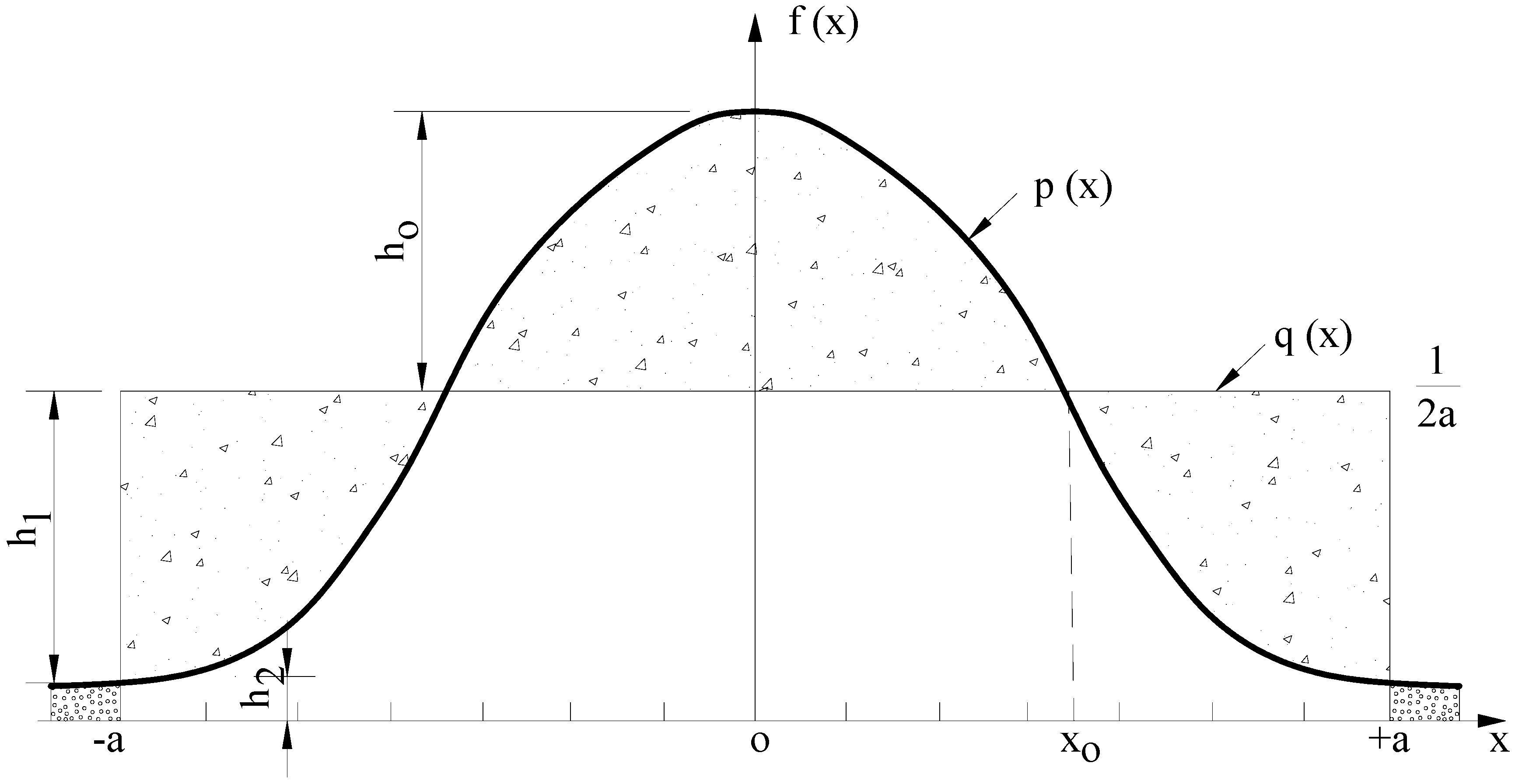
Let us assume that the a priori {
q(
x)} and a posteriori {
p(
x)} probability distribution functions of the random variable
X are known. If the ranges of possible values of the continuous variable
X are divided into
N discrete and infinitesimally small intervals of width Δx, the entropy expression for this continuous case can be given as:
The above expression describes the variation of information (or, indirectly, the uncertainty reduced by making observations) to replace the absolute measure of information content given in Equation (2). This definition is essentially in conformity with those given by Jaynes [
20] and Guiasu [
21] for continuous variables. When the same infinitesimally small class interval Δx is used for the a priori and a posteriori distribution functions, the term Δx drops out in the mathematical expression of marginal entropy in the continuous case. Thus, this approach eliminates the problems pertaining to the use of Δx discretizing class intervals involved in the previous definitions of informational entropy [
8,
10,
11,
12,
13].
At this point, the most important issue is the selection of a priori distribution. In case the process X is not observed at all, no information is available about it so that it is completely uncertain. In probability terms, this implies the selection of the uniform distribution. In other words, when no information exists about the variable X, the alternative events it may assume may be represented by equal probabilities or simply by the uniform probability distribution function.
If the a priori {
q(
x)} is assumed to be uniform, and a posteriori {
p(
x)} distribution of
X is assumed to be normal, the informational entropy
H(X/X*) can be expressed as:
By integrating Equation (14). The first three terms in this equation represent the marginal entropy of
X and the last term stands for the maximum entropy. Accordingly, the variation of information can be expressed simply as:
If the a posteriori distribution of
X is assumed to be lognormal, the informational entropy
H(
X/X*) becomes:
with and
and
being the mean and standard deviation of
If the a posteriori distribution of
X is assumed to be 2-parameter gamma distribution with parameters
α and
β,
The informational entropy
H(
X/X*) becomes:
where,
is the mean of the series,
α the shape parameter, and
β the scale parameter.
In the above, entropy as the variation of information measures the amount of uncertainty reduced by making observations when the a posteriori distribution is estimated.
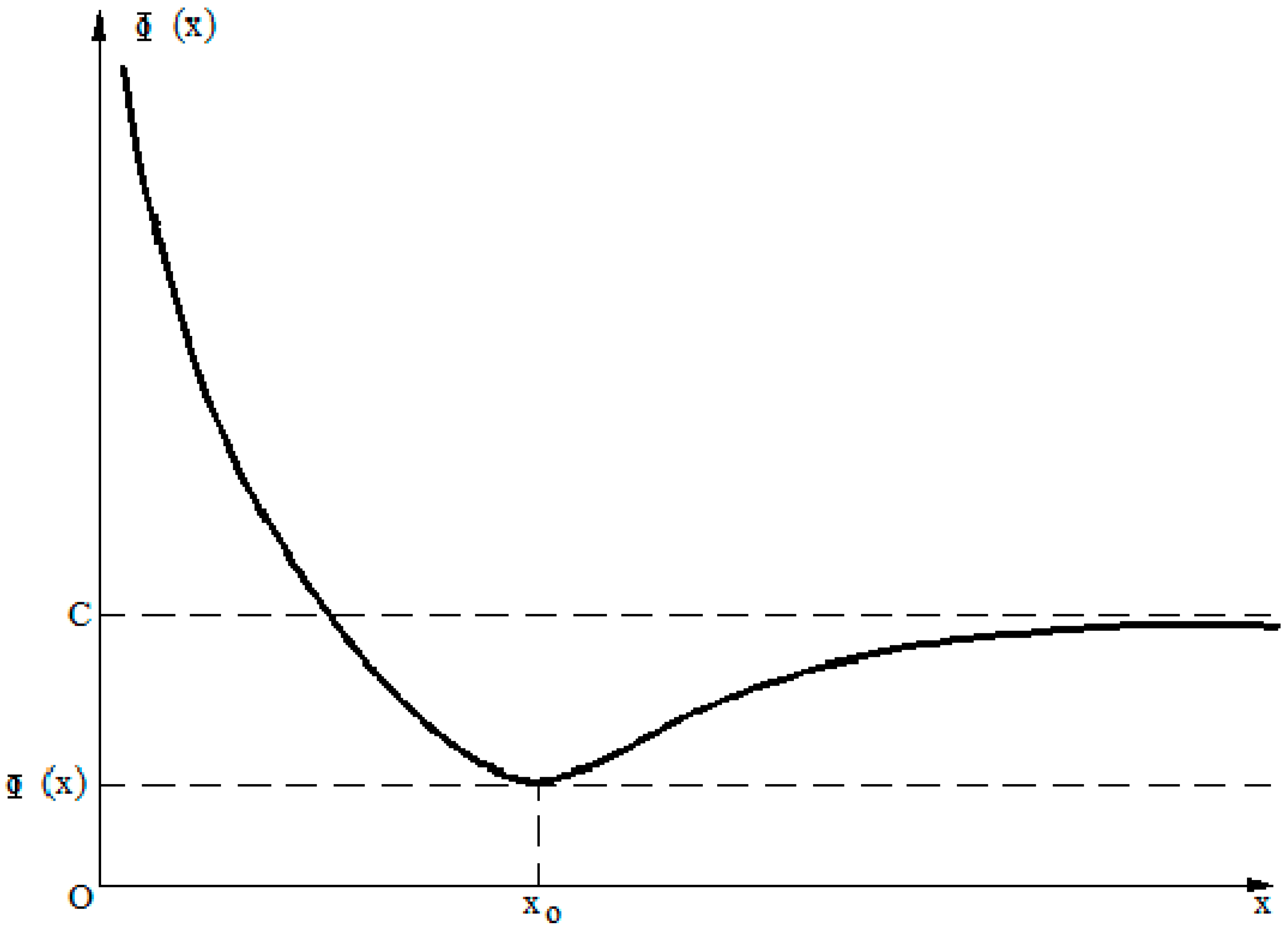
The maximum amount of information gained about the process X defined within the interval [a, b] is Hmax. Thus, the expression in Equation (16) will assume negative values. However, since H(X/X*) describes entropy as the variation of information, it is possible to consider the absolute value of this measure.
When the a posteriori probability distribution function is correctly estimated, the information gained about the random variable will increase as the number of observations increases. Thus, when this number goes to infinity, the entropy H(X/X*) will approach zero. In practice, it is not possible to obtain an infinite number of observations; rather, the availability of sufficient data is important. By using the entropy measure H(X/X*), it possible to evaluate the fitness of a particular distribution function to the random variable and to assess whether the available data convey sufficient information about the process.
5. Further Development of the Revised Definition of the Variation of Information
If the observed range [
a,
b] of the variable
X is considered also as the population value of the range,
R, of the variable, the maximum information content of the variable may be described as:
When the a posteriori distribution of the variable is assumed to be normal, the marginal entropy of
X becomes:
If the variable is actually normally distributed and if a sufficient number of observations are obtained, the entropy of Equation (16) will approach a value which can be considered to be within an acceptable region. This is the case where one may infer that sufficient information has been gained about the process.
When sufficient information is made available about
X, it will be possible to make the best estimates for the mean (
μ), variance (
σ), and the range (
R) of
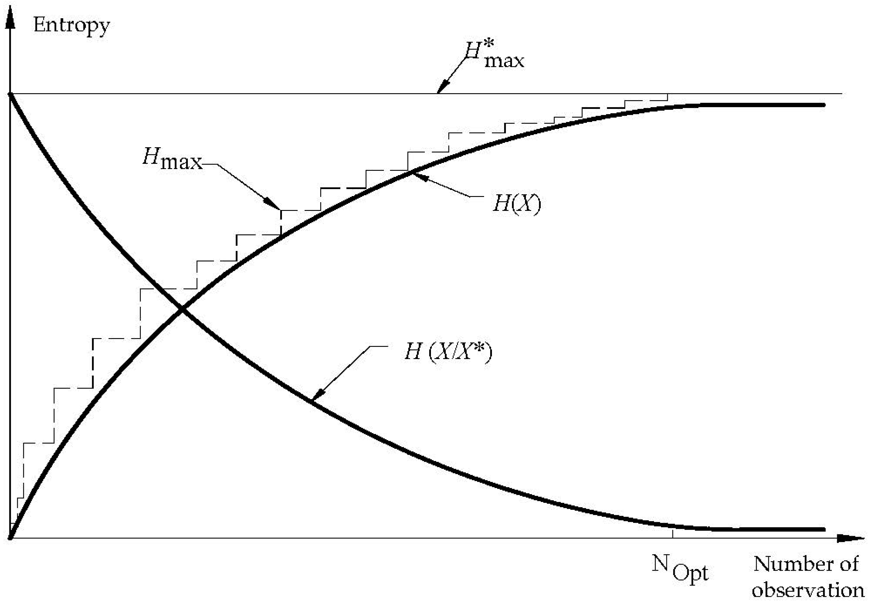
X. For this purpose, the variable has to be analyzed as an open series in the historic order. According to the approach used, the information gained about the process will continuously increase as the number of observations increase. Similarly,
Hmax and
H(
X) will also increase, while
H(
X/X*) will decrease. When the critical point is reached, where the variable can be described by its population parameters,
Hmax will approach a constant value;
H(
X) will also get closer to this value with
H(
X/X*) approaching a constant value of “
c” as in
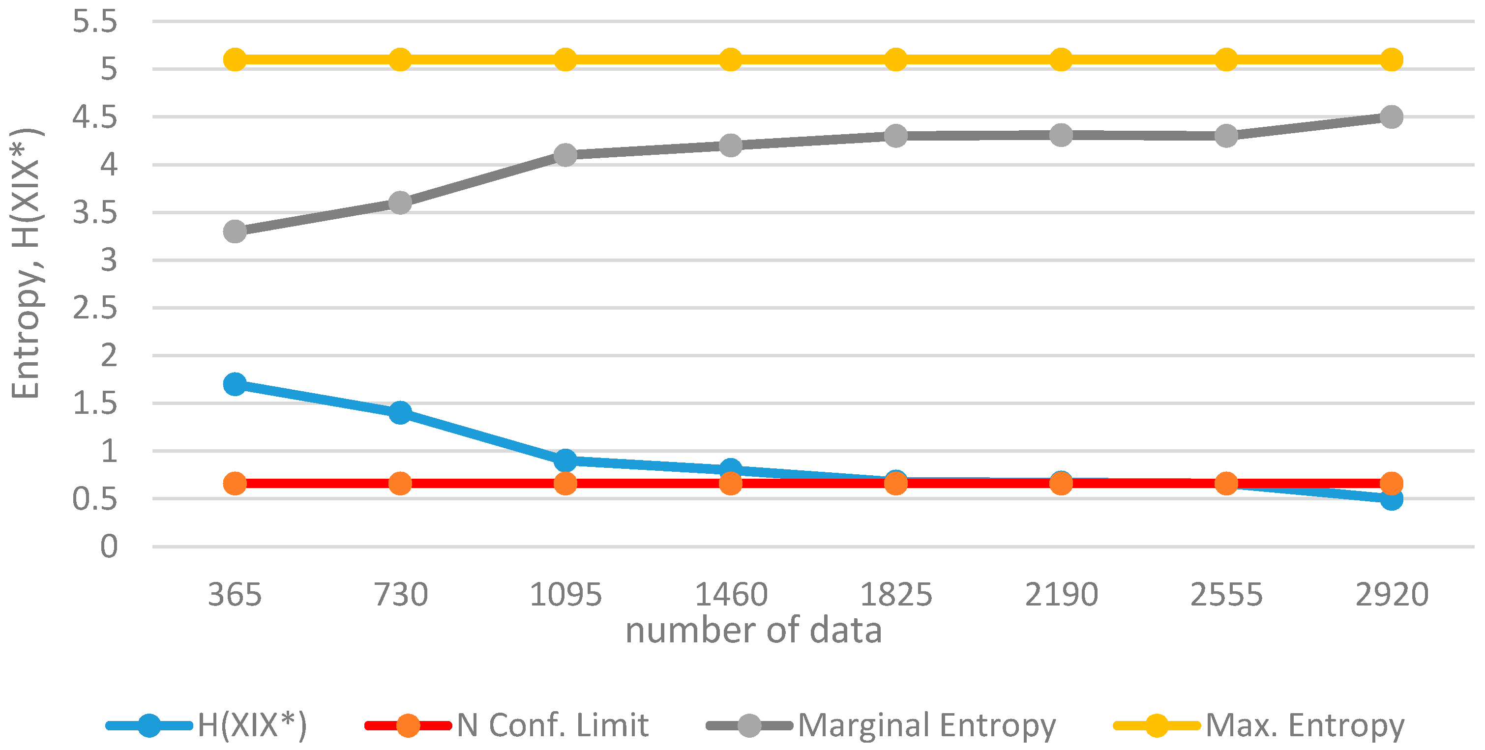
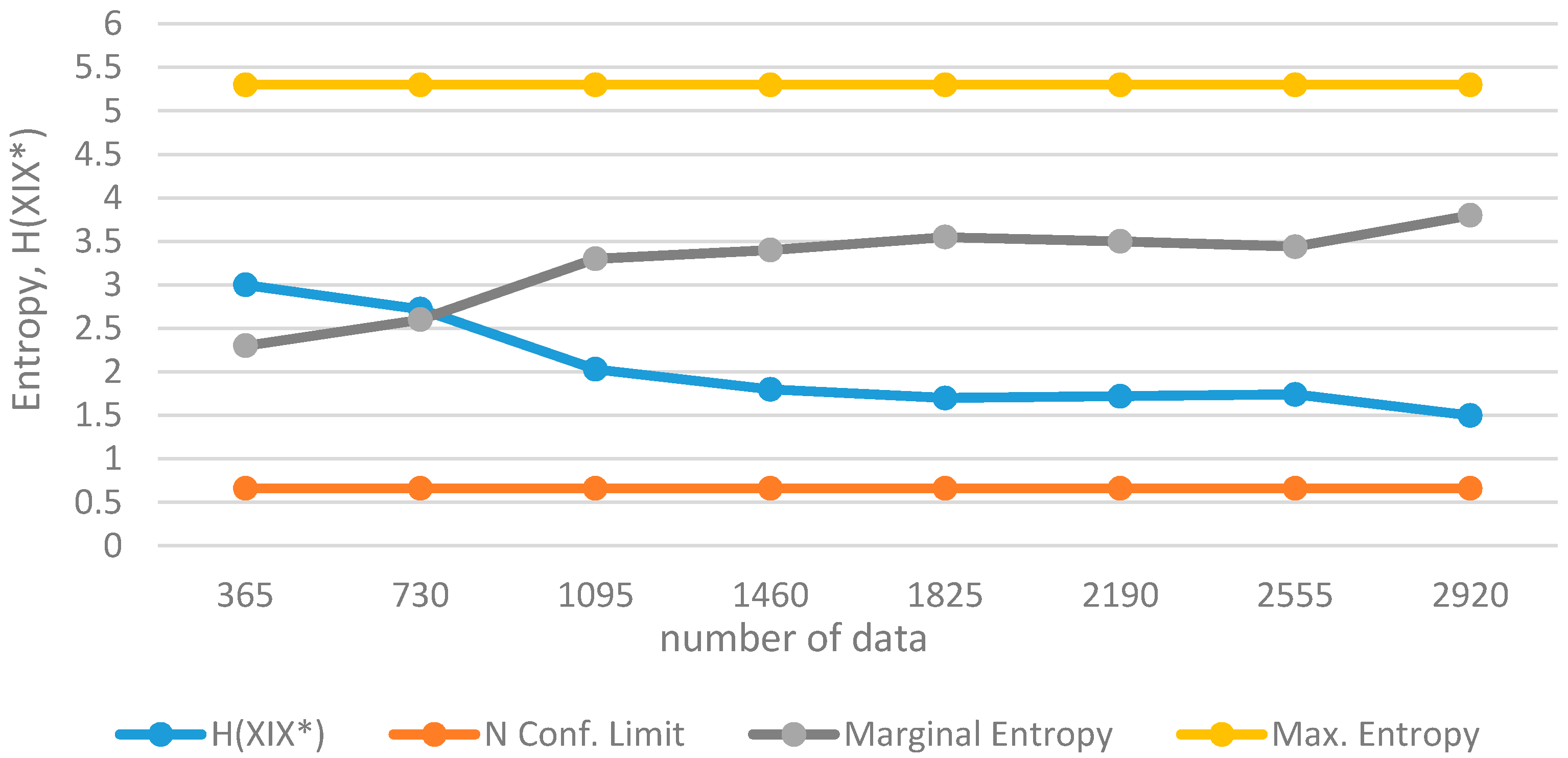
Figure 3.
Determination on Confidence Limits for Entropy Defined by Variation of Information
The confidence limits (
acceptable region) of entropy can be determined by using the a posteriori probability distribution functions. If the normal {
N(0,1)} probability density function is selected, the maximum entropy for the standard normal variable
z is;
with the range of
z being,
Here, the value
a describes the half-range of the variable. Then, the maximum entropy for variation
x with
N (
μ,
σ) is;
If the critical half-range value is foreseen as:
then the area under the normal curve may be approximated to be 1.
For the half-range value, replacing the appropriate values in Equation (16), one obtains the acceptable entropy value for the normal probability density function as:
using natural logarithms. When the entropy
H(
X/
X*) of the variable which is assumed to be normal remains below the above value, one may decide that the normal probability density function is acceptable and that a sufficient amount of information has been collected about the process.
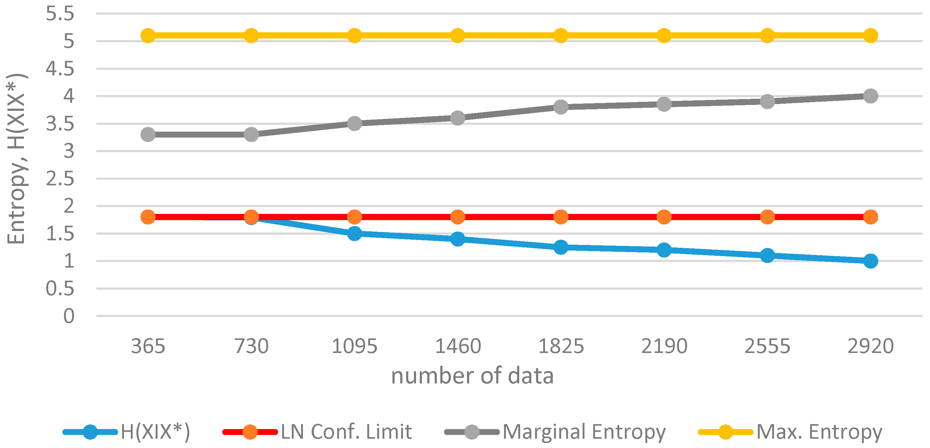
If the a posteriori distribution function is selected as lognormal LN(
μy,
σy), the variation of information for the variable
x can be determined as:
Here, since lognormal values will be positive, one may consider 0 ≤
x ≤ ∞. Then the acceptable value of
H(
X/
X*) for the lognormal distribution function will be;
According to Equation (40), no single constant value exists to describe the confidence limit for lognormal distribution. Even if the critical half-range is determined, the confidence limits will vary according to the variance of the variable. However, if the variance of x is known, the confidence limits can be computed.
7. Conclusions
The extension to the revised definition of informational entropy developed in this paper resolves further major mathematical difficulties associated with the assessment of uncertainty, and indirectly of information, contained in random variables. The description of informational entropy, not as an absolute measure of information but as a measure of the variation of information, has the following advantages:
- -
It eliminates the controversy associated with the mathematical definition of entropy for continuous probability distribution functions. This makes it possible to obtain a single value for the variation of information instead of several entropy values that vary with the selection of the discretizing interval when, in the former definitions of entropy for continuous distribution functions, discrete probabilities of hydrological events are estimated through relative class frequencies and discretizing intervals.
- -
The extension to the revised definition introduces confidence limits for the entropy function, which facilitates a comparison between the uncertainties of various hydrological processes with different scales of magnitude and different probability structures.
- -
Following from the above two advantages, it is further possible through the use of the concept of the variation of information to:
- ⚬
determine the contribution of each observation to information conveyed by data;
- ⚬
determine the probability distribution function which best fits the variable;
- ⚬
make decisions on station discontinuance.
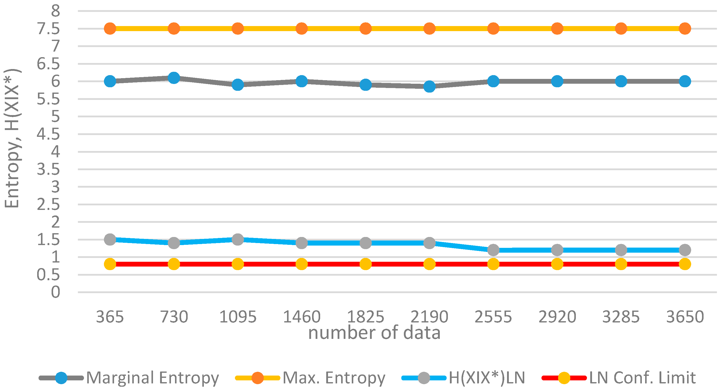
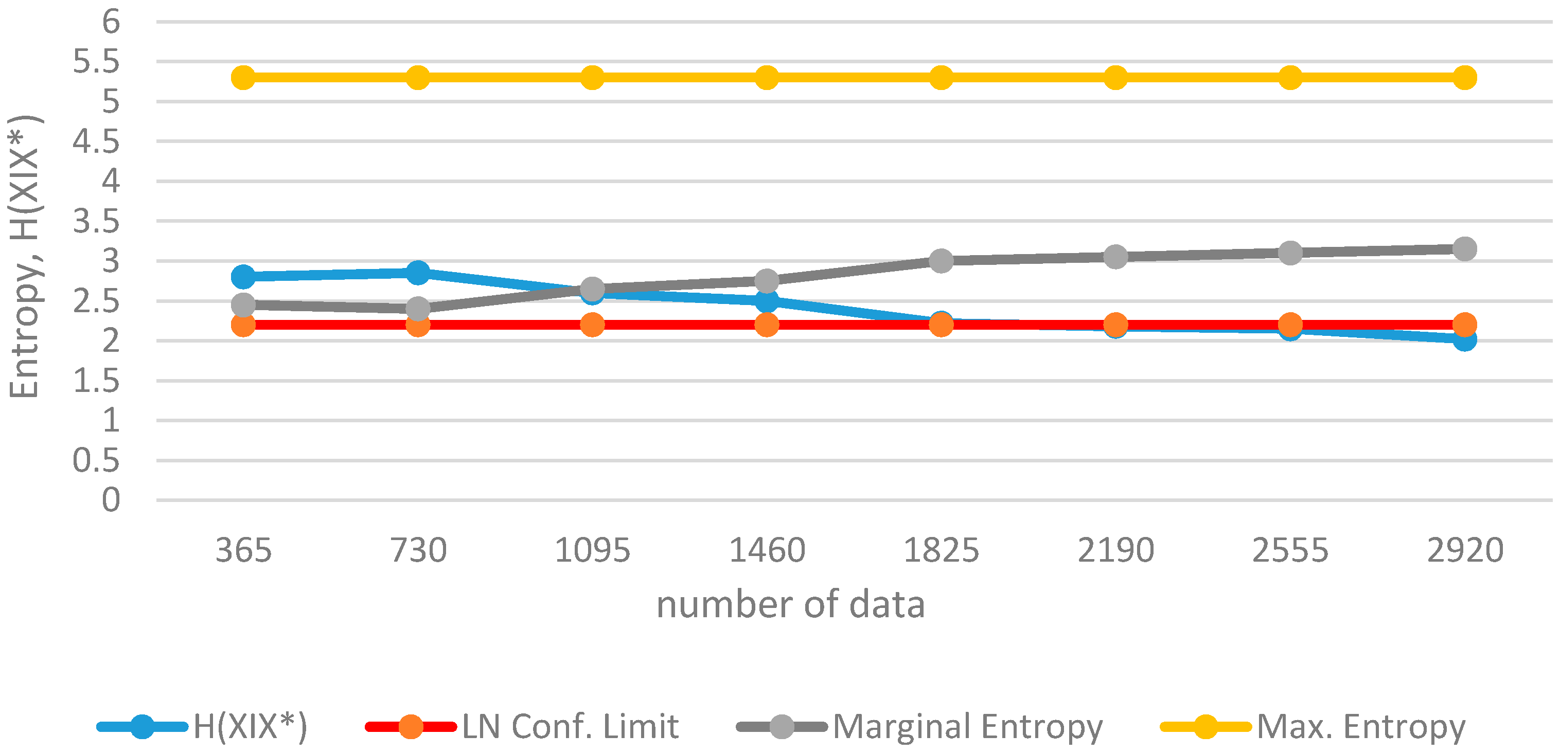
The present work focuses basically on the theoretical background for the extended definition of informational entropy. The methodology is then tested via applications to synthetically generated data and observed runoff data and is shown to give valid results. For real-case observed data, long duration series with sufficient length and quality are needed. Currently, studies are being continued by the authors on long series of runoff, precipitation and temperature data.
It follows from the above discussions that the use of the concept of variation of information and of confidence limits makes it possible to:
- -
determine the contribution of each observation to information conveyed by data;
- -
calculate the cost factors per information gained;
- -
determine the probability distribution function which best fits the variable;
- -
select the model which best describes the behavior of a random process;
- -
compare the uncertainties of variables with different probability density functions;
- -
make decisions on station discontinuance.
The above points are different problems to be solved by the concept of entropy, and further extensions of the methodology are required to address each of them.
