1. Introduction
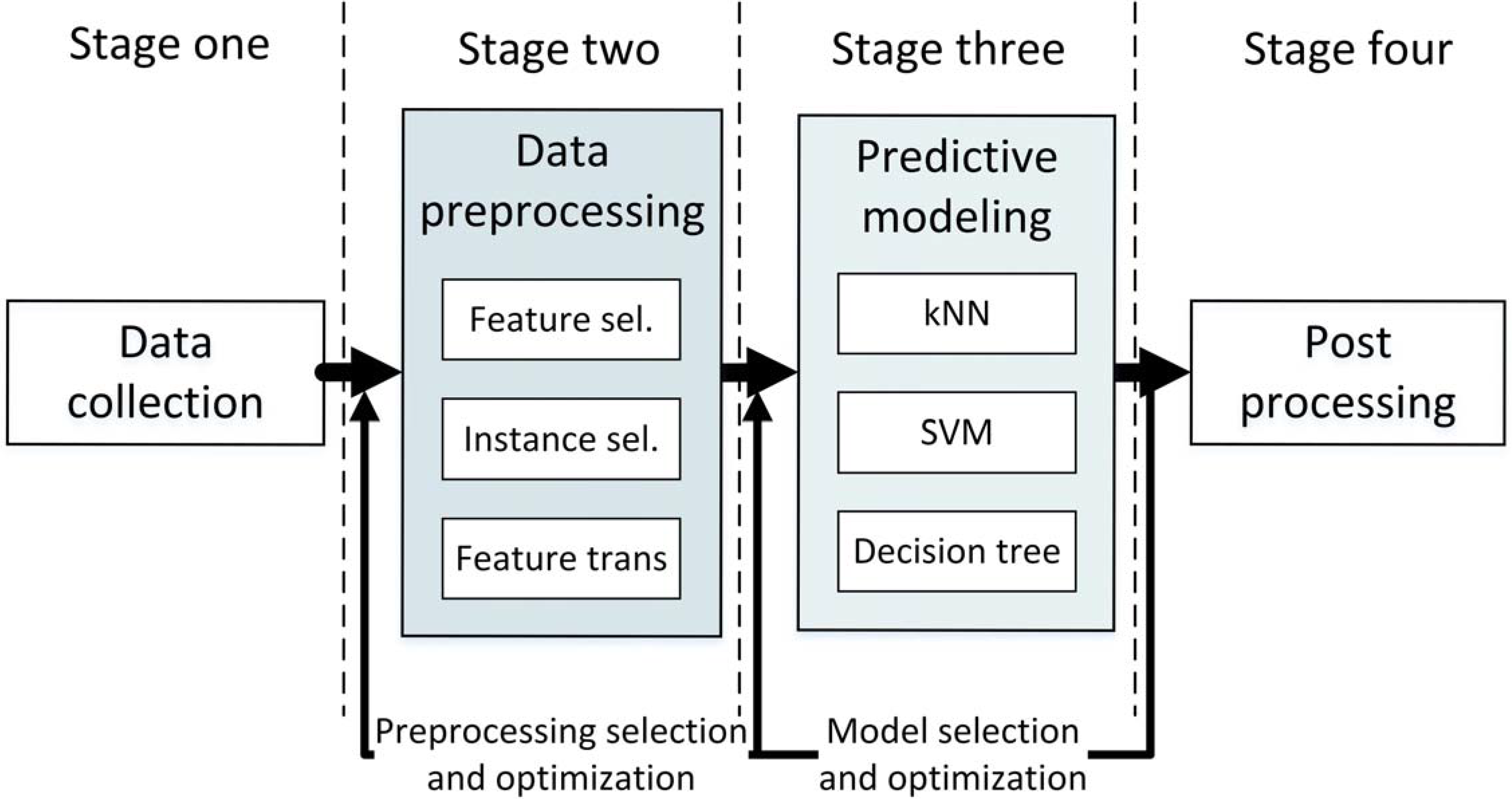
The data mining process consists of four stages, which are: (1) data collection; (2) data preprocessing (of all data transformation elements, for example feature normalization, instance or feature selection [
1], discretization [
2], and type conversion); (3) prediction model construction (e.g.,
k-nearest neighbors (
kNN), decision trees, and kernel methods) [
3]; and finally (4) data postprocessing (see
Figure 1). In real applications, when an accurate model is needed the process requires a search for the best combination among the elements available in stages (2) and (3). This significantly increases the computational complexity (we have to find the combination of preprocessing elements which best supports given prediction model) thus causing a rise in the expenses of building the prediction system and a longer computational time.
There are several solutions to this problem (for example [
4]), but one of the most robust solutions is meta-learning [
5], which is designed to accelerate stage (3). It is based on representing the training set, which consists of
n feature vectors by a single meta-date instance, and then uses it as an input to the meta-model which returns the estimate of the accuracy without training the actual (base) model [
6]. The obtained values for different base models are ranked from the best to the worst and only the best model with the highest estimated accuracy is finally trained on the entire training set.
The quality of the meta-learning system greatly depends on the quality of the meta-descriptors. In the beginning, these were simple statistics calculated per attribute or information theory measure (e.g., information gain) which can be obtained very quickly but usually are not very informative. Great progress was made with the introduction of landmark descriptors [
7]. They are based on performances obtained by simple and ”fast” algorithms like naive Bayes, decision trees, or one nearest neighbor (
1NN). These descriptors are very informative and provide important insights into the nature of the data, but on the other hand this radically increases computational complexity. The research to identify good data descriptors is still open and an overview is provided in
Section 3.
In this paper we also address this topic, but in contrast to the other researchers we postulate utilizing knowledge which can be extracted from the preprocessing stage, from the instance selection methods. These type of methods are commonly used for two purposes: data cleansing, and training set size reduction by eliminating redundant training samples. In other words, instance selection methods take as an input training set
and return a new dataset
such that
. In this paper we show that the relation between
and
is a very good landmark for the meta-learning system for example by considering the training set compression (see Equation (
1)). Intuitively, when the training set
can be significantly compacted, the classification problem should not be difficult. High classification accuracy should be easy to achieve, and in the opposite case, with low compression, the problem is expected to be difficult and low accuracy can be expected. An inverse relation appears for cleansing methods where the increase in compression corresponds to a deterioration of the accuracy. The main thesis of this paper that compression of selected instance selection methods is a good meta-data descriptor for estimating the accuracy of selected machine learning methods. Thus, we reuse information extracted from the preprocessing stage that was obtained without any computational effort, and use it to construct new landmarks.
As mentioned above, particular instance section methods were designed with different aims (cleansing, compression), so the relationship between and can reflect different properties of the training set. In order to validate this relation we examined a set of 11 instance selection methods and analyzed the relationship between compression and prediction accuracy. Having obtained the results we identify which algorithms can be used as landmarks for meta-learning. The study is based on empirical analysis on 80 datasets.
The paper is structured as follows. First, we discuss the state-of-the-art in instance selection and meta-learning, where the most popular algorithms are described in more detail, and then we show and discuss which and why particular evaluated instance selection methods are good landmarks. In
Section 5 we perform real-world experiments on meta-learning systems, and finally in
Section 6 we summarize the obtained results and draw further research directions.
2. The Instance Selection Methods
The purpose of the instance selection methods is to remove data samples. They take as an input the entire training set
consisting of
n samples (
,
,
, where
denotes
i-th symbol), and then eliminate from it useless samples, returning the remaining ones denoted as
. The difference between cardinality of the input dataset
n and the output dataset
, divided by the cardinality of the input dataset
n, is called compression.
Note that a approaching 1 represents a scenario in which , which means many samples are removed from the training set (we would call it high compression as is close to 1) and respectively when is close to 0 or in other words small compression appears when , that means just few instances were removed from .
In instance selection algorithms, the decision of selection or rejection of particular sample or samples is made by optimizing one of two or both objectives, which are:
Type-I: Maximization of the accuracy of the classifier. This objective is achieved by eliminating noise samples,
Type-II: Minimization of the execution time of the classifier. This objective is achieved by reducing the number of reference vectors, and keeping the selected subset of samples as small as possible by rejecting all redundant ones.
Note that this taxonomy is just one possible presentation (a more detailed view can be found in [
8]), however it is crucial as these two type of algorithms behave differently considering the relation between compression and prediction accuracy. An illustrative example of the accuracy–compression relation was presented in our preliminary paper [
9]. A theoretical background of sampling and instance selection derived from the information theory can be found in [
10].
In the paper we use and compare 11 instance selection algorithms, but for 2 of them additional configuration settings are used, so in total we have 13 methods to compare. This set of algorithms includes older ones like the condensed nearest neighbor rule (CNN) and the edited nearest neighbor (ENN) through to the decremental reduction optimization procedure (Drop) family developed at the end of the 1990s, to the more modern algorithms such as the modified selective subset (MSS). These are:
CNN [
11]. It is an ancestor of all condensation methods, and thus it belongs to the
Type-II group. It starts by randomly selecting one representative instance per class, and adds it to the reference set
(the dataset
remains unchanged while the algorithm works), and then starts the main loop where each misclassified instance from
by the nearest neighbor classifier trained on
is added to
. The algorithm stops when all the instances in
are correctly classified.
IB2. This was developed by Aha et al. as an instance-based learning [
12] algorithm (version 2). It is very similar to
CNN; it also starts by selecting one sample per class, adding it to
, but it only once iterates over all samples in the data, trying to add them to
if an instance is misclassified. It is also a representative of a
Type-II family.
Gabriel graph editing (
GGE) [
13]. This method builds a Gabriel graph over training data and then selects border samples and stores them in
. Border samples have at least one instance of another class in their neighborhood according to the Gabriel graph, and therefore this is a
Type-II method. The Gabriel graph is determined by validating condition
between every three instances, where
are instances from
, and
denotes the square of the
norm. However, there is is another known version of the Gabriel graph editing method, which keeps the remaining samples in
and the border samples are removed. In this case it works as a
Type-I method, being a regularization for
kNN. In the experiments we used the first approach, which keeps the border samples only.
Relative neighbor graph editing (
RNGE) [
13]. This method is very similar to
GGE . The difference is in the graph construction criteria, which is now defined as:
As shown in [
13], the following relation takes place:
where
is a set of
returned by given instance editing algorithm. The
are border instances according to the Voronoi diagram.
Edited nearest neighbor (
ENN) [
14]. This is another ancestor but for
Type-I methods, and it is often used as a preprocessing step before other instance selection algorithms. This algorithm analyzes the neighborhood of the given query instance
. If this instance is misclassified by its
k neighbors, it is removed from
. Initially
.
Repeated ENN (
RENN) [
15]. This method is an extension of the
ENN algorithm where the
ENN algorithm is repeated until no instance is removed (also a
Type-I method).
All-kNN [
15]. This is another extension of the
ENN algorithm (
Type-I method) where the
ENN step is repeated for a range of
values.
Drop n. The decremental reduction optimization procedure is a family of five similar algorithms [
16], which can be assigned to a mixture of
Type-I and
Type-II methods. It can be explained as dropping instances from
while at the beginning of the algorithm
.
Drop algorithms are based on the analysis of the associate array, which is defined as a set of indexes of instances having particular instance
in its neighborhood. In
Drop 1 the algorithm analyzes if the removal of instance
from the associates does not affect the classification accuracy, if so
is then removed. The
Drop 5 algorithm is similar to the
Drop 2 algorithm (thus only one was used in the experiments); again it analyzes the effect of the removal of
from the associates array, but in the analysis the order of removal becomes crucial as instances are ordered according to the distance to the so-called nearest enemy (the nearest vector from the opposite class) starting with the farthest instances first. The
Drop 3 and
Drop 4 algorithms are similar to
Drop 1 but before selection the
ENN algorithm is used to prune the dataset. These last two versions have not been used in the experiments; instead
Drop 1 and
Drop 5 were analyzed.
Iterative case filtering (
ICF) [
17]. This is a two-step algorithm. First, it applies the
ENN algorithm to prune noisy samples, then in the second step it finds a
local set for every instance
(
), defined by the largest hypersphere centered at
which includes only instances of the same class as
. The
local set is then used to calculate two statistics:
and if
then the sample
is removed from
.
ICF is another example of a mixed
Type-I and
Type-II method.
Modified selective subset (
MSS) [
18]. This is a modification of the selective subset algorithm proposed by Ritter [
19]. In the basic algorithm the authors define the so-called selective subset as a subset
, which is consistent (all samples in the training set
are correctly classified by the nearest neighbor rule based on
). Samples from the training set
must be closer to instances in
from the same class, and
must be as small as possible. The modified version applies changes to the definition of the selective subset, and selects examples which are closest to the nearest enemy of given sample. It belongs to the
Type-II family
A common strategy in the development of more recent instance selection algorithms is the assembly of both objectives into one algorithm, for example as in
noise removing based on minimal consistent set (NRMCS) [
20] or
class conditional instance selection (CCIS) [
21], or even in the
Drop s or
ICF, where first the noise filter is applied and then the condensation step starts. This usually results in a better and more consistent set of reference vectors being obtained, but as we will further show, these mixed type (
Type-I and
Type-II) methods negatively affect the relation between compression and prediction accuracy . For more details of classical instance selection methods and their comparison readers are referred to [
8,
22,
23,
24].
Instance selection methods are still under rapid development. Recent methods in the field first solve other problems and then use classification, namely, regression problems as in [
25,
26,
27,
28,
29,
30], instance selection in data streams as in [
31,
32,
33], and time series classification [
34,
35], or build ensembles of instance selection [
36,
37,
38,
39,
40] and even create meta-learning systems, which automatically adjust a proper instance selection method to a given dataset as in [
41,
42].
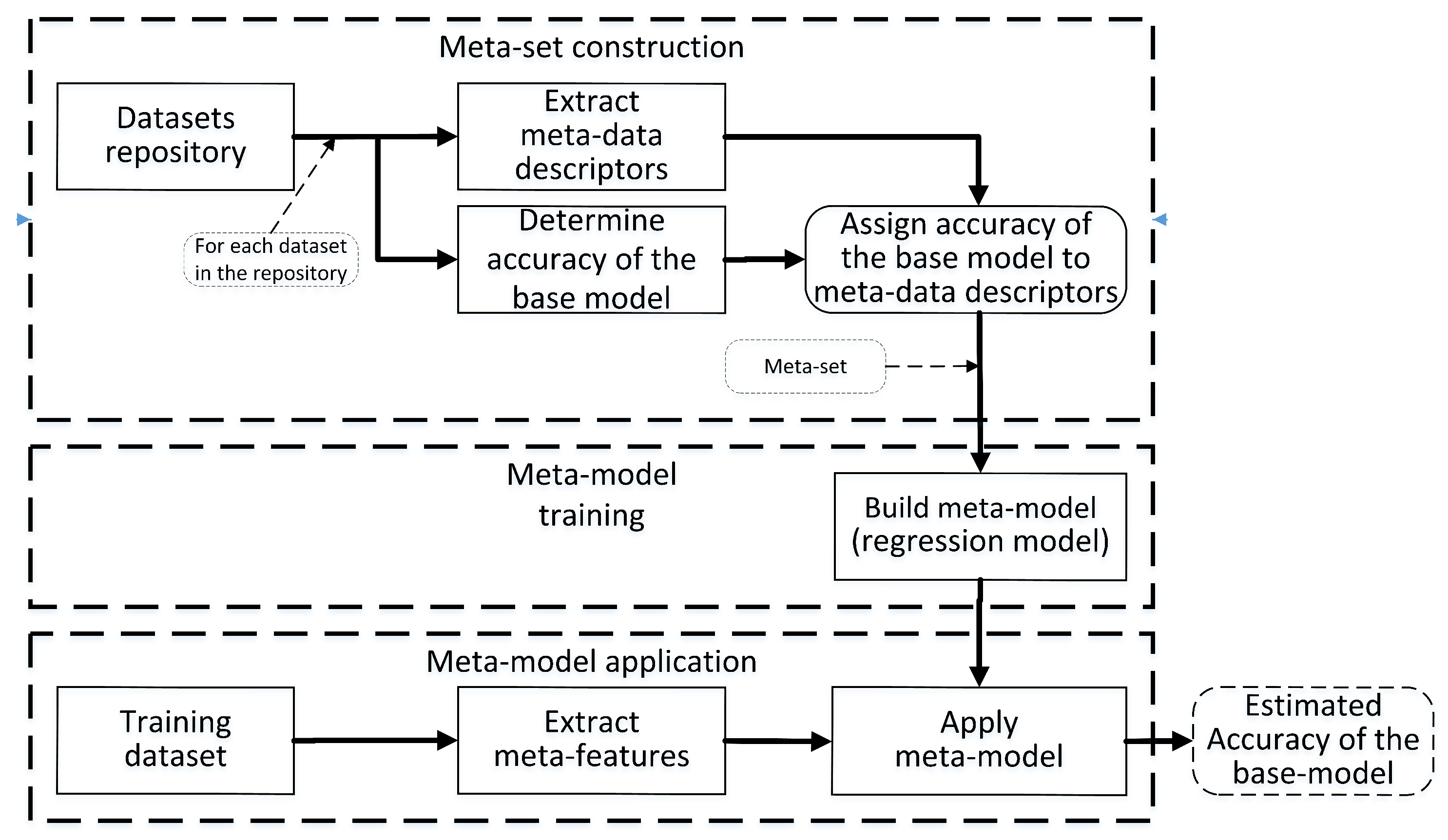
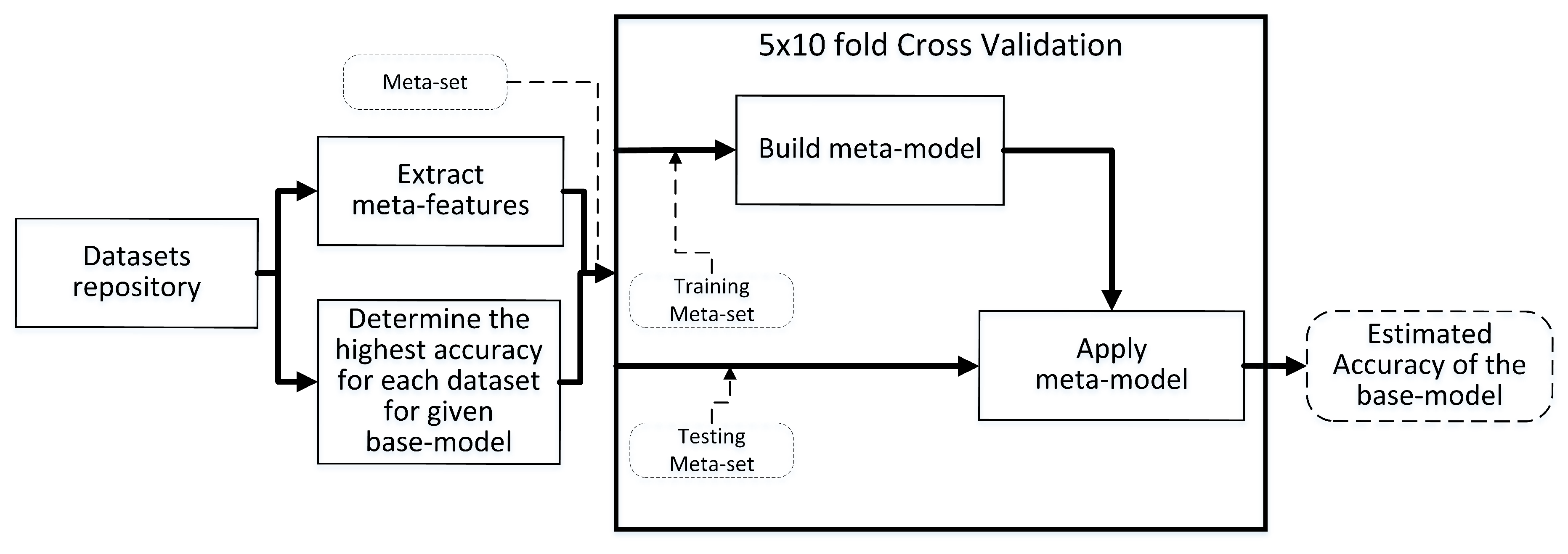
3. Meta-Learning
Meta-learning is the efficient selection of the best prediction model for a given training set
. In other words, it is a recommendation system which recommends a prediction model for a given training set. To achieve this goal, instead of validating each prediction model
M() (
base model) on training set
, meta-data descriptors are extracted from
, so that the training set is represented as a single instance of meta-data features and used by another previously trained meta-model (usually a classical regression model) which predicts the quality of
M() (the
meta-model application frame in
Figure 2). This significantly reduces the computational complexity, because to select the best model we do not need to train and optimize parameters of each
M(), and instead estimate its accuracy by using meta-data and the meta-model [
43]. Each meta-model is trained for a single base model using a meta-set (the
meta-model training frame in
Figure 2). Finally, the meta-set is obtained out of collection of historical datasets (a repository) for which we already know both the meta-date descriptors and the performance of the base model, so that each instance of the meta-set consists of both the meta-data extracted from given dataset, and a label representing highest accuracy of the base model (see the
meta-set construction frame in
Figure 2). In applications we need several meta-models, each dedicated to a specific base model, for example one for the support vector machine (SVM), one for
kNN, etc. The obtained estimated performances of the base models are then ranked and the best one is selected for final application. Another common approach replaces the regression-based meta-model with the
kNN model, which identifies the most similar dataset from the metaset (the nearest neighbors according to the meta-feature space), and returns an aggregated ranking of the best models obtained for each of the most similar datasets [
44]. In the experiments we follow the first approach.
In both approaches the quality of the meta-model strongly depends on selected meta-data descriptors also called meta-features, which should reflect the prediction power of given base model. Note that we need a separate meta-model for each base model. An extension of this approach even allows for the estimation of the value of hyper-parameters [
45] of the base model or at least helps to decide whether hyper-parameter optimization is needed [
46].
The problem is finding good meta-data descriptors which would allow us to accurately estimate the accuracy or other desired values like execution or training time, etc. The basic examples of meta-learning can be found in the
variable bias management system (VBMS) [
47] which automatically choses a learning algorithm based on two meta-parameters: the number of features and the number of vectors, often extended by descriptors representing the number of features of given type.
An extension of this idea is a meta-learning system which is based on a set of meta-variables describing aggregated statistical and information theory properties of individual attributes and class labels [
5,
6,
48,
49,
50]. Commonly reported meta-features of this type include: canonical correlation for the best single combination of features (called
cancor1), canonical correlation for the best single combination of features orthogonal to
cancor1, the first normalized eigenvalue of the canonical discriminant matrix, the second normalized eigenvalue of the canonical discriminant matrix, the mean kurtosis of attributes of
, the mean skewness of attributes of
, the mean mutual information of class and feature, joint entropy of a class variable and attribute, and entropy of classes, etc.
Another approach to determine valuable meta-data descriptors is the idea of landmarking [
7,
51]. It utilizes the relationship between the accuracies obtained by simple predictors with low computational complexity such as naive Bayes,
1NN, decision tree, and complex data mining algorithms like SVM, neural networks, or other systems. The selection of meta-features describing the dataset is the real challenge. Various authors use different combinations of landmarks and not only provide performance of the simple classifiers but also use model-based features where the structure of a simple model is provided as a dataset descriptor. A common solution is based on unpruned decision tree properties as described in [
52]. In this case, to represent the complexity of the data, authors suggested the ratio of the number of tree nodes to the number of attributes, the ratio of the number of tree nodes to the number of training instances, the average strength of support of each tree leaf, the difference in the gain-ratio between the attributes at the first splitting point of the tree building process, maximum depth, number of repeated nodes, a function of the probabilities of arriving at the various leaves given a random walk down the tree, the number of leaves divided by tree shape, and the number of identical multi-node subtrees repeated in the tree.
In [
53] the author studied a set of data complexity measures for classification problems to assess the accuracy. He divided these measures into three groups: Group 1 is comprised of measures of overlaps in feature values from different classes like the
maximum Fisher’s discriminant ratio and the
maximal (individual) feature efficiency; Group 2 refers to measures of separability of classes which include the
minimized sum of error distance by linear programming, the
error rate of linear classifier by linear programming, the
fraction of points on class boundary, the
fraction of points on the class boundary, and the
error rate of the 1 nearest neighbor classifier; and Group 3 contains measures of geometry, topology, and density of manifolds containing
nonlineality of linear classifiers by linear programming and the
fraction of points with associated adherence subsets retained. These measures are then compared using three artificially designed datasets and three classifiers:
kNN, C4.5, and SVM, and indicate which measure is suitable to which classifier. Recently, in [
54] authors suggested the generalization of meta-feature construction by defining a framework which covers all of already known meta-descriptors. It is based on defining three elements of the so-called objects: the source of meta-data (e.g., the dataset, the simple model, etc.); the meta-function (the element extracted from the object); and a post processing operation (the aggregation function). An integrated approach which joins all popular types of meta-features is available in the
Pattern Recognition Engineering (PaREn) system [
55] (recently renamed to MLWizard). It was used in the experiments discussed in
Section 5 as a reference solution (the list of meta-features extracted by PaREn is available in
Table 1).
In many cases we are not exactly interested in estimating prediction accuracy but rather in ranking the top classifiers. This problem was studied by Brazdil et al. [
44] who suggested use of a
kNN algorithm to naturally rank results according to distances in the meta-feature space. This approach was further extended. For example, Sun and Pfahringer proposed the forest of the approximate ranking tree which is trained on pairwise comparisons of the base models and the metaset [
56].
An alternative approach to meta-learning was proposed by Grąbczewski and Jankowski in [
57,
58]. It focuses on so called machine unification, such that the already-trained machines (a machine is a prediction model or data transformer) are cached and re-used when needed. This concept allows us to cache parts of the models and utilize them inside other complex machines. The proposed solution also ranks models according to the execution time such that the most promising machines are evaluated first. Note that this concept applies to both stages (2) and (3) of the data mining process.
For more details on meta-learning methods the readers are referred to [
59].
4. The Relationship between Dataset Compression and Prediction Accuracy
In
Section 2 we distinguished two basic types of instance selection objectives called
Type-I and
Type-II and also defined a third group constituting a mixture of these two. These types are important because the relation between compression and accuracy behaves differently. Considering
Type-I, for
kNN regularization methods, intuitively, when the dataset is clean without any noisy samples or outliers there is no need to remove any instances. The heuristics built into the algorithm may treat only some of the border instances as noise and remove them. As a result the compression is low. When the level of noise in the data increases (for example by mislabeling) or the decision boundary becomes jagged, the number of instances which are removed increases, and the compression grows. Now considering the prediction system, when the dataset is clean and the decision boundary is smooth and simple then the classification accuracy will be high. In the opposite situation the classification accuracy will drop, therefore intuitively we expect these two values (compression and accuracy) to remain in an inverse relation.
For
Type-II methods, which are aimed at compacting training data, when the decision boundary is smooth the dataset can be easily compacted and many instances can be removed, so the compression is then high. The noise in the data or a complex and jagged decision boundary reduce the compression as there are less regularities. In this case we expect an inverse relation in comparison to
Type-I methods, so increasing compression should reflect the increase in prediction accuracy. In [
9] we have evaluated this relation empirically on artificial and real-world datasets for
kNN classifier and two methods:
CNN and
ENN. Now we want to extend this work, and evaluate other more advanced instance selection methods which use more advanced heuristics to determine the final set
as discussed in the
Section 2. Note that some of the methods, such as the Drop family or ICF, combine both
Type-I and
Type-II. That means that the resulting compression rates may incorrectly reflect the complexity of the data set, since the relation between compression and accuracy for
Type-I and
Type-II remains in contradiction.
In order to solve this problem, we carried out a number of experiments on real-world datasets to verify which instance selection methods preserve strong correlation between compression and prediction accuracy. Because in instance selection applications two scenarios are possible (one in which the prediction model is trained on the entire training set without compression, and one in which the dataset used to train the predictor is already filtered by the instance selection), we evaluate both of them, and call them respectively Case A and Case B.
4.1. The Experimental Setup
Both experiments were carried out on 80 real-world datasets obtained from the Keel repository [
60] and UCI repository [
61]
Note that some of the datasets in both repositories have the same name but they have different content (different number of attributes or different number of instances). The
Src column in
Table 2 indicates the source repository of given dataset, and the datasets are also available in the
supplementary materials. In the study we compare 11 instance selection methods described in
Section 2 and for
Drop methods we also evaluated two additional parameters resulting in a total of 13 methods. The datasets used in the experiments represent a broad spectrum of classification problems from small ones such as
appendicitis which has 106 samples, up to larger ones such as the
shuttle dataset which has almost 58,000 samples. The datasets also contains different types of attributes, from simple, all-numerical features, through to mixed type features, to all-nominal features. The basic information about these datasets is provided in
Table 2, where the column
Src indicates the source of the dataset.
For all of the symbolic attributes in any dataset, the Value Difference Metric (VDM) [
62] was used, or more precisely, the heterogeneous version HVDM [
63], but instead of direct application of VDM metric each symbolic attribute
a was encoded on
c attributes (
c is the number class labels), where each new attribute represents conditional probability that the output class
given attribute
a has value
, where
is one of the symbols of attribute
a. As shown in [
64], this type of conversion is equivalent to the HVDM metric and is more accurate than the binary coding of symbolic attributes (the Hamming distance). After the feature type conversion, all attributes were normalized to the
range and then the 10-fold cross-validation test was used to evaluate the prediction accuracy.
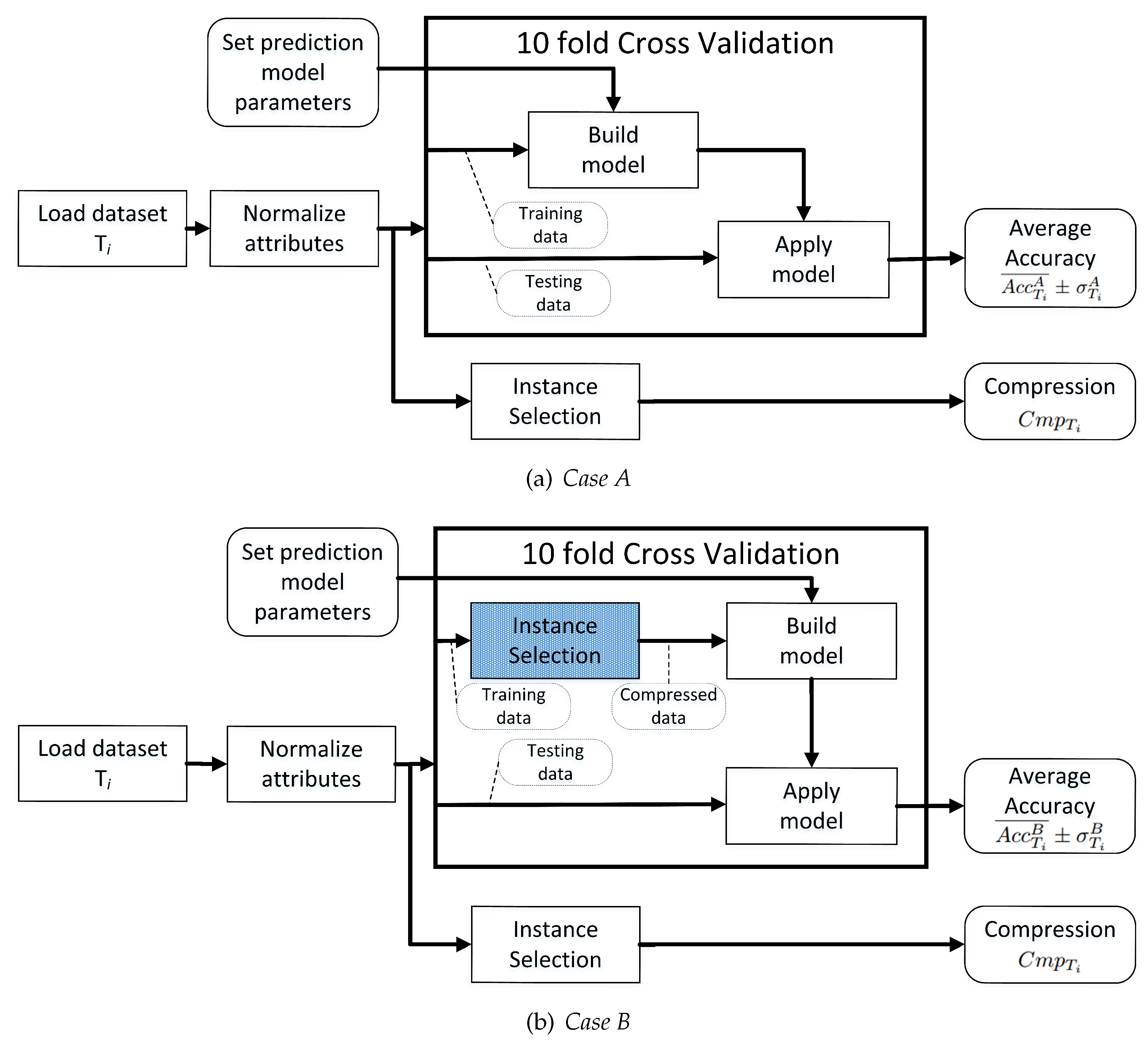
Earlier it was mentioned that the experiments were split into two scenarios. In the first one, denoted as
Case A presented in
Figure 3a, the instance selection was performed outside the cross-validation, and the prediction model was built on an uncompressed dataset such that instance selection did not affect the training set. This experiment mimics a real use-case where instance selection is executed once to estimate compression to assess the dataset properties and the cross-validation procedure is used to estimate the prediction accuracy of a given base model—a typical meta-learning scenario. Note that in all experiments hyper-parameters of instance selection were not optimized, and only the default values were used (see
Table 3), but the hyper-parameters of the prediction model were optimized to maximize prediction accuracy. For each setting of the classifier an independent model was built and only the best obtained results were recorded for the investigation.
The second experiment, called
Case B (presented in
Figure 3b), was aimed at repeating the previous one but in this case the prediction model was built using training set filtered out by the instance selection method. This experiment mimics a typical instance selection use-case where the prediction model is built on the dataset initially compressed by the instance selection algorithm. Again, hyper-parameters of instance selection were not tuned; only the prediction model was optimized to achieve the highest accuracy.
In all the conducted experiments all datasets were initially randomly divided into 10 subsets (preserving class frequency—a so-called stratified sampling) and these subsets were used in the cross-validation test.
In the experiments the state-of-the-art and the most robust and commonly used prediction models were used, such as SVM [
65,
66,
67] and random forest [
68,
69,
70], as well as the
kNN model. All the experiments were executed using RapidMiner software as a shell system [
71]. Instance selection was performed with the
Information Selection extension [
72] developed by the author, which includes the
Instance Selection Weka plug-in created by Arnaiz-González and García-Osorio [
26]. The SVM implementation was based on LibSVM library, and random forest was used from the Weka suite. For each prediction model the meta parameters such as
k for
kNN,
C and
for SVM, and number of trees of random forest were optimized using the greed procedure. In the final results only the highest average accuracy was reported. Hyperparameters evaluated in the experiments are shown in
Table 4, and RapidMiner processes representing the experiments are available in
supplementary materials.
4.2. Compression-Accuracy Relation for the Case A Scenario
As stated in the previous section,
Case A assumes that compression and prediction accuracy are evaluated independently, and the goal of the experiments is to verify a typical meta-learning use-case where compression is used as a landmark and does not affect the training set. For that purpose for each of the datasets presented in
Table 2, compression as well as prediction accuracy were measured (labeled respectively as
and
, where
denotes
i’th dataset, and the
A superscript is used to distinguish the values recorded in
Case A). The experimental process is described in the scheme presented in
Figure 3a and the results were collected for all instance selection methods and the all above-described classifiers.
To measure the relation between
and
we used three different measures. These were the Pearsons correlation coefficient
, root- mean-square error (RMSE) of the linear model, and the coefficient of determination (
) of the same model. The correlation measure was evaluated with a confidence level of 0.05, and results are shown in
Table 5.
These results indicate that compression is significantly correlated with accuracy, at least for the majority of the analyzed compression methods. For the four methods CNN, IB2, ENN, and RENN the absolute value of correlation for all classifiers is above . For one it is almost 0.9 (the All-kNN), and for the remaining ones it is above 0.5. The exception is ICF, for which the correlation is very low and close to 0. The ENN, RENN, All-kNN, and ICF have negative values of correlation coefficients, and this is consistent with the above-described interpretation of Type-I and Type-II methods.
Likewise, the other measures show similar behavior, although the RMSE between the true and the estimated accuracy clearly indicates that for half of the instance selection methods (Drop, RNGE, GGE and ICF) the error is almost four times higher compared to the best result. Also noticeable is the difference between the RMSE obtained when estimating the accuracy of the kNN classifier and the remaining base-models, where the RMSE is approximately 1.7 times smaller than the RMSE and RMSE. Also, the measure drops by 10% between best results obtained for kNN and the other classifiers. This is reasonable as instance selection methods internally use kNN to determine which instances should be removed or kept, so that it better reflects the performance of kNN classifier.
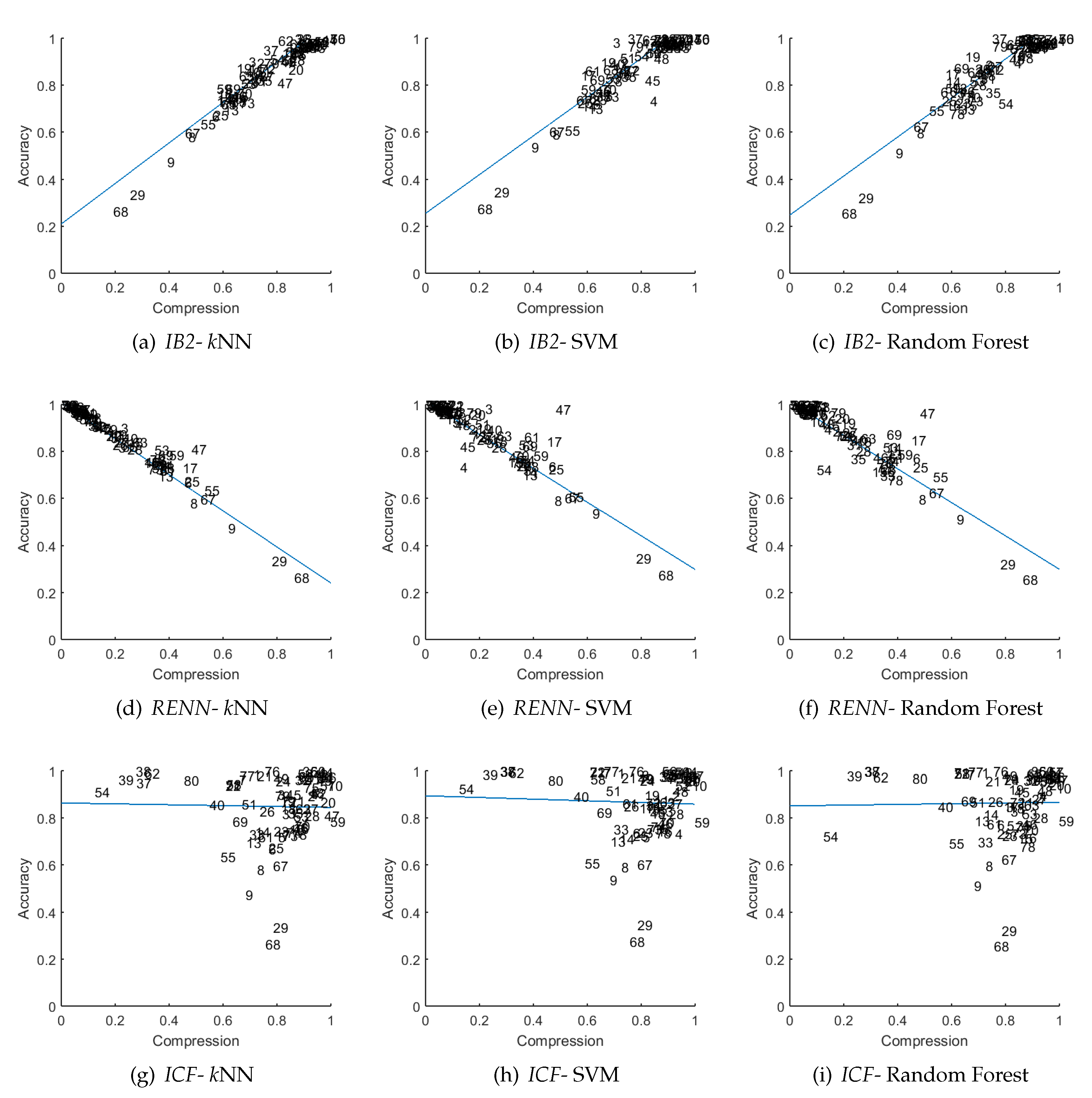
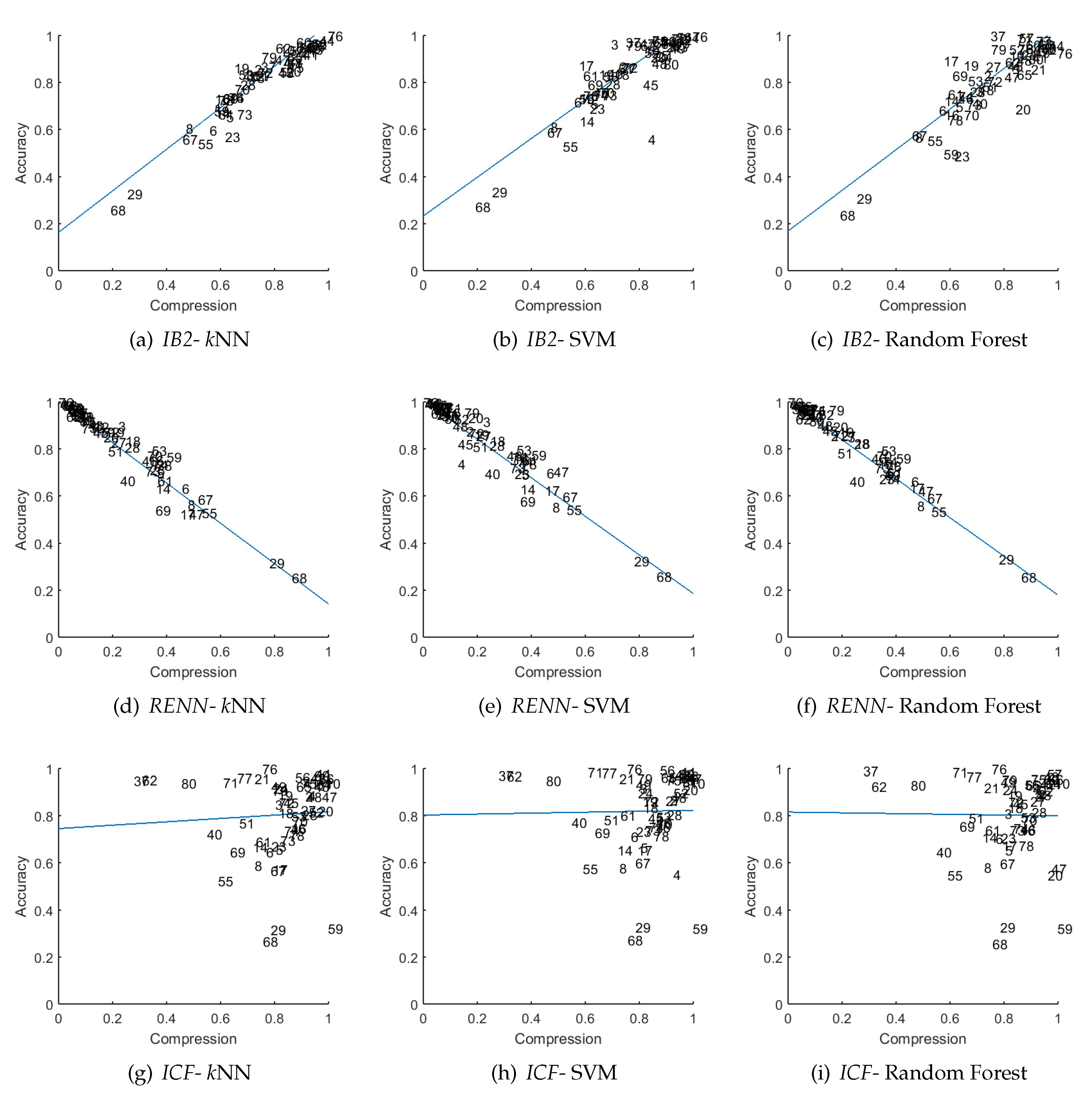
Of the collected results for three instance selection methods:
RENN,
IB2 and
ICF, we drew figures representing the
-
relation (see
Figure 4). These methods represent the highest correlation for the
Type-I method, the highest correlation for the
Type-II method, and the worst results. In the figures the X-axis represents
and the Y-axis represents
; each data-point is marked with a number
i and represents a pair of
obtained for
i-th dataset (see ID column in
Table 2). The blue line shows the linear regression (LR) model
for which the RMSE and
were measured.
The first two rows of
Figure 4 confirm a strong linear relation between accuracy and compression. Interestingly, comparing results of
IB2 and
RENN for SVM (but also for random forest) some of the outlying data points represent different datasets. For example, in
Figure 4e the most outlying dataset is number 47 which is not easy to recognize (it is almost in line with the others) in
Figure 4b. This property is desired, as compression of these two methods partially complements each other.
The third row shows the
ICF compression in relation to the performance of the classifiers. Here we can not see any relation; the data points are randomly distributed around (1,1) coordinates. For some datasets which have a very low compression we observe a very high performance (for example for the
spectrometer dataset (
)). Also, for datasets for which compression is high, the performance is very low (as for the
marketing (
) or
abalon datasets (ID
)). The explanation of these results will be presented in
Section 4.4.
4.3. Compression–Accuracy Relation for the Case B Scenario
The
Case B experiment (
Figure 3b) was designed to evaluate the compression–accuracy relation for scenario where the prediction model is built on a compressed dataset. In this case the experiment returned an average accuracy denoted as
(here we use the
B superscript to distinguish accuracy obtained in this scenarios) and compression
. The results are presented in the identical form to
Case A and the same quality measures are used (see
Table 6). The main difference is in the accuracy of classifiers. The RMSE,
, and the correlation
r were calculated between
. Note that in
Case B we used compression identical to that used in
Case A (calculated in
Case A, hence without cross-validation), to make the results of
Case A and
Case B comparable.
Again, the obtained results indicate a significant relationship between compression and accuracy, but not in all of the cases, as in
Case A. The strongest relationship was observed for the same methods, which are:
CNN,
IB2,
ENN,
RENN, and
All-kNN. The other methods have also similar values; only the correlation sign of
ICF changed, but this may be a result of numerical artifacts because the value is also close to 0. The plots are also presented for
RENN,
IB2, and
ICF to make them comparable to the previous results. Obtained results are shown in
Figure 5, where each row represents an individual instance selection algorithm, columns represent different classifiers, and the blue line in each plot is the linear regression model.
The plots are very similar to those of Case A. Again, the compression of Type-I (ENN, RENN, All-kNN) methods shows a linear relation to the accuracy, and increasing compression leads to a drop in accuracy. For Type-II methods (CNN, IB2, GGE, RNGE, MSS), an increase of compression correlates with an increase of accuracy. The mixture methods such as the Drop family or ICF do both, and display low correlation.
Comparing results from
Case A and
Case B, especially for the SVM and random forest, in
Case B we observe a smaller RMSE, and higher
and correlation values. This results from the dataset compression process which adjusted the datasets to the
kNN classifier. For example, this can be observed for the dataset with ID 47, which is in line in
Figure 5e of
Case B, while in
Case A (
Figure 4e) it significantly increases the error.
4.4. Discussion of the Results Obtained in Case A and Case B
In the previous sections we indicated that ENN RENN and All-kNN are representative of Type-I methods and for all of them we recorded very high levels of correlation between accuracy and compression. The minus sign of the correlation indicates that compression is inversely proportional to the accuracy, and this phenomenon was explained in the beginning of this chapter. The RENN and All-kNN are modifications of the basic ENN algorithm, so it is not surprising that all these methods behave similarly. The analysis of the code of ENN algorithm points out that its compression is equivalent to the leave-one-out estimation of the error rate of the kNN () classifier, as all incorrectly classified samples by kNN () are removed.
The
RENN method repeats the
ENN procedure until no instance is removed, so it often removes more samples than the basic
ENN procedure. This imitates to some extent the
kNN classifier with higher values of
k (see
Table 4), which explains why the correlation of
RENN is higher than the one of
ENN. The
All-kNN rule also repeats the
ENN step, but for a set of
values (these settings were used in our calculations). Thus, it could not reflect as accurately the performance of the
kNN classifier. It becomes especially noticeable when the best performance is obtained for large
k (
or
). Considering the computational complexity of these three algorithms where the
ENN has the lowest (
), followed by
All-kNN, and the complexity of
RENN reaches
, the last two are definitely too high for the requirements of meta-learning systems. In this case we recommend the use of
ENN instance selection as a landmark.
In case of condensation methods (
Type-II) we analyzed the
CNN,
IB2,
RNGE,
GGE and
MSS algorithms. The highest level of relation was obtained for
IB2 and
CNN, which are very similar algorithms. In
CNN the
IB2 procedure is repeated until all samples of the training set
are correctly classified by the 1NN classifier trained on
. Hence, it uses the resubstitution error to determine
. In other words, both these methods try to maintain the performance of 1NN classifier but we can not give any simple intuitive explanation as to why compression of these two methods is so significantly correlated to the prediction accuracy of the classifiers. The
GGE and
RNGE methods keep the border instances but using different criteria, as described in
Section 2. The compression of these methods directly reflects the complexity of the decision boundary, or indicates how many instances have a neighbor from the opposite class. These types of measures were also discussed and analyzed by Cano in [
53] who distinguished a special type in his analysis called
Fraction of Points on Class Boundary, but unlike our analysis he used a minimum spanning tree to distinguish the fraction of border samples. He indicated that this type of measure has a
clear relation with classifier performance. We also noticed this property but in our analysis the compression of
IB2 and
CNN were much more informative than the number of border samples. With respect to
IB2 and
CNN, the the former algorithm is more favorable, as it has higher correlation and lower computational complexity, which in the worst case can reach
.
The Drop family as well as ICF did not reach such significant results. They are both designed to perform dataset cleansing as well as a condensation procedure. The compression does not reflect correctly the accuracy, because these two procedures are contradictory, as the cleansing methods have a high negative correlation while the condensation methods have a positive correlation. This is especially significant for the ICF algorithm, which directly applies the ENN algorithm (for which small compression corresponds to high accuracy) before condensation (high accuracy corresponds to high compression) which results in correlation almost equal to 0. In Drop the condensation dominates so it has positive correlation. The computational complexity of these two methods is also very high, reaching so it also limits their possible applications to meta-learning.
5. Meta-Learning Applications Using Compression-Based Meta-Data
Previous experiments were focused on the analysis of individual relation between compression and accuracy for each instance selection method and classifier. The obtained results pointed out some limitations, which are related on one hand to a low correlation between compression and accuracy as in ICF, and on the other hand to computational complexity issues. Now, the question arises as to how compression-based meta-features work in real meta-learning problems. For this purpose we conducted another set of experiments as described below.
5.1. Experiment Setup
The experiments were designed to investigate the impact of the compression-based meta-features on the prediction quality of the meta-model. For that purpose four sets of meta-features were designed:
- Set 1
State-of-the-art descriptors. This is the reference solution, which consists of 54 meta-features described in detail in
Table 1.
- Set 2
Compression-based descriptors. These include the compression of all instance selection methods, in total 13 meta-features.
- Set 3
Compression-based descriptors. These include only the compression of the two methods suggested in the previous section, namely ENN and IB2.
- Set 1+3
Combination of Set 1 and Set 3 descriptors. These are descriptors described in Set 1 and Set 3 to analyze the influence of compression-based meta-features on the state-of-the-art solution.
These sets on one hand provide a base rate, Set 1, and on the other hand analyze various scenarios of applications of compression-based meta-features.
The meta-model used in the experiments should take into account two properties:
it should be an accurate nonlinear regression model, which can be applied to each of the metasets.
it should return the feature importance indicator which would allow for assessment of the impact of each of the meta-features on the final results.
In order to satisfy the above properties we used bagging of the regression trees implemented in the Matlab Statistical and Machine Learning Toolbox. It is a very accurate regression model, which takes advantage of the regression trees, for which the feature importance index can be easily calculated. It is obtained by summing changes in the mean squared error resulting from the splits on every attribute, and dividing the sum by the number of branch nodes. The final index is aggregated over the ensemble.
The scheme of the experiments follows the one presented in
Figure 2, except that it is embedded into the five times-repeated 10-fold cross-validation process. The detailed view of the test procedure is shown in
Figure 6. The process starts by creating the metaset using 80 datasets described in
Table 2. First for each of the datasets contained in the repository meat-features are extracted and every new meta-instance is labeled with the highest accuracy obtained for a given base-model (the so-called true performance). Then starts the five-times repeated cross-validation procedure which returns the root-mean-square error (RMSE). The error is calculated between the performance obtained for a given dataset contained in the repository estimated before the cross-validation procedure (the true performance) and the one returned by the meta-model. In the experiments we used the same set of the base-models which were used in the previous experiments, namely
kNN, SVM, and random forest, with the same parameter settings (see
Table 4). In total the process was executed 12 times (4 sets of descriptors × 3 types of base classifiers). Finally, the obtained results were evaluated using paired
t-test to verify statistical significance of the difference between the results obtained from the reference
Set 1 and the remaining sets of descriptors containing compression-based meta-features. The default significance level (
) was used.
5.2. Results and Discussion
The obtained results presenting the minimum RMSE of the meta-model are shown in
Table 7. The best results are marked in bold, and next to the results the
p-value of the statistical test is reported.
The error rates indicate that the most accurate metasets according to the meta-model are those containing compression-based meta-features, which in all cases performed significantly better than the reference Set 1. Among metasets comprising compression-based descriptors, for the kNN classifier the most accurate system was obtained for Set 2. It is not surprising as the instance selection methods internally use the kNN classifier. The second most accurate system was obtained for Set 3 and the third was obtained for Set 1+3. Similar results are obtained for SVM, here again the best set is Set 2 followed by Set 3 and Set 1+3, but the difference between Set 2 and Set 3 is very small. For random forest, the situation changes, and now the best is Set 1+3, in second place is Set 2, and Set 3 takes third place.
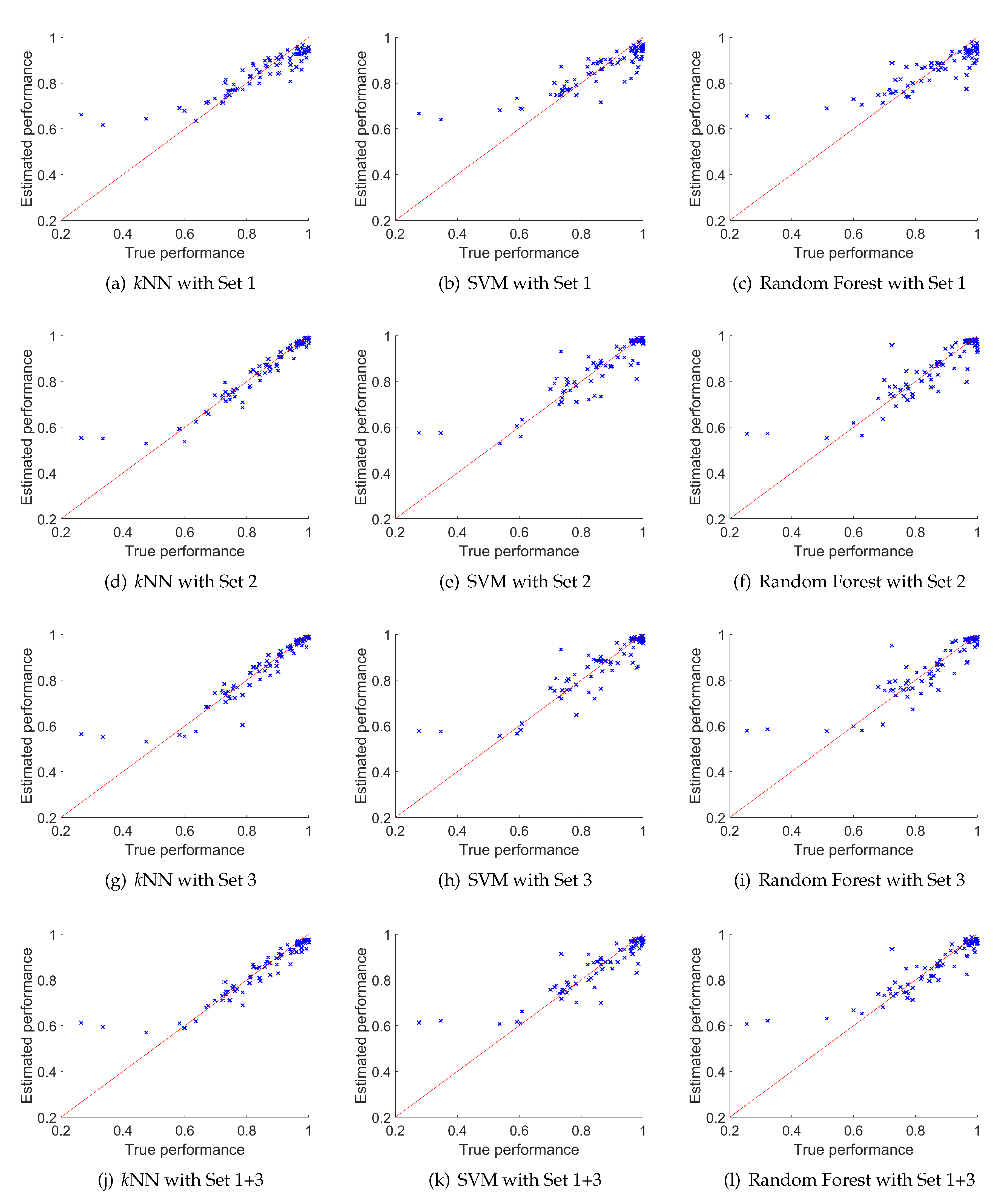
The detailed view of the obtained results (from the five-times repeated cross-validation procedure) is also plotted in
Figure 7. It shows 12 plots, where each represents performance estimated from the meta-model as a function of true performance for each of the 80 datasets denoted using the
x mark (these values are averaged over five runs of cross-validation tests). The rows of
Figure 7 represent results obtained for meta-model trained using different metasets. They are, respectively, row 1:
Set 1; row 2:
Set 2; row 3:
Set 3; and row 4:
Set 1+3. Columns represent different base classifiers, column 1:
kNN ; column 2: SVM; and column 3: random forest.
These results indicate that for all base classifiers every meta-model overestimates results for the datasets with poor accuracy (below 60%), but this effect is less apparent for datasets containing compression-based meta-descriptors where the estimated performances are closer to the red line. Similarly, for high performances (close to 1) for all base classifiers trained on Set 1 (first row) the performance is underestimated—see the blue cloud of points close to coordinates which are under the red line. This effect does not appear for the remaining rows, that is for metasets containing compression-based meta-features. The red line in the plots indicates perfect match between true and estimated performances.
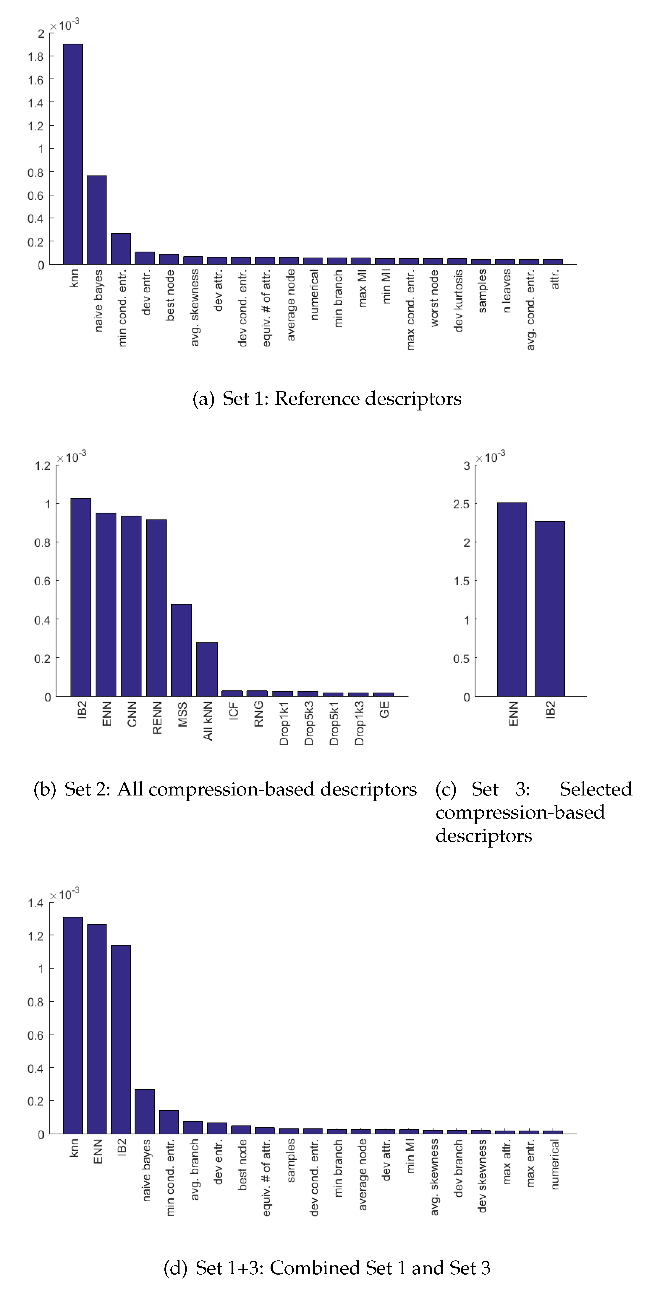
To analyze which of the meta-features are the most significant for the meta-model we trained 12 meta-models (for each metaset and for each classifier) on the entire metaset (without splitting the training and test part), then we extracted the feature importance index. The indexes were then aggregated by averaging their values and plotted, as a result of which we obtained one figure per metaset (see
Figure 8). The averaging process was required because for
Set 1 and
Set 1+3 we noticed small changes in order according to the classifier, such that, for example, for SVM the
dev. attr. <
avg. skewness and for
kNN the opposite relation occurred with
dev. attr. >
avg. skewness without significant differences in the value of the indicators. For
Set 1 and
Set 1+3 only the top 22 features were shown in figures to make it readable.
Meta-feature importance indicators gathered for Set 1 point out that the most valuable attribute is the performance of kNN, which is over two times more important than the naive Bayes-based landmark and over six times more important than the minimal conditional entropy. For Set 2 the most important were compressions obtained by IB2, ENN, CNN, and RENN which had approximately equal indexes, followed by MSS and All-kNN. The remaining ones have indicators very close to 0. Note that Set 2 was used just for comparison, and because of computational complexity it is not applicable ina real live scenario, despite the fact that it allowed the best results for kNN and SVM.
In case of Set 3, both meta-features were almost equally important. Finally, for the Set 1+3 the indexes for kNN, ENN, and IB2 were all the most important, followed by naive Bayes, which had a four times smaller index than any of the top three. The next one was min. conditional entropy, similarly to Set 1, with the rest being almost equal 0.
The obtained results show the validity of compression-based meta-features in application to meta-learning problems. In particular, the collections of meta-features described in
Set 3 and
Set 1+3 are important, as these two are applicable in real live scenarios. The two meta-features recommended in
Section 4, which are based on compression of
ENN and
IB2 work sufficiently well to accurately estimate the accuracy. The obtained error rates were in all cases at least 20% better than the results of the state-of-the-art solution with comparable computational complexity.
6. Conclusions
Model selection is a challenging problem in all machine learning tasks, and meta-learning has emerged as a tool to solve it. However, it requires good meta-data descriptors, which on one hand should have predictive power and on the other hand should be calculated very efficiently—much faster than the real prediction model. In this paper we investigated the use of compression of instance selection methods as a landmark for meta-learning systems. These type of meta-descriptors have a great advantage, because compression can be obtained for free as the instance selection is commonly used as a preprocessing step in many applications, and if not it can be calculated with at most .
The first part of the conducted experiments confirms that not all instance selection methods can be used as landmarks, and the relation between compression and accuracy depends on the type of instance selection. All methods denoted as Type-I are noise filters characterized with a negative correlation, while Type-II—the condensation methods—indicated positive correlation. Thus, the compression of the mixture of these two usually has a poor relation with accuracy, as illustrated by ICF algorithm. In this part of the research we distinguished the most promising instance selection algorithms, such as CNN, IB2, ENN, RENN, and All-kNN. Further analysis of these algorithms taking into account theoretical analysis of computational complexity indicated some limitations, which are reflected by a too-long execution time, limiting the most promising group just to two algorithms: the IB2 and ENN.
The further research on real meta-learning applications indicates that compression of the proposed two instance selection methods (IB2 and ENN) complement the state-of-the-art meta-data descriptors very well, and allow the user to achieve much lower error rates in estimating prediction accuracy of kNN, SVM, and random forest. These results were also confirmed by the analysis of the attribute importance index extracted from the meta-model which in all analyzed cases emphasized compression-based meta-features. This allows us to state that the compression-based meta-features should be used as a complement to traditional meta-learning systems, and confirms the thesis stated in the introduction.
The topic of the influence of the datasets already compressed by any of the instance selection methods on the values of compression-based meta-data descriptors was not covered in this research, but in the most of the cases it can be assumed that the data were not edited before meta-learning analysis. If this assumption is not valid, then it influences not only the compression-based descriptors but also all other meta-features, including information theory and other landmark methods. However, further analysis and research on this subject would be interesting.


