A Kernel-Based Intuitionistic Fuzzy C-Means Clustering Using a DNA Genetic Algorithm for Magnetic Resonance Image Segmentation

Abstract

MRI segmentation is critically important for clinical study and diagnosis. Existing methods based on soft clustering have several drawbacks, including low accuracy in the presence of image noise and artifacts, and high computational cost. In this paper, we introduce a new formulation of the MRI segmentation problem as a kernel-based intuitionistic fuzzy C-means (KIFCM) clustering problem and propose a new DNA-based genetic algorithm to obtain the optimal KIFCM clustering. While this algorithm searches the solution space for the optimal model parameters, it also obtains the optimal clustering, therefore the optimal MRI segmentation. We perform empirical study by comparing our method with six state-of-the-art soft clustering methods using a set of UCI (University of California, Irvine) datasets and a set of synthetic and clinic MRI datasets. The preliminary results show that our method outperforms other methods in both the clustering metrics and the computational efficiency.

1. Introduction

Segmentation of brain magnetic resonance images (MRIs) into non-overlapping regions of white matter (WM), gray matter (GM), and cerebrospinal fluid (CSF) is essential for studying anatomical structure changes and brain quantification [1] and for building tumor growth models. Due to existence of noise, bias field, and partial volume effect, brain MRI segmentation faces several challenging issues. Existing methods still suffer from a lack of robustness to outliers [2], a high computational cost [3], the needs for manual adjustment of crucial parameters [4], a limited segmentation accuracy in the presence of high level noise [5], and a loss of image details [6].

One promising approach to MRI segmentation is the soft clustering, an unsupervised learning, that groups similar patterns into clusters that have soft boundaries. By assigning each pixel to each cluster with a varying degree of membership, this approach is able to account for the uncertainty [7]. Several soft clustering methods have been proposed for MRI segmentation, including the well-known fuzzy C-means (FCM) clustering [8], mixture modeling [9], and some hybrid methods based on the former two methods [10]. Although the accuracies of these soft clustering algorithms are good in the absence of image noise, they are sensitive to noise and other imaging artifacts.

Recently, several methods [11,12,13] have been proposed to improve the FCM clustering on noise tolerance by representing clusters as intuitionistic fuzzy sets (IFSs) [14]. Aruna et al. presented a modified intuitionistic fuzzy C-means (IFCM) clustering algorithm [15], which adopts a new IFS generator and the Hausdorff distance. Verma et al. presented an improved intuitionistic fuzzy C-means (IIFCM) algorithm [16], which takes the local spatial information into consideration. IIFCM is able to tolerate noise and does not require any parameter tuning. However, these algorithms are still based on Euclidean or Hausdorff distance among pixels. As a result, these algorithms can only find linearly separable clusters and the clustering results are depending on the initial choice of centroids.

It is well-known that kernel functions can be used to find clusters that cannot be linearly separated [17,18]. However, the performance of those kernel-based methods is highly sensitive to the choice of kernel parameters [19]. Although several methods [20,21] have been proposed to estimate the optimal values for kernel parameter, the problem has not been completely solved.

We believe that by applying kernel functions to find the IFS-based FCM clustering, we can have a robust method for MRI segmentation. Using this approach, the segmentation problem can be transformed into an optimization problem: finding the optimal kernel parameters that lead to optimal noise-tolerant fuzzy clusters.

The DNA genetic algorithm, based on DNA computing [22] and the Genetic Algorithm (GA) [23], have been recently introduced to solve complex optimization problems in many areas, such as, chemical engineering process parameter estimation [24], function optimization [25], clustering analysis [26,27], and membrane computation [28]. This technique can be used to solve the aforementioned optimization problem.

Motivated by the previous discussion, we formulate an MRI segmentation problem as a kernel-based intuitionist fuzzy C-clustering problem and provide a DNA-based genetic algorithm for solving this problem. Specifically, our contributions in this paper are as follows.

We formulate an image segmentation problem as a kernel-based intuitionistic fuzzy C-means (KIFCM) clustering problem by specifying a new parametric objective function. This formulation includes a new measure for pixel local noise, a method to model fuzzy clusters as intuitionistic fuzzy sets instead of conventional fuzzy sets, and an adaptation of a kernel trick to improve performance.

We propose a new DNA-based genetic algorithm to learn the KIFCM clustering. This algorithm uses a DNA coding scheme to represent individuals (i.e., potential solutions) and a set of improved DNA genetic operator to search through the solution space for optimal solutions. Each individual encodes a set of values of the modeling parameters, including kernel parameters. While the algorithm searches for optimal set of model parameters, it also obtains the optimal IFS based fuzzy clusters.

We perform empirical study by comparing our method with six existing state-of-the-art fuzzy clustering algorithms using a set of UCI data mining data sets, a set of synthetic MRI data, and a set of clinical MRI datasets. Our preliminary results show that our algorithm outperforms the compared algorithms in both the clustering metrics and computational efficiency.

The rest of this paper is organized as follows: Section 2 presents several basic concepts such as IFSs, FCM and DNA-GA. Section 3 discusses the related work. In Section 4, we develop the objective function that formulate the kernel-based intuitionistic fuzzy C-means problem. In Section 5, we present our algorithm. In Section 6, we present results from experiments performed on UCI data, and synthetic and clinical brain MR images. In Section 7, we discuss computational performance of our and several related algorithms. Section 8 concludes the paper.

2. Preliminaries

In this section, we briefly review basic concepts that lay a foundation for discussions in latter sections. Interested reader should refer to references for more details.

2.1. Intuitionistic Fuzzy Sets (IFSs)

Given a set $X$, an intuitionistic fuzzy set [14] over $X$ is defined as:

$$A=\left\{x,u_A(x),v_A(x)|x\in X\right\}$$

(1)

where $0\le u_A\left(x\right)\le 1$ is the membership degree and $0\le v_A\left(x\right)\le 1$ the non-membership degree of $x$ with respect to $A$. In general, each element x in an intuitionistic fuzzy set also has a third parameter $0\le {\mathsf{\pi }}_A\left(x\right)\le 1$ called the hesitation degree, which represents the lack of knowledge about the membership of x (i.e., the indecision how much are the degrees of membership and non-membership that $x$ should have for the fuzzy set). These three degrees have the following relationship:

$$u_A\left(x\right)+v_A\left(x\right)+{\mathsf{\pi }}_A\left(x\right)=1$$

(2)

Notice that if there is no hesitation, i.e., ${\mathsf{\pi }}_A\left(x\right)=0$ or equivalently $v_A(x)=1-u_A(x)$, for every $x\in A$, $A$ will also be a fuzzy set [29]. Furthermore, if $v_A\left(x\right)={\mathsf{\pi }}_A\left(x\right)=0$ for every $x\in A$, $A$ will also be a crisp (i.e., normal) set.

2.2. Fuzzy C-Means

For a set of data $X=\left\{x_1,x_2,\dots ,x_n\right\}\subset R^d$, where data $x_k$ is a d-dimensional vector with real-valued elements, and $c>1$, the fuzzy C-means clustering problem is to assign each data vector to the $c$ fuzzy clusters, so that the total intra-cluster distance defined by the following objective function is minimized:

$$J_{FCM}(U,V)={\displaystyle \sum _{i=1}^c{\displaystyle \sum _{k=1}^n{(u_{ik})}^m{\Vert x_k-v_i\Vert }^2}}$$

(3)

where:

• $1\le m<\infty$ is a model parameter that determines the amount of fuzziness in the clustering.
• $V=\{v_1,v_2,\dots ,v_c\}$ is the set of cluster centroids.
• $\Vert x_k-v_i\Vert {}^2$ is the Euclidean distance between $x_k$ and $v_i$.
• $u_{ik}$ is the membership degree of data $x_k$ in the fuzzy cluster with centroid $v_i$.
• $U={\left[u_{ik}\right]}_{c\times n}$ is the membership matrix, which satisfies two conditions: (a) ${\displaystyle \sum }_{i=1}^c{u}_{ik}=1$ for each row k, and (b) ${\displaystyle \sum }_{k=1}^n{u}_{ik}>0$ for each column $i$.

The optimal membership degrees and cluster centers can be obtained via an iterative process known as alternate optimization using the following equations:

$$\{\begin{array}{l}{u}_{ik}=\frac{\Vert x_k-v_i\Vert {}^{-1/(m-1)}}{{\displaystyle {\sum }_{j=1}^c\Vert x_k-v_j\Vert {}^{-1/(m-1)}}}\\ v_i=\frac{{\displaystyle {\sum }_{k=1}^n{(u_{ik})}^m{x}_k}}{{\displaystyle {\sum }_{k=1}^n{(u_{ik})}^m}}\end{array}$$

(4)

2.3. DNA Genetic Algorithm

A DNA genetic algorithm [24] solves an optimization problem defined as follows:

$$\{\begin{array}{l}\min f\left(v_1,v_2,\dots ,v_n\right)\\ \mathrm{subject}\mathrm{to}{l}_i\le v_i\le h_i,i=1,2,\dots ,n\end{array}$$

(5)

As shown in the following algorithm. It encodes each potential solution (referred to as an individual) as a DNA string and searches for the best individual by mimicking DNA genetic operations. It starts by generating at random an initial population of individuals and uses a set of DNA-based genetic operations, such as mutation and crossover, to generate new individuals. It uses the objective function $f()$ to compute the fitness value for individuals and evolves the population based on the genetic principle. The process repeats until a pre-determined termination condition is met. The best-fit individual is then decoded and returned as the best solution to the problem.

The generic DNA-GA, named Algorithm 1, is described below.

Algorithm 1: Generic DNA-GA

Input: $f(X)$: the objective function    $n$: the number of variables in $X$    $dom(X)$: domains of the n variables    $N$: the size of initial population Output: The value of $X$ that optimizes $f(X)$ Method: POP = a population of $N$ randomly generated individuals encoded as DNA strings For each $p$ in POP Calculate the fitness value of $p$ using $f\left(decode\left(p\right)\right)$ While termination condition is not satisfied do NewPOP = selectBestFitIndividual(POP) NewPOP = NewPOP ${\displaystyle \cup }$ generateNewIndividuals(POP) POP = NewPOP Return decode(bestFitIndividual)

In the Algorithm 1, an individual is a sequence of values for the n decision variables. Each variable is encoded as a DNA sequence of a pre-determined number of nucleotide bases. Each nucleotide base is represented by a base-4 digit representing one of the adenine (A), guanine (G), cytosine (C) and thymine (T). The fitness value of an individual is computed using the decoded variable values. The best fit individual in an iteration of the algorithm represents the best solution found at that point of time. At each iteration, the next generation of the population is created. The best-fit individual in the current generation is kept and new individuals are created by applying at random a set of DNA genetic operations to individuals randomly selected from the current generation of population.

By mimicking the DNA reproduction process, the genetic operations perform copying, mutation, and crossover on DNA strips. To avoid premature convergence towards local optimum solutions, the next generation must provide a sufficient variety by including not only the better fit individuals, but also individuals with very different genetic characteristics.

3. Related Work

The original FCM algorithm [8] is based on the objective function given in Equation (3). Since it does not include any local information, it is sensitive to noise in the image and loses clustering accuracy as noise and image artifacts increase.

The FCM_S algorithm [30] used the following modified objective function:

$$J_{FCM\_S}(U,V)={\displaystyle \sum _{i=1}^c{\displaystyle \sum _{k=1}^n{(u_{ik})}^m{\Vert x_k-v_i\Vert }^2}}+\frac{\beta }{N_R}{\displaystyle \sum _{i=1}^c{\displaystyle \sum _{k=1}^n{(u_{ik})}^m\left({\displaystyle \sum _{r\in N_i}{\Vert x_r-v_i\Vert }^2}\right)}}$$

(6)

in which the second term includes spatial information of neighborhood around pixels, where $N_i$ is the set of pixels around pixel $x_i$, $N_R$ is the average cardinality of $N_i$, and $0<\beta <1$ is a parameter that controls the spatial information of neighbors.

Although it helps with handling noise, it is computationally expensive as the neighborhood term must be calculated in each iteration for each pixel.

The FCM_S1 and FCM_S2 algorithms [31] used a further improved objective function:

$$J_{FCM\_S1,S2}(U,V)={\displaystyle \sum _{i=1}^c{\displaystyle \sum _{k=1}^n{(u_{ik})}^m{\Vert x_k-v_i\Vert }^2}}+\beta {\displaystyle \sum _{i=1}^c{\displaystyle \sum _{k=1}^n{(u_{ik})}^m{\Vert \overline{x_k}-v_i\Vert }^2}}$$

(7)

in which the second term includes ${\Vert \overline{x_k}-v_i\Vert }^2$ instead of $(1/N_R){\displaystyle {\displaystyle \sum }_{r\in N_i}{\Vert x_r-v_i\Vert }^2}$, where $\overline{x_k}$ is the grayscale of a filtered image and only needs to be calculated once in advance and β is the same as in Equation (6). These algorithms also use kernel functions to calculate the Euclidean distance. The difference between the two versions of the algorithm is that FCM_S1 uses the average filter and FCM_S2 uses the median filter. Although FCM_S1 and FCM_S2 improved the clustering accuracy, these algorithms are sensitive to high level and different types of noises. In addition, the parameter β, which is critical to the performance, must be determined manually according to a prior knowledge about noise.

Yang and Tsai [21] proposed a Gaussian kernel-based FCM method. This method also has two forms: GKFCM1 and GKFCM2 for average and median filters, respectively. It replaces parameter β with a parameter η_j, which must be calculated in every iteration for every cluster. Using appropriate value of parameter η_j, this method could lead to better results than FCM_S1 and FCM_S2. However, to estimate a good value for η_j, cluster centroids must be well separated, which is difficult to guarantee. As a result, the algorithm may take many iterations to converge. Moreover, the learning scheme requires many patterns and many cluster centroids to find the optimal value for η_j. To handle this drawback, Elazab et al. [32] proposed an adaptively regularized kernel-based FCM framework (ARKFCM) with new parameter to control the local information of every pixel.

To overcome the problem of prior parameter adjustment, Krinidis and Chatiz [2] introduced a fuzzy local information C-means (FLICM) that includes a fuzzy factor $G_{ij}$ in the objective function to represent the spatial and the grayscale information of the neighborhood of pixels. Although FLICM algorithm enhances robustness against noise and artifacts, it is computationally expensive because the fuzzy factor must be calculated in each iteration. The KWFLICM algorithm [33] enhances the FLICM algorithm by using a trade-off weighted fuzzy factor $G_{ij}^{\text{'}}$ to control the local neighbor relationship and replace the Euclidean distance with kernel function. By using this factor, the KWFLICM algorithm can accurately estimate the damping extent of neighboring pixels, however, at the expense of substantially increasing the computational cost. In addition, the algorithm does not preserve small image details.

4. Problem Formulation

In this section, we formulate the FCM problem with a new objective function. We show step-by-step the derivation of this objective function. Starting from the basic objective function in Equation (7), we will modify some existing term or add new terms as new features are included to improve the accuracy and the performance of the algorithm for MRI segmentation. In this section, each data $x_i$ is a vector in a multi-dimensional space (for example, coordinates and the greyscale of the pixel). To ease the presentation, we also refer $x_i$ as the pixel $i$.

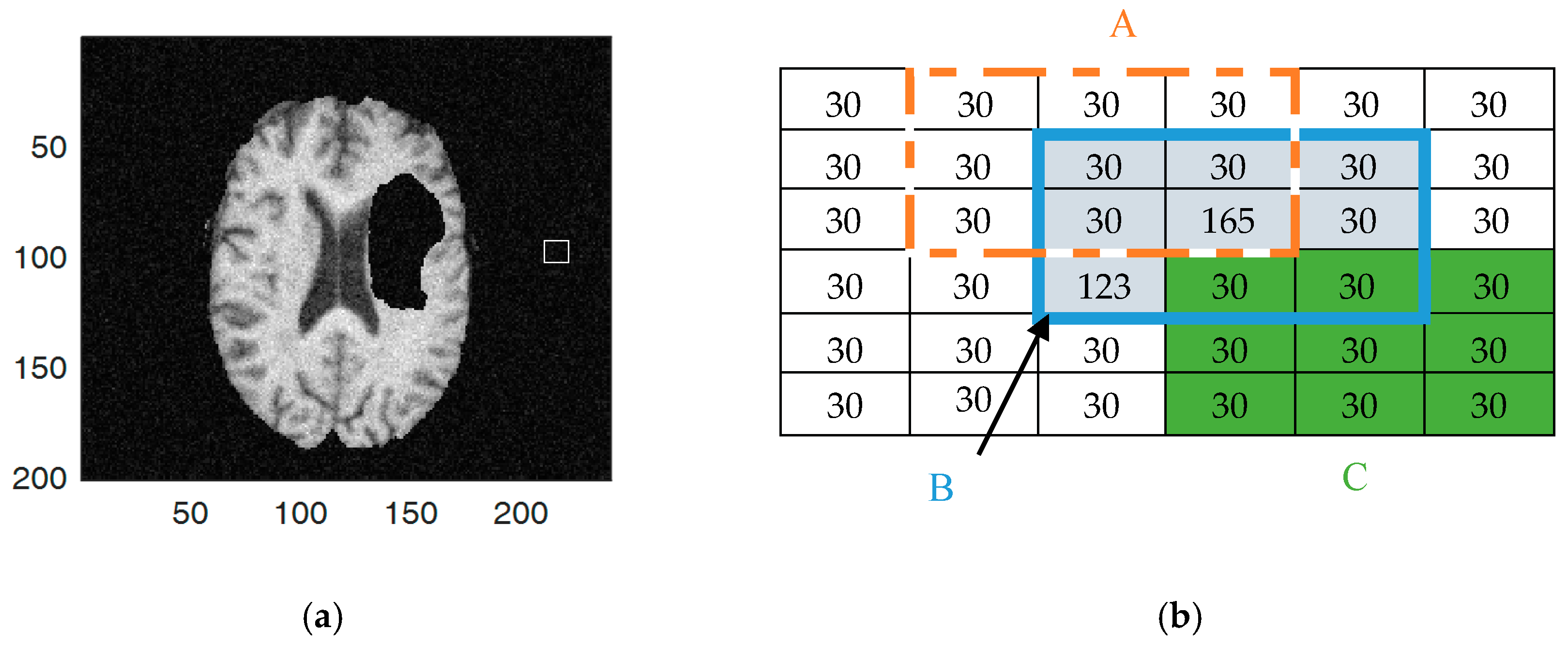
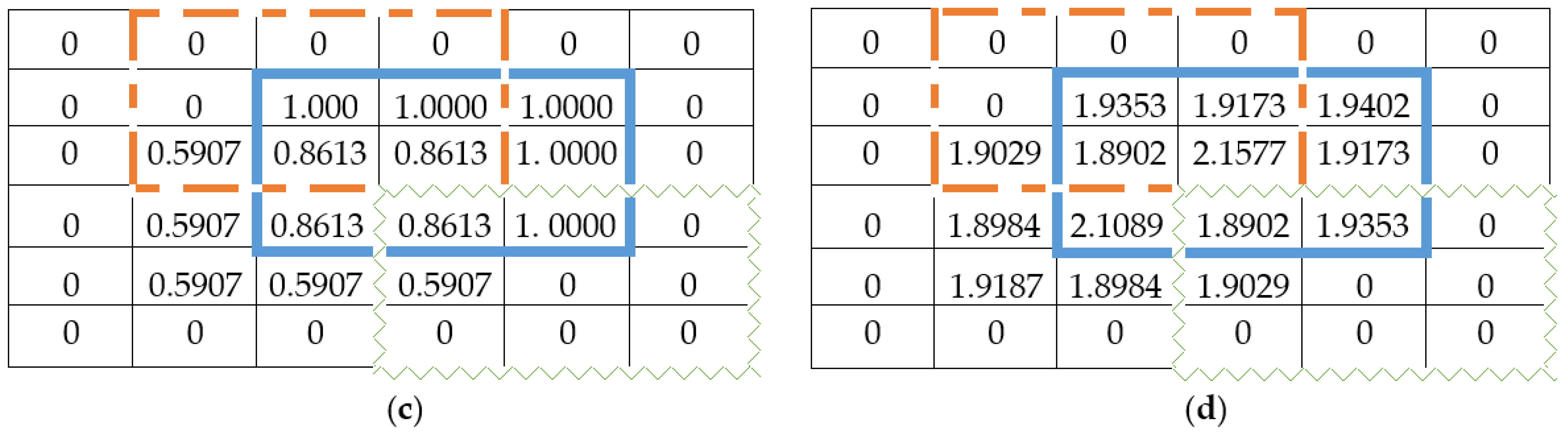
4.1. Local Intensity Variance

First, we improve the noise resistance by replacing the $\beta$ in Equation (7) with a weight that measuring local uniformity. Let $N_k$ be the neighborhood of a given size, e.g., $3\times 3$ pixels, around pixel $x_k$. The local intensity variance (LIV) of the pixel $x_k$ is defined as:

$$LI{V}_k=\frac{{\displaystyle {\sum }_{j\in N_k}{(x_j-\overline{x_k})}^2}}{\left|N_k\right|}$$

(8)

where $\left|N_k\right|$ denotes the number of pixels in $N_k$, and $\overline{x_k}$ is the mean grayscale taken over all pixels in $N_k$. LIV estimates the discrepancy of grayscales in the neighborhood normalized by the local average grayscale. A large LIV indicates higher level of noise within the neighborhood.

We then define a brightness weight for the pixel $x_k$ as:

$${\omega }_k=\frac{{\zeta }_k}{{\displaystyle {\sum }_{j\in N_k}{\zeta }_j}}$$

(9)

where:

$${\zeta }_k=\exp \left({\displaystyle \sum _{j\in N_k,k\ne j}LI{V}_j}\right)$$

(10)

Intuitively, ${\zeta }_k$ measures the noise level of neighborhood $N_k$ and ${\omega }_k$ is normalized over the neighborhood. Thus, a large ${\omega }_k$ indicates that pixel $x_k$ is brighter than its neighbors.

Finally, we define the variance for the pixel $x_k$ as:

$${\phi }_k=\{\begin{array}{l}2+{\omega }_k,\overline{x_k}<x_k\\ 2-{\omega }_k,\overline{x_k}>x_k\\ 0,\overline{x_k}=x_k\end{array}$$

(11)

The variance ${\phi }_k$ is larger for those pixels with high LIV (or brighter than its neighbors) and smaller otherwise. If the local average grayscale is equal to the grayscale of the central pixel, ${\phi }_k$ will be zero. The constant 2 in Equation (11) is determined through experiments and provides a balance between the convergence rate and the capability to preserve details.

We can now rewrite the objective function as follows:

$$J_{FCM}(U,V)={\displaystyle \sum _{i=1}^c{\displaystyle \sum _{k=1}^n{(u_{ik})}^m{\Vert x_k-v_i\Vert }^2}}+{\displaystyle \sum _{i=1}^c{\displaystyle \sum _{k=1}^n{\phi }_k{(u_{ik})}^m{\Vert \overline{x_k}-v_i\Vert }^2}}$$

(12)

Since ${\phi }_k$ is relevant only to the grayscales within a specified neighborhood, which is independent of any cluster, it only needs to be calculated once before the clustering process. This is very different from FCM_S, FLICM, and KWFLICM, where the contextual information must be updated for each pixel and each cluster in each iteration. Thus, Equation (12) will result in a much low computational cost.

The contextual information provided by ${\phi }_k$ is based on the heterogeneity of grayscale distribution within the neighborhood. This is different from existing methods that base the contextual information on the difference of the grayscales between neighboring pixels and cluster centroids. As a result, ${\phi }_k$ tends to produce a homogeneous clustering while local information used in existing methods [33] tend to generate clustering with more misclassified labels.

Figure 1a shows an image with Rician noise (Level 15), in which the white rectangle is an area of $6\times 6$ pixels. Figure 1b shows the greyscale value of pixels in this area, as well as three $3\times 3$ neighborhood areas A, B and C. Figure 1c,d show, respectively, the LIV and ${\phi }_k$ for each pixel.

4.2. Intuitionistic Fuzzy C-Means Clustering

We now change the fuzzy clusters from conventional fuzzy sets to intuitionistic fuzzy sets. According to the definition given in Section 2.1, we re-write the objective function in Equation (12) as follows:

$$J_{IFCM}(U,V)=\left({\displaystyle \sum _{i=1}^c{\displaystyle \sum _{k=1}^n{(u_{ik}^{\ast })}^m{\Vert x_k-v_i\Vert }^2}}+{\displaystyle \sum _{i=1}^c{\displaystyle \sum _{k=1}^n{\phi }_k{(u_{ik}^{\ast })}^m{\Vert \overline{x_k}-v_i\Vert }^2}}\right)+{\displaystyle \sum _{i=1}^c{\mathsf{\pi }}_i^{\ast }{e}^{1-{\mathsf{\pi }}_i^{\ast }}}$$

(13)

Here $u_{ik}^{\ast }=u_{ik}+{\mathsf{\pi }}_{ik}$ is the membership for pixel $x_k$ with respect to intuitionistic fuzzy cluster that has the centroid $v_i$, $u_{ik}$ is the membership degree, and ${\mathsf{\pi }}_{ik}$ is a hesitation degree.

The second term in the Equation (13) is called the intuitionistic fuzzy entropy (IFE) and measures the vagueness or ambiguity in the intuitionistic clusters. It is included to minimize the entropy of the histogram of the given data and therefore to maximize the number of good points in the cluster.

We can calculate the hesitation degrees using Yager’s definition [20]: $\nu (x)={(1-x^{\alpha })}^{1/\alpha }$, where $\alpha >0$, $\nu (1)=0$, and $\nu (0)=1$. Thus:

$${\mathsf{\pi }}_{ik}=1-u_{ik}-{\left(1-u_{ik}^{\alpha }\right)}^{1/\alpha }$$

(14)

and the variance ${\mathsf{\pi }}_i^{\ast }$ in the third term in Equation (13) is defined by:

$${\mathsf{\pi }}_i^{\ast }=\frac{1}{N}{\displaystyle \sum }_{k=1}^n{\mathsf{\pi }}_{ik}$$

(15)

Notice that the Yager class parameter $\alpha$ in Equation (14) controls the effect of local information and is crucial for the quality of the fuzzy clustering.

4.3. Kernel Intuitionistic FCM (KIFCM)

The Euclidean distance metric used in Equation (13) is valid under the assumption of uncorrelated cluster and cluster with the same spherical shape, that may be not true in real data. In addition, it is sensitive to perturbations and outliers. One way to address these problems is to use a different distance metrics, such as the Mahalanobis distance. Another way to deal with these problems is to use kernel functions to project the data into a higher dimensional space so that the data could be separated more easily [34]. An advantage of the latter method is that a so-called kernel trick can be used to transform linear algorithm into nonlinear one using dot product [35].

To improve segmentation accuracy and the robustness with respect to outliers, we utilize the kernel trick and replace the Euclidean distance ${\Vert x_k-v_i\Vert }^2$ with ${\Vert \Phi (x_k)-\Phi (v_i)\Vert }^2$. Accordingly, the objective function in Equation (13) can be re-written as:

$$J_{KIFCM}(U,V)=\left({\displaystyle \sum _{i=1}^c{\displaystyle \sum _{k=1}^n{(u_{ik}^{\ast })}^m{\Vert \Phi (\overline{x_k})-\Phi (v_i)\Vert }^2}}+{\displaystyle \sum _{i=1}^c{\displaystyle \sum _{k=1}^n{\phi }_k{(u_{ik})}^m{\Vert \Phi (\overline{x_k})-\Phi (v_i)\Vert }^2}}\right)+{\displaystyle \sum _{i=1}^c{\mathsf{\pi }}_i^{\ast }{e}^{1-{\mathsf{\pi }}_i^{\ast }}}$$

(16)

where $\Phi$ is an implicit nonlinear mapping and ${\Vert \Phi (x_k)-\Phi (v_i)\Vert }^2$ is the squared Euclidean distance between mapped pixels $\Phi (x_k)$ and $\Phi (v_i)$ in a feature space, which can be calculated using the kernel function in the input space as follows:

$${\Vert \Phi (x_k)-\Phi (v_i)\Vert }^2=K(x_k,x_k)+K(v_i,v_i)-2(x_k,v_i)$$

(17)

where $K()$ is a kernel function.

A widely-used kernel function is the Gaussian radial basis function (GRBF) [19]:

$$K(x_k,v_i)=\exp \left(\frac{-{\Vert x_k-v_i\Vert }^2}{{\sigma }^2}\right)$$

(18)

where the kernel parameter $\sigma$ determines the spread of the kernel and $\Vert x_k-v_i\Vert {}^2$ is the Euclidean distance between pixels in the original space. Using this kernel function, Equation (17) can be rewritten as:

$${\Vert \Phi (x_k)-\Phi (v_i)\Vert }^2=2\left(1-K(x_k,v_i)\right)$$

(19)

Substituting Equation (19) into Equation (16), we obtain our final objective function:

$$J_{KIFCM}(U,V)=2\left({\displaystyle \sum _{i=1}^c{\displaystyle \sum _{k=1}^n{(u_{ik}^{\ast })}^m(1-K(x_k,v_i)}})+{\displaystyle \sum _{i=1}^c{\displaystyle \sum _{k=1}^n{\phi }_k{(u_{ik})}^m\left(1-K(\overline{x_k},v_i)\right)}}\right)+{\displaystyle \sum _{i=1}^c{\mathsf{\pi }}_i^{\ast }{e}^{1-{\mathsf{\pi }}_i^{\ast }}}$$

(20)

Subject to the conditions required of $U$ and $V$ (see Section 2.2) and given parameters $m, \sigma$ and $\alpha$, Equation (20) will be minimized for membership degrees:

$$u_{ik}=\frac{{\left((1-K(x_k,v_i))+{\phi }_k(1-K(\overline{x_k},v_i))\right)}^{-1/(m-1)}}{{\displaystyle {\sum }_{j=1}^c{\left((1-K(x_k,v_j))+{\phi }_k(1-K(\overline{x_k},v_j))\right)}^{-1/(m-1)}}}$$

(21)

and centroids of intuitionistic fuzzy clusters:

$$v_i=\frac{{\displaystyle {\sum }_{k=1}^n{(u_{ik})}^m\times \left(K(x_k,v_i)x_k+{\phi }_{k}K(\overline{x_k},v_i)\overline{x_k}\right)}}{{\displaystyle {\sum }_{k=1}^n{(u_{ik})}^m\left(K(x_k,v_i)+{\phi }_{k}K(\overline{x_k},v_i)\right)}}$$

(22)

We call this formulation of the FCM clustering as the kernel-based Intuitionistic FCM (KIFCM) clustering.

5. The DNA Genetic Algorithm

In this section, we present a DNA genetic algorithm for the kernel-based intuitionistic fuzzy C-means clustering problem, which we call Algorithm2: KIFCM-DNAGA. This algorithm is a specialization of the generic DNA-GA presented in Section 2.3.

Depending on the calculation of ${\overline{x}}_i$ in Step 9, there can be variations of this algorithm. Specifically, if ${\overline{x}}_i$ is the average greyscale, we call this algorithm KIFCM1-DNAGA and if ${\overline{x}}_i$ is the median greyscale the algorithm is denoted as KIFCM2-DNAGA. We will discuss more details in the following subsections.

KIFCM-DNAGA contains three nested loops. The outer most loop iterates the evolution process, and is typically controlled by a user-specified constant, such as the number of iterations. Each of the inner loops is repeated for each of the $n$ pixels. In the inner most loop, each pixel needs to be compared to the centroids of the $c$ fuzzy clusters and the distance calculations involve the $d$ dimensions. Thus, the complexity of this algorithm is $O(c{n}^{2}d)$. Notice that the kernel matrix is computed only once at the very beginning of the program.

The detailed description of KIFCM-DANGA is presented in Algorithm 2 below.

Algorithm 2: KIFCM-DNAGA

Input: $ϵ$: convergence threshold   $t$: maximum number of iterations   $c$: the number of fuzzy clusters    $K$: a kernel function   $M$: an MRI image   $N$: the size of the population Output: $U$: the membership matrix       $V$: the centroids of fuzzy clusters Method: POP = create $N$ randomly generated individuals encoded as DNA strings $t=0$; Initialize $U^{\left(0\right)}$ and $V$ While $t=0$ or $\Vert U^t-U^{t-1}\Vert >ϵ$ do  $t=t+1$  for $p\in POP$ do   decode $m$, $\alpha$, and $\sigma$   for every pixel $x_k\in M$    Calculate ${\phi }_k$ using Equation (11)    Calculate ${\overline{x}}_i$    Calculate $u_{ik}$ and $v_i$ using Equations (21) and (22), respectively   Calculate fitness value for $p$ using Equation (20)  V = V of the best fit individual in POP  NewPOP = apply selection op on POP  NewPOP = NewPOP ${\displaystyle \cup }$ apply DNA genetic operations on POP  POP = apply reconstruction op NewPOP  Return $U^t$ and $V$

5.1. DNA Encoding and Decoding

Recall that if values of the model parameters $m, \sigma$ and $\alpha$ are given, Equations (21) and (22) can be used to calculate the fitness value, and the clustering (i.e., the membership degrees and cluster centroids). The optimal clustering is obtained provided the optimal values for these parameters are given. As pointed out by Chaira [12] , the values of parameters $m$ and $\alpha$ will affect the performance of IFCM, and by Graves and Pedrycz [36], the value of parameter $\sigma$ in a kernel function will affect the performance. Our algorithm is designed to find the optimal values for parameters $m, \sigma$ and $\alpha$, and to obtain the optimal clustering along the way.

In this algorithm, an individual, a potential solution, consists of values for three variables $v_1$ representing parameter $\sigma$, $v_2$ representing $\alpha$, and $v_3$ representing $m$. We encode each variable as a string of $n$ base-4 digits, where n is a system parameter and each digit represents a nucleotide bases, for example, 0 for A, 1 for G, 2 for C, and 3 for T. Figure 2 shows an example of an encoded individual, where n = 6.

For decoding, each variable $v_i$ is mapped into a decimal number as follows:

$$c{v}_i={\displaystyle \sum }_{j=1}^{n}bit\left(j\right)\times 4^{j-1}$$

(23)

where $bit(j)$ is the j-th digit from the left of the current encoding segment for $v_i$. Depending on the bounds of the variable, the value of the variable is obtained as follows:

$$v_i=\frac{c{v}_i}{4^n-1}\left(h_i-l_i\right)+l_i$$

(24)

where $l_i$ and $h_i$ are the lowest and the highest values of the variable $v_i$, and $\left(h_i-l_i\right)/4^n-1$ is the precision of the decoded value for $v_i$.

For example, in Figure 2 the encoding of $\alpha \left(\mathrm{i}.\mathrm{e}.,v_2\right)$ is the base-4 number 120132, representing GCAGTC. The corresponding decimal number is $c{v}_2=1566$. If the range of $\alpha$ is $\left[1, 15\right]$, the decoded value of $\alpha$ is 6.35.

5.2. The Initialization

In Step 1, $N$ individuals encoded as described in the previous subsection are randomly generated to form the initial population. For each nucleotide base in an individual’s DNA strand, we randomly assign one of A, C, G, and T (in fact, the base-4 digit corresponding to these amino acids). Unlike existing DNA-GAs which assign A, C, G, T with an equal probability 0.25, our algorithm assigns A, C, G, T with differential probabilities 0.156, 0.343, 0.344, and 0.157, respectively. These probabilities are chosen according to the nature of biological structures [37].

5.3. Selection Operator

In Step 14, a 50% of the current population is selected to participate in genetic operations that generate new individuals in the next generation. In general, three types of selection methods, namely roulette wheel, ranking and tournament have been used in various DNA-GAs. To be specific, we describe the tournament selection here. In this method, pairs of individuals from the current population are randomly selected and for each pair, the individual with the higher fitness value is selected. In addition, the so-called elitism strategy is also applied, which will include the best fit individual among the selected individuals.

5.4. DNA Genetic Operators

In Step 15, different types of genetic operations are applied randomly to randomly selected individuals in the new population. These operations are applied in sequence to evolve the new generation. The operations are discussed in the following subsections. Each of these operations will generate offspring individuals from parent individuals and preserve the size of the generation. After an operator is applied to the parent individuals, the offspring individuals survive and participate in the next operation.

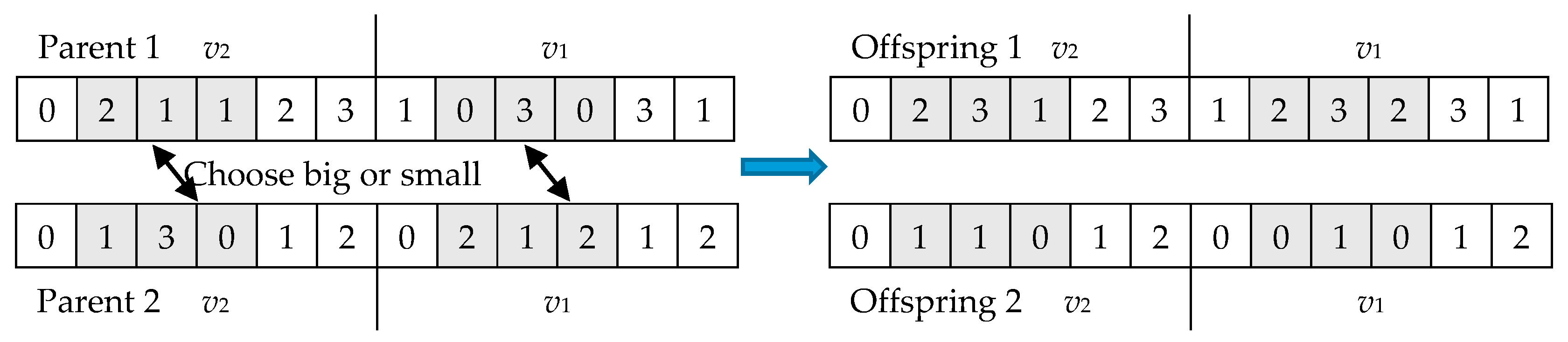
5.4.1. Crossover Operator

A crossover operator generates two offspring individuals from two randomly selected parent individuals by swapping and mixing nucleotide bases of randomly selected DNA segments of the two parents.

Figure 3 shows an example illustrating the crossover operator. To ease the presentation. Only two variables are shown for individuals and each variable has a sequence of 6 nucleotide bases. Assume that the shaded segments in the two parents are randomly selected. To generate the two offspring individuals, the corresponding nucleotide bases are swapped according to the “choose big” and “choose small” strategies [38]. Namely, the offspring 1 is created by choosing in each nucleotide bases the larger values between the two parents and the offspring 2 the smaller values. Consider the shaded segment in $v_2$ in the two parents. The sequences are 211 and 130. The larger digits for each position in these two sequences are respectively 2, 3, and 1. Similarly, the smaller digits are 1, 1, and 0. Thus, in this segment, offspring 1 has the sequence 231 and offspring 2 has the sequence 110.

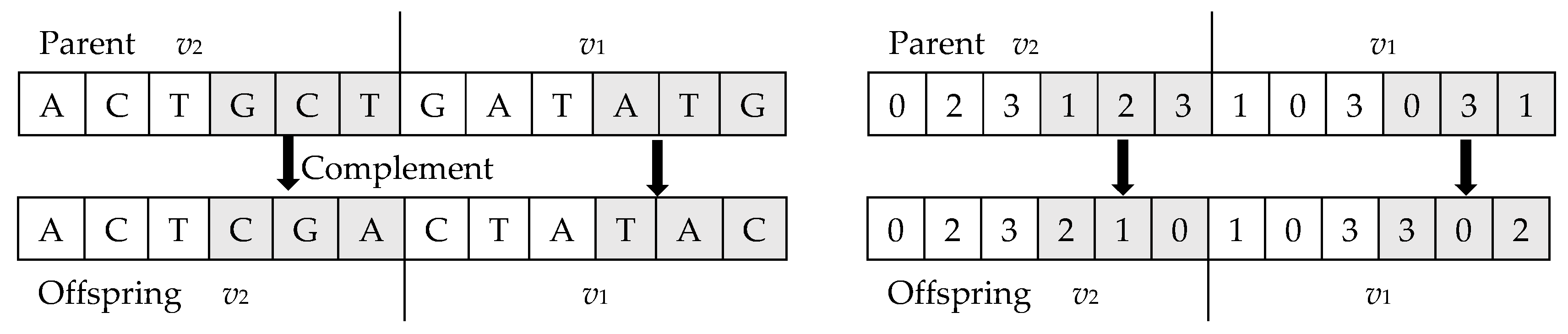
5.4.2. Mutation Operator

A mutation operator generates an offspring from a parent by randomly changing (mutating) the digit at a randomly selected nucleotide base.

Unlike existing GAs which select position to mutate with an equal probability, we adapt a strategy of a shifting probability. Specifically, we divide the DNA strand of an individual into a high bit section and a low bit section, and mutate digits in different sections using the following probabilities: $P_{mh}$ for high bit section and $P_{ml}$ for low bit section:

$$\{\begin{array}{l}{P}_{mh}=a_1+\frac{b_1}{1+\exp [c(g-g_0)]}\\ P_{ml}=a_1+\frac{b_1}{1+\exp [-c(g-g_0)]}\end{array}$$

(25)

where $a_1$ is the initial mutation probability, $b_1$ is the range of mutation probability, $g$ is the evolution generation, $g_0$ is the generation where a greater mutation probability occurs and $c$ is the speed of change.

The idea is inspired by the DNA “hot spots” and “cold spots” in biology [39]. Nucleotide bases in “cold spots” mutate more slowly than those in “hot spots”. To mimic this phenomenon, $P_{mh}$ and $P_{ml}$ are designed to change with the evolution stage. At the beginning of the evolution $P_{mh}$ will be larger than $P_{ml}$. As the evolution progresses, $P_{mh}$ will be gradually reduced and $P_{ml}$ increased.

5.4.3. Reconstruction Operator

In Step 16, the reconstruction operator is applied to every individual in the new population with a probability $P_r$. The reconstruction operator generates an offspring by replacing each nucleotide base in a randomly selected segment of each variable by the complementary nucleotide base, namely A and T replace each other and so do G and C. This operation is inspired by the DNA double helix complementary principle [40].

Figure 4 shows an example of the reconstruction operator. On the left, the nucleotide symbols are shown in the parent and the offspring and on the right the encoded base-4 numbers are shown for the same parent and offspring. Assume that the right-most 3 bits of each variable are randomly chosen to perform the operation based on Waston-Crick [41] pairs. The nucleotide bases ATG (encoded in 031) in $v_1$, and GCT (encoded in 123) with $v_2$ in a parent are changed to TAC (encoded in 302) and CGA (encoded in 210), respectively, in the offspring.

After the complementary operation is applied to the new generation, new random individuals will be generated as needed to keep the population size at $N$.

6. Experiments and Results

In this section, we present results from our experiments.

6.1. Experiment Setup

We compared our algorithm with six state-of-the-art soft clustering algorithms, including GKFCM1 [21], GKFCM2 [21], FLICM [2], KWFLICM [33], MICO [6], and RSCFCM [5].

These algorithms are compared using three types of data: a set of UCI machine learning datasets [42], a set of synthetic MRI data, and a set of clinical MRI data. The UCI datasets include Haberman’s Survival Data, Contraceptive Method Choice, Wisconsin Prognostic Breast Cancer, and SPECT Heart Data, with details are shown in

Table 1. The detailed features of UCI datasets.

Datasets	Number of Instances	Number of Attributes	Number of Classification
Haberman’s Surviva1 Data	306	3	2
Contraceptive Method Choice	1473	9	3
Wisconsin Prognostic Breast Cancer	198	34	2
SPECT Heart Data	267	22	2

.

The synthetic brain MR images includes a T1-weighted axial slice with 217 × 181 pixels corrupted with 7% noise and 20% grayscale, a T1-weighted sagittal slice with 181 × 217 pixels corrupted with 7% noise and 20% grayscale, and a T1-weighted axial slice with 217 × 181 pixels corrupted with 10% Rician noise.

The clinical brain MR images include two collections of datasets. The first collection is the dataset used by MICCAI BRATS 2014 challenge [1]. This dataset contains 220 clinical samples and each sample has a sequence of 155 T1-weighted axial slice images of 240 × 240 pixels. We randomly selected three samples (whose files are pat266_1, pat192_1, and pat013_1) and among the 155 slice images of each selected sample, we selected one slice that contains the most details and features and has the best visual quality (specifically, the 80-th, 86-th, and 90-th slice from the three samples, respectively). The second collection is the MR images collected using a Philips Medical Systems Intera 3T instrument obtained from the brain development project [43]. This collection contains 581 samples, and for each sample from 150 to 200 slices. We also randomly selected a sample (the 160-th sample) and a coronal slice (the 80th slice), which is of 512 × 300 pixels.

We measure the performance of the clustering algorithms using three metrics: the Jaccard Similarity (JS) [44], adjusted mutual information (AMI) and adjusted rand index (ARI) [45].

• The Jaccard Similarity is defined by:

  $$JS(S_1,S_2)=\frac{|S_1\cap S_2|}{|S_1\cup S_2|}$$

  (26)

  where S₁ is the segmented volume and S₂ is the ground truth volume.
• AMI is defined as follows:

  $$AMI=\frac{MI-E(MI)}{\sqrt{H(S_1)\cdot H(S_2)}-E(MI)}$$

  (27)

  where $H(S_1)$, $H(S_2)$ are the entropies for $S_1$ and $S_2$, respectively. Mutual information MI quantifies the value of information shared between the two random variables and can be defined using the entropy definitions. $E(MI)={\displaystyle {{\displaystyle \sum }}_{\Gamma }MI(\Gamma })P(\Gamma )$.
• ARI is defined as follows:

  $$ARI=\frac{2(N_{00}{N}_{11}-N_{01}{N}_{10})}{(N_{00}+N_{01})(N_{01}+N_{11})+(N_{00}+N_{10})(N_{10}+N_{11})}$$

  (28)

  where N₁₁ denotes the number of pairs that are in the same cluster in both U and V, N₀₀ denotes the number of pairs that are in different clusters in both U and V, N₀₁ denotes the number of pairs that are in the same cluster in U but in different clusters in V, and N₁₀ denotes the number of pairs that are in different clusters in U but in the same cluster in V.

These metrics are commonly used to compare the performance of clustering algorithms. For all three matrices, a higher value indicates a better clustering result, with the highest value being 1.

We implemented the algorithms in MATLAB. The experiments were conducted using neighborhood of 3 × 3 pixels. The termination conditions include a maximum number of iterations 𝑡 = 100 and convergence threshold 𝜀 = 0.001.

6.2. Results on UCI Datasets

In this experiment, we investigate how our algorithm performs for generic FCM clustering by using the set of UCI machine learning datasets (see Table 1). The same UCI datasets are commonly used in machine learning research [36]. Because these are not image data, we set the brightness variance ${\phi }_k$ to 0 in these experiments.

As shown in

Table 2. Clustering results for UCI machine learning datasets.

Title	Method	Parameters	AMI	ARI
Haberman’s Surviva1 Data	GKFCM1	$c=2,m=2,\sigma =0.5$	0.7263	0.6430
	GKFCM2	$c=2,m=2,\sigma =0.5$	0.7221	0.6332
	FLICM	$c=2,m=2$	0.9509	0.8620
	KWFLICM	$c=2,m=2,\sigma =0.5$	0.9386	0.8497
	MICO	$c=2,m=2$	0.7319	0.6430
	RSCFCM	$c=2,m=2.5$	0.9406	0.8587
	KIFCM1-DNAGA	$c=2,m=2.06,\alpha =11.03,\sigma =50.03$	0.9704	0.8815
Contraceptive Method Choice	GKFCM1	$c=3,m=2,\sigma =1.1$	0.6534	0.6544
	GKFCM2	$c=3,m=2,\sigma =1.1$	0.6525	0.6525
	FLICM	$c=3,m=2$	0.7366	0.7366
	KWFLICM	$c=3,m=1.7,\sigma =1.1$	0.7577	0.7577
	MICO	$c=3,m=2$	0.6477	0.6477
	RSCFCM	$c=3,m=2$	0.6853	0.7515
	KIFCM1-DNAGA	$c=3,m=2.45,\alpha =3.25,\sigma =2.12$	0.7991	0.8021
Wisconsin Prognostic Breast Cancer	GKFCM1	$c=2,m=2,\sigma =150$	0.9708	0.9687
	GKFCM2	$c=2,m=2,\sigma =150$	0.9665	0.9644
	FLICM	$c=2,m=2$	0.9451	0.9430
	KWFLICM	$c=2,m=2,\sigma =150$	0.9771	0.9750
	MICO	$c=2,m=2$	0.9808	0.9787
	RSCFCM	$c=2,m=2$	0.9832	0.9815
	KIFCM1-DNAGA	$c=2,m=3.13,\alpha =1.50,\sigma =154.84$	0.9865	0.9844
SPECT Heart Data	GKFCM1	$c=2,m=2,\sigma =150$	0.6365	0.7039
	GKFCM2	$c=2,m=2,\sigma =150$	0.7264	0.7264
	FLICM	$c=2,m=2$	0.8350	0.8350
	KWFLICM	$c=2,m=2,\sigma =150$	0.8915	0.8915
	MICO	$c=2,m=2$	0.7339	0.7339
	RSCFCM	$c=2,m=2$	0.8488	0.8500
	KIFCM1-DNAGA	$c=2,m=3.42,\alpha =6.04,\sigma =156.2$	0.9174	0.9213

, KIFCM1-DNAGA can obtain a higher AMI and ARI than other algorithms, especially for datasets of a higher complexity. Moreover, algorithms using kernel functions show a better performance than those traditional algorithms, such as MICO, RSCFCM. The optimized results are marked in bold.

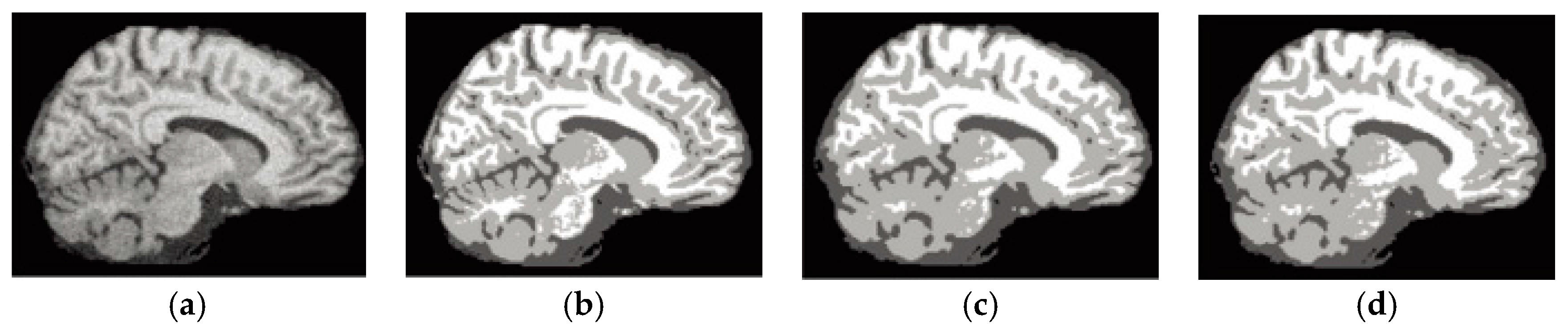
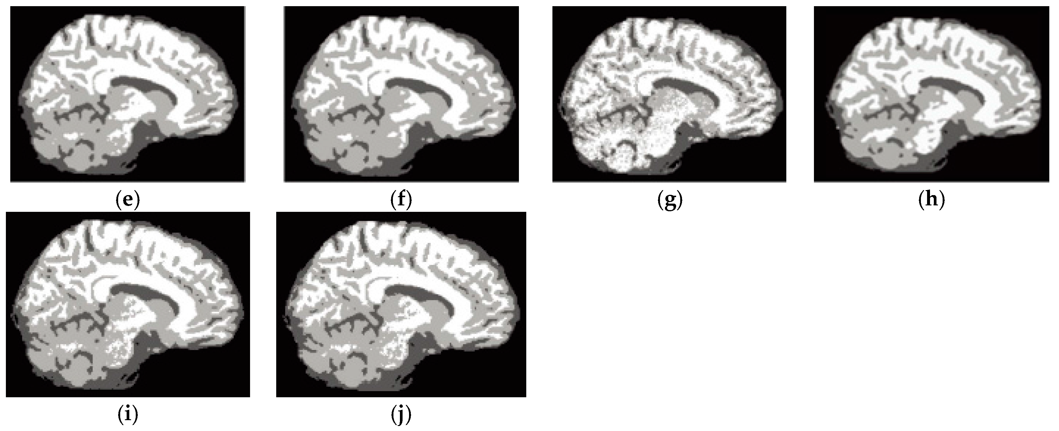
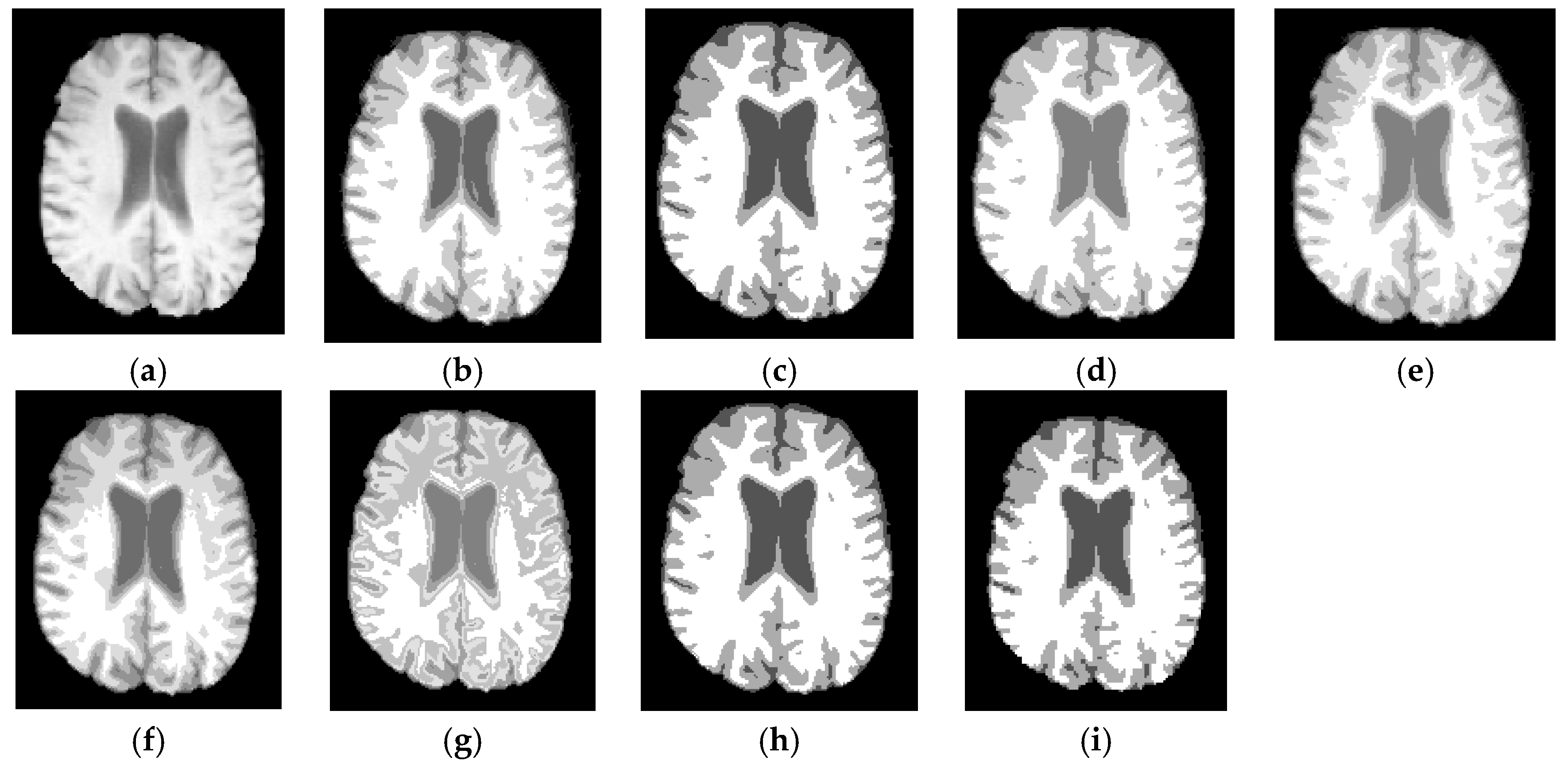
6.3. Results on Synthetic Brain MR Images

We performed several experiments using the Simulated Brain Database (SBD) [46], which contains a set of realistic MR volumes produced by an MR imaging simulator. These data come with the ground truth, i.e., pixels are labeled for CSF, GM, and WM regions.

The first experiment is to segment a T1-weighted axial slice with 217 × 181 pixels corrupted with 7% noise and 20% grayscale non-uniformity into WM, GM, and CSF. Figure 5 shows the segmentation results and

Table 3. JS and running time on the T1-weighted axial slice from SBD with 7% noise and 20% grayscale non-uniformity.

Algorithm	GKFCM1	GKFCM2	FLICM	KW FLICM	MICO	RSCFCM	KIFCM1-DNAGA	KIFCM2-DNAGA
WM	0.930	0.933	0.941	0.937	0.894	0.898	0.940	0.941
GM	0.822	0.855	0.860	0.852	0.782	0.842	0.864	0.868
CSF	0.781	0.847	0.829	0.805	0.860	0.882	0.863	0.867
Average	0.844	0.879	0.876	0.865	0.845	0.874	0.889	0.892
Time (s)	0.911	0.586	3.403	139.470	0.673	2.530	0.356	0.282

summarizes the JS and average running times.

According to Table 3, KIFCM1-DNAGA and KIFCM2-DNAGA outperform the other 6 algorithms. On average, the improvement on JS is about 1.3–4.8%. The best results are marked in bold.

The second experiment is to segment a T1-weighted sagittal slice with 181 × 217 pixels corrupted with 7% noise and 20% grayscale non-uniformity. This image is chosen to show the capability of preserving details. The segmentation results are shown in Figure 6 and JS are presented in

Table 4. JS and running time on the T1-weighted sagittal slice from SBD with 7% noise and 20% grayscale non-uniformity.

Algorithm	GKFCM1	GKFCM2	FLICM	KWFLICM	MICO	RSCFCM	KIFCM1-DNAGA	KIFCM2-DNAGA
WM	0.773	0.775	0.771	0.765	0.672	0.702	0.785	0.788
GM	0.796	0.806	0.794	0.791	0.669	0.743	0.815	0.816
CSF	0.834	0.852	0.835	0.824	0.869	0.813	0.871	0.872
Average	0.801	0.811	0.800	0.794	0.736	0.753	0.824	0.825
Time (s)	1.377	1.797	5.392	166.717	0.751	0.786	0.348	0.329

.

Based on Table 4, the average JSs of KIFCM1-DNAGA and KIFCM2-DNAGA are better than the other algorithms by about 1.4–8.9%. The best results are marked in bold.

The third experiment is to segment a T1-weighted axial slice (number 91) with 217 × 181 pixels corrupted with 10% Rician noise. The Rician noise commonly affects MR images [47]. The segmentation results are shown in Figure 7 and the JS with average running times is given in

Table 5. JS and running time on the T1-weighted axial slice (number 91) from SBD corrupted with 10% Rician noise.

Algorithm	GKFCM1	GKFCM2	FLICM	KWFLICM	MICO	RSCFCM	KIFCM1-DNAGA	KIFCM2-DNAGA
WM	0.931	0.921	0.929	0.927	0.885	0.891	0.926	0.925
GM	0.804	0.827	0.831	0.821	0.777	0.803	0.838	0.840
CSF	0.826	0.872	0.861	0.846	0.889	0.876	0.887	0.892
Average	0.854	0.873	0.874	0.865	0.850	0.857	0.884	0.886
Time (s)	1.836	1.869	2.953	124.922	0.649	0.781	0.218	0.220

. The best results are marked in bold.

Again, the average JSs of KIFCM1-DNAGA and KIFCM2-DNAGA are better than the other algorithms (by about 1.20 to 3.6%). The higher JSs implies that our algorithms do a better job in preserving image details in the presence of noise and grayscale homogeneity. The best results are marked in bold.

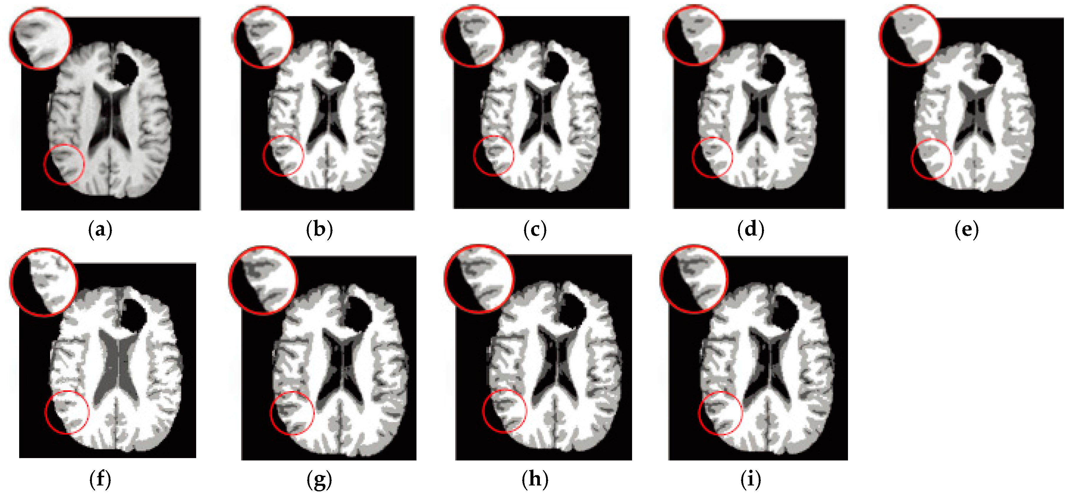
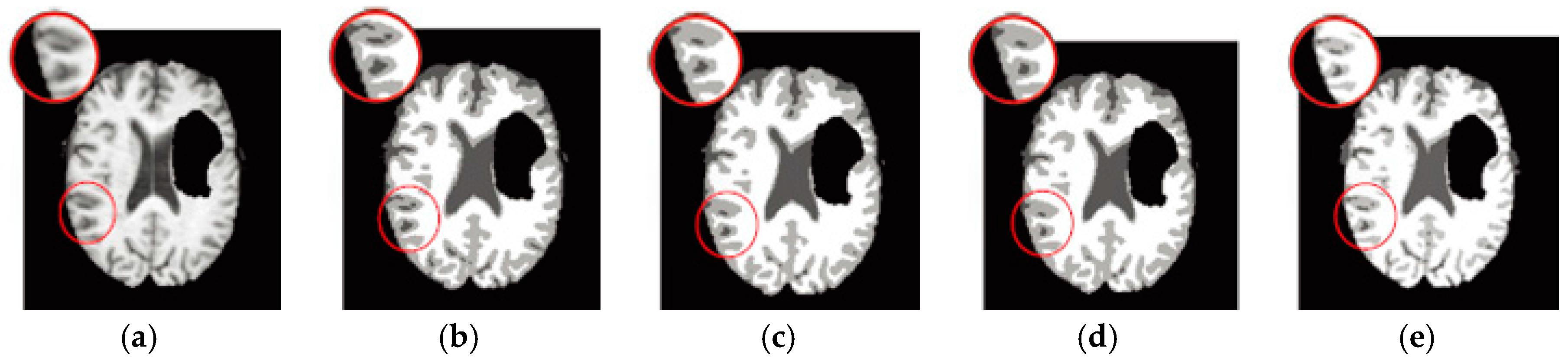
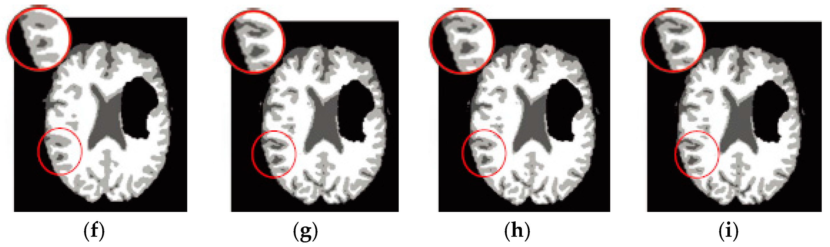
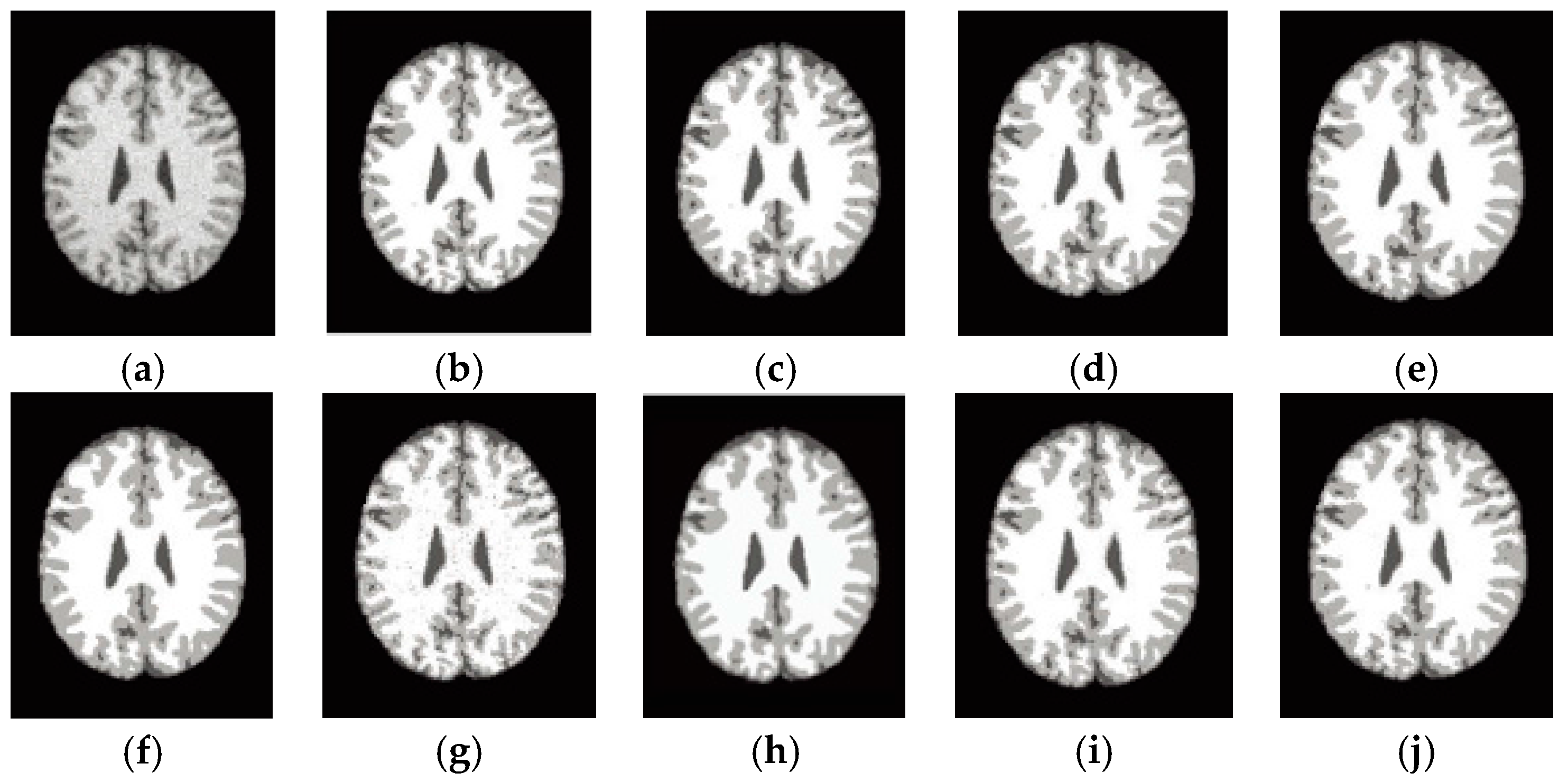
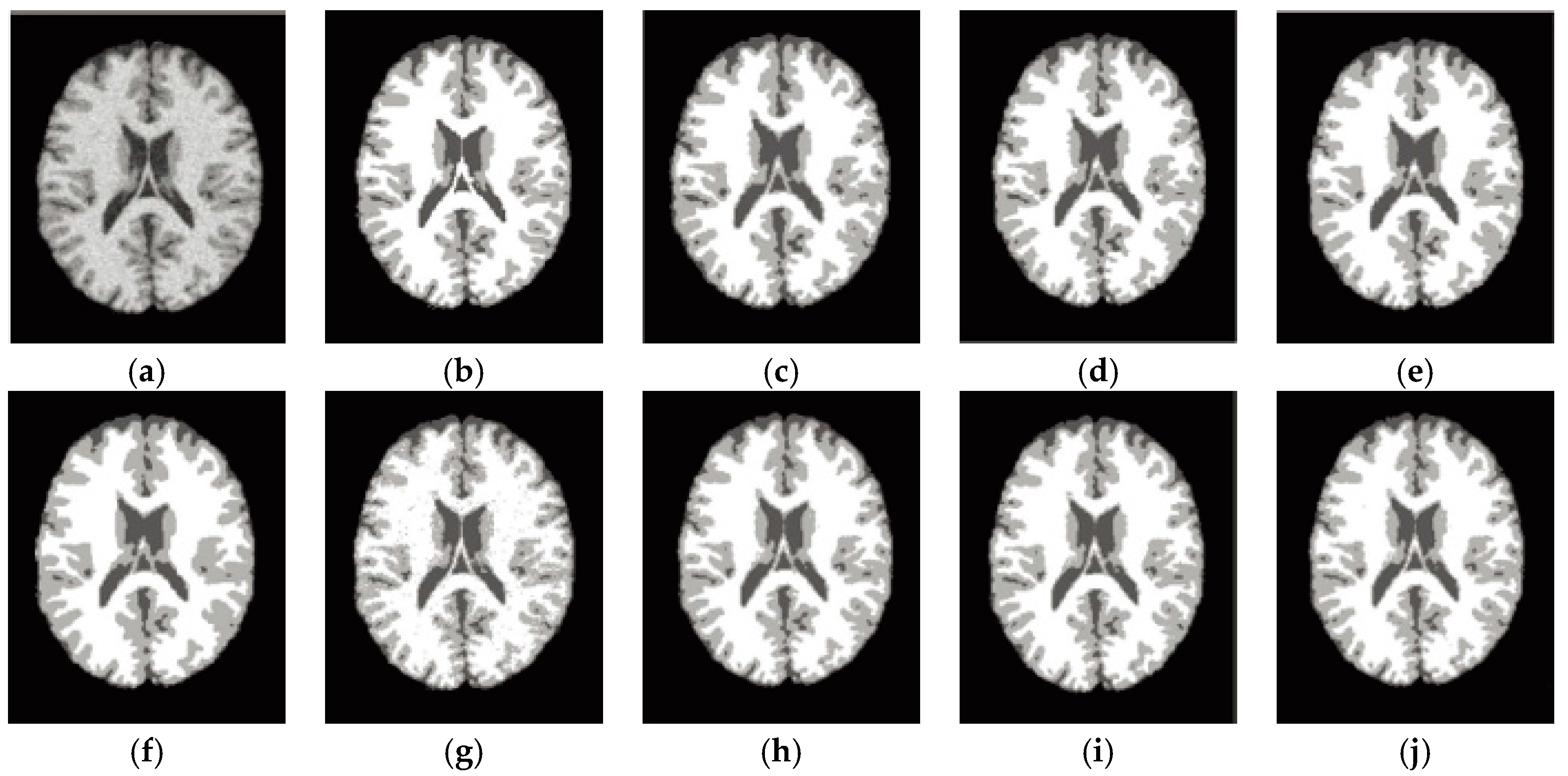
6.4. Results on Clinical Brain MR Images

In these experiments, we used MR images from two collections of clinical MRI datasets. We first used three T1-weighted axial slices (slice rank 80, 86, and 90, denoted as Brats1, Brats2, and Brats3, respectively) of 240 × 240 pixels included in MICCAI BRATS 2014 challenge. In these images, pixels with grayscale from black to white represent respectively, the background, CSF, GM, and WM. It is worth noting that clustering is carried out only for CSF, GM, and WM, with the pathology region being treated as the background. We then used a coronal slice (denoted as Brats4) with 512 × 300 pixels [43].

Figure 8 shows the results for Brats1 and Figure 9 shows the results for Brats2. The area within the red circles are enlarged to show more details. Figure 10 and Figure 11 show the results for Brats3 and Brats4.

Since the images come only with the ground truth for the pathology and do not have the ground truth for normal tissues, we also used the entropy-based metric [48] to measure the quality of the algorithms. This metric aims to maximize the uniformity of pixels within each segmented region and to minimize the uniformity across the regions. The entropy of an image region 𝑗 is defined as:

$$H(R_j)=-{\displaystyle \sum _{m\in V_j}\frac{L_j(m)}{S_j}}\log \frac{L_j(m)}{S_j}$$

(29)

where $V_j$ is the set of all possible grayscales in region $j$, $L_j(m)$ is the number of pixels belonging to region $j$ with grayscale $m$, and $S_j$ is the area of region $j$. For a grayscale image $j$, the 𝐸 measure is defined as:

$$E={\displaystyle \sum _{j=1}^c\left(\frac{S_j}{S_t}\right)}H(R_j)+\left(-{\displaystyle \sum _{j=1}^c\left(\frac{S_j}{S_t}\right)\log \frac{S_j}{S_t}}\right)$$

(30)

where the first term represents the expected region entropy of the segmentation and the second term is the layout entropy. Notice that smaller 𝐸 indicates a better segmentation.

Table 6. Segmentation performance in 𝐸 measure and running times on the Brats1, Brats2, Brats3 and Brats4.

Image	Measure	GKFCM1	GKFCM2	FLICM	KWFLICM	MICO	RSCFCM	KIFCM1-DNAGA	KIFCM2-DNAGA
Brats1	E	1.311	1.288	1.392	1.424	1.309	1.314	1.274	1.270
	Time (s)	2.591	1.516	9.510	6.354	1.747	12.622	1.185	1.111
Brats2	E	1.307	1.297	1.336	1.340	1.298	1.307	1.273	1.271
	Time (s)	1.576	1.115	5.170	4.002	1.546	1.674	1.091	0.827
Brats3	E	1.295	1.285	1.324	1.328	1.286	1.295	1.261	1.259
	Time (s)	1.564	1.103	5.158	4.002	1.534	1.662	1.079	0.815
Brats4	E	1.425	1.415	1.454	1.458	1.416	1.424	1.391	1.389
	Time (s)	6.099	4.301	20.116	15.611	5.982	6.481	4.2081	3.1785

shows the segmentation accuracy in terms of the $E$ measure as well as the running times of the algorithms. The 𝐸 values are calculated only for WM, GM, and CSF regions. The best results are marked in bold.

From Table 6, our algorithms achieve smaller 𝐸 than other algorithms. Visually, GKFCM1 (Subfigure b in Figure 8, Figure 9, Figure 10 and Figure 11) and GKFCM2 (Subfigure c in Figure 8, Figure 9, Figure 10 and Figure 11) achieve good results but they are unable to preserve fine details. For example, CSF was incorrectly broken, possibly due to the difficulty in estimating parameter η_j. On the other hand, FLICM (Subfigure d in Figure 8, Figure 9, Figure 10 and Figure 11) and KWFLICM (Subfigure e in Figure 8, Figure 9, Figure 10 and Figure 11) yield smooth areas but they do not preserve fine details. For example, CSF in those results is smaller than the surrounding GM and WM. This may be because the difficulty to estimate optimal values for parameters G_ij and $G_{ij}^{\prime }$. For MICO algorithm (Subfigure f in Figure 8, Figure 9, Figure 10 and Figure 11), the edges are not smooth enough, hence the CSF is not well preserved. For RSCFCM algorithm (Subfigure g in Figure 8, Figure 9, Figure 10 and Figure 11), many details are missing. In comparison, KIFCM1-DNAGA (Subfigure h in Figure 8, Figure 9, Figure 10 and Figure 11) and KIFCM2-DNAGA (Subfigure i in Figure 8, Figure 9, Figure 10 and Figure 11) show good balance between smooth borders and image details. It achieves better balance in preserving image details in presence of different noise than the 6 other algorithms. Especially, even with a larger MR image, the proposed approach still performs well on E and running time measure.

7. Discussion

In this section, we discuss and compare the computational complexity and running times of ours and the other algorithms used in our experiments.

Table 7. Computational complexity.

Algorithm	GKFCM1	GKFCM2	FLICM	KWFLICM	MICO	RSCFCM	KIFCM1-DNAGA	KIFCM2-DNAGA
Overall complexity	$O(cn{d}^2)$	$O(cn{d}^2)$	$O(cnd)$	$O(cnd)$	$O(c{n}^{2}d)$	$O(cnd)$	$O(c{n}^{2}d)$	$O(c{n}^{2}d)$

shows a summary of the computational complexity of the eight algorithms. Assuming all algorithms go through exactly the same number of rounds of evolution, the complexity of these algorithms differs mainly in the number of times each pixel is processed within a single round of evolution.

The GKFCM requires $O(cn{d}^2)$ to compute the partition matrix in each iteration [36]. If the kernel matrix is computed at the beginning of each iteration, the complexity of the partition matrix is $O(cnd)$. Each of the FLICM, MICO, and RSCFCM requires $O(cnd)$ for each iteration, in which the kernel matrix requires the kernel function be evaluated $cn$ times. The complexity for the kernel algorithms depends on the kernel used. The complexity given in Table 7 is for the Gaussian radial basis function. It is also assumed that the kernel matrix is computed once rather than at every iteration for the KIFCM-DNAGA algorithm.

To compare the efficiency of the algorithms, we measured the running time (in seconds) averaged over 10 runs for Brain MR images experiments mentioned in Section 6. For each run, the initial population is made identical for all algorithms. Figure 12 shows the results.

As shown in Figure 12, GKFCM1 and GKFCM2 have the longest running time. This is perhaps due to the parameter η_j used by the algorithms, which needs an additional loop over all clusters to update the local contextual information. MICO comes next with running times span 1.3 to 2.85 s. It performs fast calculations owing to the convexity of its energy function particularly in the presence of less noise, but tends to have many iterations in the presence of high level noise. RSCFCM spent about 1.05 to 2.95 s for the experiments. It uses a spatial fuzzy factor that is constructed based on the posterior and prior probabilities and takes the spatial direction into account. That is likely to increase the computational cost. FLICM and KWFLICM have similar performance. FICM uses parameter G_ij, which needs an additional loop over the neighborhood of the current pixel to calculate the local information in every iteration, and KWFLICM used parameter $G_{ij}^{\prime }$, which requires two additional loops to process the neighborhood. Finally, KIFCM1-DNAGA and KIFCM2-DNAGA both incorporate local contextual information obtained by LVC, which only needs to be calculated once. As a result, both algorithms require about 0.25–1.55 s to run the experiments, which is the lowest among the algorithms.

8. Conclusions

In this paper, we introduce a new formulation of the MRI segmentation problem as a kernel-based intuitionistic fuzzy C-means (KIFCM) clustering problem and proposed a new DNA-based genetic algorithm to learn the optimal KIFCM clustering. While this algorithm searches the solution space for the optimal model parameters, it also obtains the optimal clustering, therefore the optimal MRI segmentation. We perform empirical study by comparing our method with six state-of-the-art soft clustering methods using a set of UCI data mining data sets and a set of synthetic and clinic MRI data. Our preliminary results show that our method outperforms other methods in both the clustering metrics (against the ground truth) and the computational efficiency. For the future work, we plan to further improve the KIFCM-DNAGA and test it on a larger set of clinical MRIs.

References

1. Elazab, A.; AbdulAzeem, Y.M.; Wu, S.; Hu, Q. Robust kernelized local information fuzzy C-means clustering for brain magnetic resonance image segmentation. J. X-ray Sci. Technol. 2016, 24, 489–507. [Google Scholar] [CrossRef] [PubMed]
2. Krinidis, S.; Chatzis, V. A Robust Fuzzy Local Information C-Means Clustering Algorithm. IEEE Trans. Image Process. 2010, 19, 1328–1337. [Google Scholar] [CrossRef] [PubMed]
3. Nikou, C.; Galatsanos, N.P.; Likas, A.C. A class-adaptive spatially variant mixture model for image segmentation. IEEE Trans. Image Process. 2007, 16, 1121–1130. [Google Scholar] [CrossRef] [PubMed]
4. Cai, W.L.; Chen, S.C.; Zhang, D.Q. Fast and robust fuzzy c-means clustering algorithms incorporating local information for image segmentation. Pattern Recogn. 2007, 40, 825–838. [Google Scholar] [CrossRef]
5. Li, C.M.; Gore, J.C.; Davatzikos, C. Multiplicative intrinsic component optimization (MICO) for MRI bias field estimation and tissue segmentation. Magn. Reson. Imaging 2014, 32, 913–923. [Google Scholar] [CrossRef] [PubMed]
6. Ji, Z.X.; Liu, J.Y.; Cao, G.; Sun, Q.S.; Chen, Q. Robust spatially constrained fuzzy c-means algorithm for brain MR image segmentation. Pattern Recogn. 2014, 47, 2454–2466. [Google Scholar] [CrossRef]
7. Despotovic, I.; Goossens, B.; Philips, W. MRI Segmentation of the Human Brain: Challenges, Methods, and Applications. Comput. Math. Method Med. 2015. [Google Scholar] [CrossRef] [PubMed]
8. Bezdek, J.C.; Ehrlich, R.; Full, W. FCM: The fuzzy c-means clustering algorithm. Comput. Geosci. 1984, 10, 191–203. [Google Scholar] [CrossRef]
9. Huang, T.; Dong, W.S.; Xie, X.M.; Shi, G.M.; Bai, X. Mixed Noise Removal via Laplacian Scale Mixture Modeling and Nonlocal Low-Rank Approximation. IEEE Trans. Image Process. 2017, 26, 3171–3186. [Google Scholar] [CrossRef] [PubMed]
10. Prakash, R.M.; Kumari, R.S.S. Spatial Fuzzy C Means and Expectation Maximization Algorithms with Bias Correction for Segmentation of MR Brain Images. J. Med. Syst. 2017, 41, 15. [Google Scholar] [CrossRef] [PubMed]
11. Iakovidis, D.K.; Pelekis, N.; Kotsifakos, E.; Kopanakis, I. Intuitionistic Fuzzy Clustering with Applications in Computer Vision. Lect. Notes Comput. Sci. 2008, 5259, 764–774. [Google Scholar]
12. Chaira, T. A novel intuitionistic fuzzy C means clustering algorithm and its application to medical images. Appl. Soft Comput. 2011, 11, 1711–1717. [Google Scholar] [CrossRef]
13. Bhargava, R.; Tripathy, B.; Tripathy, A.; Dhull, R.; Verma, E.; Swarnalatha, P. Rough intuitionistic fuzzy C-means algorithm and a comparative analysis. In Proceedings of the 6th ACM India Computing Convention, Vellore, India, 22–25 August 2013; p. 23. [Google Scholar]
14. Atanassov, K.T. Intuitionistic Fuzzy-Sets. Fuzzy Set. Syst. 1986, 20, 87–96. [Google Scholar] [CrossRef]
15. Aruna Kumar, S.; Harish, B. A Modified Intuitionistic Fuzzy Clustering Algorithm for Medical Image Segmentation. J. Intell. Syst. 2017. [Google Scholar] [CrossRef]
16. Verma, H.; Agrawal, R.; Sharan, A. An improved intuitionistic fuzzy c-means clustering algorithm incorporating local information for brain image segmentation. Appl. Soft Comput. 2016, 46, 543–557. [Google Scholar] [CrossRef]
17. Zhang, D.-Q.; Chen, S.-C. Clustering incomplete data using kernel-based fuzzy C-means algorithm. Neural Process. Lett. 2003, 18, 155–162. [Google Scholar] [CrossRef]
18. Zhang, D.-Q.; Chen, S.-C. A novel kernelized fuzzy c-means algorithm with application in medical image segmentation. Artif. Intell. Med. 2004, 32, 37–50. [Google Scholar] [CrossRef] [PubMed]
19. Souza, C.R. Kernel functions for machine learning applications. Creat. Commons Attrib. Noncommer. Share Alike 2010, 3, 29. [Google Scholar]
20. Lin, K.-P. A novel evolutionary kernel intuitionistic fuzzy C-means clustering algorithm. IEEE Trans. Fuzzy Syst. 2014, 22, 1074–1087. [Google Scholar] [CrossRef]
21. Yang, M.S.; Tsai, H.S. A Gaussian kernel-based fuzzy c-means algorithm with a spatial bias correction. Pattern Recogn. Lett. 2008, 29, 1713–1725. [Google Scholar] [CrossRef]
22. Adleman, L.M. Molecular Computation of Solutions to Combinatorial Problems. Science 1994, 266, 1021–1024. [Google Scholar] [CrossRef] [PubMed]
23. Goldberg, D.E. Genetic Algorithms in Search, Optimization, and Machine Learning; Addison-Wesley: Boston, MA, USA, 1989. [Google Scholar]
24. Tao, J.; Wang, N. DNA computing based RNA genetic algorithm with applications in parameter estimation of chemical engineering processes. Comput. Chem. Eng. 2007, 31, 1602–1618. [Google Scholar] [CrossRef]
25. Zang, W.; Zhang, W.; Zhang, W.; Liu, X. A Genetic Algorithm Using Triplet Nucleotide Encoding and DNA Reproduction Operations for Unconstrained Optimization Problems. Algorithms 2017, 10, 16. [Google Scholar] [CrossRef]
26. Zang, W.; Ren, L.; Zhang, W.; Liu, X. Automatic Density Peaks Clustering Using DNA Genetic Algorithm Optimized Data Field and Gaussian Process. Int. J. Pattern Recogn. 2017, 31, 1750023. [Google Scholar] [CrossRef]
27. Zang, W.; Jiang, Z.; Ren, L. Improved spectral clustering based on density combining DNA genetic algorithm. Int. J. Pattern Recogn. 2017, 31, 1750010. [Google Scholar] [CrossRef]
28. Zang, W.; Sun, M.; Jiang, Z. A DNA genetic algorithm inspired by biological membrane structure. J. Comput. Theor. Nanosci. 2016, 13, 3763–3772. [Google Scholar] [CrossRef]
29. Zadeh, L.A. Fuzzy sets. Inf. Control 1965, 8, 338–353. [Google Scholar] [CrossRef]
30. Ahmed, M.N.; Yamany, S.M.; Mohamed, N.; Farag, A.A.; Moriarty, T. A modified fuzzy C-means algorithm for bias field estimation and segmentation of MRI data. IEEE Trans. Med. Imaging 2002, 21, 193–199. [Google Scholar] [CrossRef] [PubMed]
31. Chen, S.C.; Zhang, D.Q. Robust image segmentation using FCM with spatial constraints based on new kernel-induced distance measure. IEEE Trans. Syst. Man Cybern. 2004, 34, 1907–1916. [Google Scholar] [CrossRef]
32. Elazab, A.; Wang, C.; Jia, F.; Wu, J.; Li, G.; Hu, Q. Segmentation of brain tissues from magnetic resonance images using adaptively regularized kernel-based fuzzy-means clustering. Comput. Math. Method Med. 2015, 2015. [Google Scholar] [CrossRef] [PubMed]
33. Gong, M.G.; Liang, Y.; Shi, J.; Ma, W.P.; Ma, J.J. Fuzzy C-Means Clustering With Local Information and Kernel Metric for Image Segmentation. IEEE Trans. Image Process. 2013, 22, 573–584. [Google Scholar] [CrossRef] [PubMed]
34. Pillonetto, G.; Dinuzzo, F.; Chen, T.S.; De Nicolao, G.; Ljung, L. Kernel methods in system identification, machine learning and function estimation: A survey. Automatica 2014, 50, 657–682. [Google Scholar] [CrossRef]
35. Muller, K.R.; Mika, S.; Ratsch, G.; Tsuda, K.; Scholkopf, B. An introduction to kernel-based learning algorithms. IEEE Trans. Neural Networ. 2001, 12, 181–201. [Google Scholar] [CrossRef] [PubMed]
36. Graves, D.; Pedrycz, W. Kernel-based fuzzy clustering and fuzzy clustering: A comparative experimental study. Fuzzy Sets Syst. 2010, 161, 522–543. [Google Scholar] [CrossRef]
37. Sun, X. Bioinformatics. Available online: http://www.lmbe.seu.edu.cn/chenyuan/xsun/bioinfomatics/web/CharpterFive/5.4.htm (accessed on 27 October 2017).
38. Zhang, L.; Wang, N. A modified DNA genetic algorithm for parameter estimation of the 2-Chlorophenol oxidation in supercritical water. Appl. Math. Model. 2013, 37, 1137–1146. [Google Scholar] [CrossRef]
39. Neuhauser, C.; Krone, S.M. The genealogy of samples in models with selection. Genetics 1997, 145, 519–534. [Google Scholar] [PubMed]
40. Fischer, M.; Hock, M.; Paschke, M. Low genetic variation reduces cross-compatibility and offspring fitness in populations of a narrow endemic plant with a self-incompatibility system. Conserv. Genet. 2003, 4, 325–336. [Google Scholar] [CrossRef]
41. Watson, J.D.; Crick, F.H. A structure for deoxyribose nucleic acid. Nature 1953, 171, 737–738. [Google Scholar] [CrossRef] [PubMed]
42. Asuncion, A.; Newman, D.J. UCI Machine Learning Repository; University of California: Irvine, CA, USA, 2007. [Google Scholar]
43. Gousias, I.S.; Edwards, A.D.; Rutherford, M.A.; Counsell, S.J.; Hajnal, J.V.; Rueckert, D.; Hammers, A. Magnetic resonance imaging of the newborn brain: Manual segmentation of labelled atlases in term-born and preterm infants. Neuroimage 2012, 62, 1499–1509. [Google Scholar] [CrossRef] [PubMed]
44. Vovk, U.; Pernus, F.; Likar, B. A review of methods for correction of intensity inhomogeneity in MRI. IEEE Trans. Med. Imaging 2007, 26, 405–421. [Google Scholar] [CrossRef] [PubMed]
45. Vinh, N.X.; Epps, J.; Bailey, J. Information Theoretic Measures for Clusterings Comparison: Variants, Properties, Normalization and Correction for Chance. J. Mach. Learn. Res. 2010, 11, 2837–2854. [Google Scholar]
46. Cocosco, C.A.; Kollokian, V.; Kwan, R.K.-S.; Pike, G.B.; Evans, A.C. Brainweb: Online Interface to a 3D MRI Simulated Brain Databas; CiteSeerX: State College, PA, USA, 1997. [Google Scholar]
47. He, L.L.; Greenshields, I.R. A Nonlocal Maximum Likelihood Estimation Method for Rician Noise Reduction in MR Images. IEEE Trans. Med. Imaging 2009, 28, 165–172. [Google Scholar] [PubMed]
48. Zhang, H.; Fritts, J.E.; Goldman, S.A. An entropy-based objective evaluation method for image segmentation. SPIE 2004, 5307, 38–49. [Google Scholar]
Figure 1. An example of LIV and φ k in an image. (a) A Rician noisy image; (b) Grayscales in the 6 × 6 white rectangle area from (a), with 3 neighborhood areas A, B, and C; (c) The LIV associated with each pixel calculated using Equation (8); (d) The variance φ k associated with each pixel calculated using Equation (11).
Entropy 19 00578 g001aEntropy 19 00578 g001b
Figure 2. An example of an encoded individual.
Entropy 19 00578 g002
Figure 3. An example of choose crossover operator.
Entropy 19 00578 g003
Figure 4. Example of reconstruction operator.
Entropy 19 00578 g004
Figure 5. Segmentation results on a T1-weighted axial slice from SBD with 7% noise and 20% grayscale non-uniformity. (a) Original image; (b) Ground truth; (c) GKFCM1; (d) GKFCM2; (e) FLICM; (f) KWFLICM; (g)MICO; (h) RSCFCM; (i) KIFCM1-DNAGA; (j) KIFCM2-DNAGA.
Entropy 19 00578 g005
Figure 6. Segmentation results on a T1-weighted sagittal slice from SBD with 7% noise and 20% grayscale non-uniformity. (a) Original image; (b) Ground truth; (c) GKFCM1 results; (d) GKFCM2 results; (e) FLICM results; (f) KWFLICM results; (g) MICO results; (h) RSCFCM results; (i) KIFCM1-DNAGA results; (j) KIFCM2-DNAGA results.
Entropy 19 00578 g006aEntropy 19 00578 g006b
Figure 7. Segmentation results on a T1-weighted axial slice (number 91) from SBD with 10% Rician noise. (a) Original image; (b) Ground truth; (c) GKFCM1; (d) GKFCM2; (e) FLICM; (f) KWFLICM; (g) MICO; (h) RSCFCM; (i) KIFCM1-DNAGA; (j) KIFCM2-DNAGA.
Entropy 19 00578 g007
Figure 8. Segmentation results on the Brats1 image. (a) Original image; (b) GKFCM1; (c) GKFCM2; (d) FLICM; (e) KWFLICM; (f) MICO; (g) RSCFCM; (h) KIFCM1-DNAGA; (i) KIFCM2-DNAGA.
Entropy 19 00578 g008
Figure 9. Segmentation results on the Brats2 image. (a) Original image; (b) GKFCM1; (c) GKFCM2. (d) FLICM; (e) KWFLICM; (f) MICO; (g) RSCFCM; (h) KIFCM1-DNAGA; (i) KIFCM2-DNAGA.
Entropy 19 00578 g009aEntropy 19 00578 g009b
Figure 10. Segmentation results on the Brats3 image. (a) Original image; (b) GKFCM1; (c) GKFCM2; (d) FLICM; (e) KWFLICM; (f) MICO; (g) RSCFCM; (h) KIFCM1-DNAGA; (i) KIFCM2-DNAGA.
Entropy 19 00578 g010
Figure 11. Segmentation results on the Brats4 image. (a) Original image; (b) GKFCM1; (c) GKFCM2; (d) FLICM; (e) KWFLICM; (f) MICO; (g) RSCFCM; (h) KIFCM1-DNAGA; (i) KIFCM2-DNAGA.
Entropy 19 00578 g011
Figure 12. Average running times for experiments shown in subfigure a in Figure 5, Figure 6, Figure 7, Figure 8, Figure 9, Figure 10 and Figure 11.
Entropy 19 00578 g012