Abstract

We reconsider the properties and relationships of the interaction information and its modified versions in the context of detecting the interaction of two SNPs for the prediction of a binary outcome when interaction information is positive. This property is called predictive interaction, and we state some new sufficient conditions for it to hold true. We also study chi square approximations to these measures. It is argued that interaction information is a different and sometimes more natural measure of interaction than the logistic interaction parameter especially when SNPs are dependent. We introduce a novel measure of predictive interaction based on interaction information and its modified version. In numerical experiments, which use copulas to model dependence, we study examples when the logistic interaction parameter is zero or close to zero for which predictive interaction is detected by the new measure, while it remains undetected by the likelihood ratio test.

1. Introduction

The aim of the paper is to review existing measures and to introduce a new measure of interaction strength of two nominal factors in predicting a binary outcome and to investigate how they perform for this task. We show that there exist interactive effects that are not detectable by parametric tests, such as the likelihood ratio test, and we propose a test statistic, which performs much better in such situations. A specific situation that we have in mind is the case of two Single Nucleotide Polymorphisms (SNPs) and their joint strength to predict the occurrence of a certain disease as compared to their individual strengths. We will speak of gene-gene interaction when the prediction effects of genotypes at two corresponding loci combine non-additively. Thus, rather than aiming at a simpler task of testing associations that allow for interactions, we focus here on testing the predictive interaction of two SNPs. We will refer to the phenomenon as the interaction effect rather than (statistical) epistasis in order to avoid confusion, as the term “epistasis” is frequently used to mean blocking of one allelic effect by another allele at a different locus (cf. [1]).

There are many methods that aim at detecting gene-gene interaction. We mention Multifactor Dimensionality Reduction (MDR [2]), Bayesian Epistasis Association Mapping (BEAM [3]), SNP Harvester (SH [4]), Pairwise Interaction-based Association Mapping (PIAM [5]), Genome Wide Interaction Search (GWIS [6]), logistic regression and methods based on information measures, such as information gain or interaction information (cf. [7,8]), among others. We refer to [9,10] for overviews of the methods used.

There are problems encountered when applying some of the aforementioned methods. The first one, which is not generally recognized, is that some methods are designed to detect the dependence between pairs of genes and a disease and do not distinguish whether the dependence is due to main effects (genes influencing disease individually) or their interaction (the combined effect of two genes). Thus, the case with strong main effects and with no or a weak interaction effect is still frequently referred to as gene-gene interaction. In the paper, we carefully distinguish between main and interaction effects and discuss situations when interaction can be detected based on the strength of overall dependence. The second problem is that some of the methods used, such as logistic regression, are model dependent and define interaction in a model-specific way. Thus, it may happen, as we show, that genes interacting predictively, as it is understood in this paper, do not interact when modeled, e.g., by logistic regression. Logistic regression is thus blind to predictive interaction in such cases. The third one is that the fact of whether loci are interlinked or not influences the analysis. We show that the dependence between genes may have profound effects on the strength of interaction and its detection. A focus is here on information measures and their approximations, as their decompositions allow one to neatly attribute parts of dependence either to the main effects or to the interaction effect. Let us note that the problem of the dependency of SNPs to be taken into account is recognized; see, e.g., [11]. We also refer to [12], where the maximal strength of interactions for two-locus models without main effects is studied. Sensitivity analysis of a biological system using interaction information is discussed in [13]. The analogous problem of measuring interaction in the Quantitative Trait Loci (QTL) setting with quantitative response is analyzed in, e.g., in [14].

We study the properties of the modified interaction information introduced by [8]. In particular, we state new sufficient conditions for the predictive interaction of the pair of genes. We also study its chi square approximations in the neighborhood of total independence (loci and the outcome are mutually independent) and in the case when the loci may be interdependent. Plug-in estimators of the interaction measures are introduced, and we investigate their behavior in parametric models. This analysis leads us to the introduction of a new test statistic for establishing predictive interaction, which is defined as a maximum of the information interaction estimator and its modified version. It is shown that it leads to a test that is superior or on par with the Likelihood Ratio Test (LRT) in all parametric models considered, and the superiority is most pronounced when logistic interaction is zero or close to zero. Thus, there are cases when genes interact predictively that are not detected by LRT. As the detection of weak interactions becomes increasingly important, the proposed method seems worth studying. The proposal is also interesting from the computational point of view, as LRT, which is a standard tool to detect interactions in the logistic regression model, does not have a closed form expression; its calculation is computationally intensive and requires iterative methods. Our experience shows that the execution of LRT described below is at least fifteen-times longer than for any test considered based on interaction information. This is particularly important when the interaction effect has to be tested for a huge number of pairs of SNPs. We do not treat this case, here leaving it for a separate paper.

The paper is structured as follows. In Section 2, we discuss interaction information measures, their variants, as well as approximations and the corresponding properties. Parametric approaches to interaction are examined in Section 3. We also show some links between the lack of predictive interaction and additive logistic regression (cf. Proposition 7). Moreover, the behavior of the introduced measures in logistic models for independent and dependent SNPs is studied there. In Section 4, we investigate the performance of tests based on empirical counterparts of the discussed indices by means of numerical experiments. An illustrative example of the analysis for a real dataset is also included. Section 5 concludes the paper.

2. Measures of Interaction

2.1. Interaction Information Measure

We adopt the following qualitative definition of the predictive interaction of SNPs $X_1$ and $X_2$ in explaining dichotomous qualitative outcome Y. We say that $X_1$ and $X_2$ interact predictively in explaining Y when the strength of the joint prediction ability of $X_1$ and $X_2$ in explaining Y is (strictly) larger than the sum of the individual prediction abilities of $X_1$ and $X_2$ for this task. This corresponds to a synergetic effect between $X_1$ and $X_2$ as opposed to the case when the sum is larger then the strength of a joint prediction, which can be regarded as a redundancy between $X_1$ and $X_2$.

In order to make this definition operational, we need a measure of the strength of prediction ability of X in explaining Y where X is either a single SNP: $X=X_i$ or a pair of SNPs: $X=(X_1,X_2)$. This can be done in various ways; we apply the information-theoretic approach and use mutual information to this aim. The Kullback–Leibler distance between P and Q will be denoted by $KL(P||Q)$. We will consider mass function p corresponding to probability distribution P and use $p(x_i)$ and $p(x_j)$ to denote mass functions of $X_1$ and $X_2$, respectively, when no confusion arises. Mutual information between X and Y is defined as:

$$I(X;Y)=KL(P_{XY}\left|\right|P_X\times P_Y)=\sum _{y_k}\sum _{x_i}p(x_i,y_k)\log \left(\frac{p(x_i,y_k)}{p(x_i)p(y_k)}\right),$$

(1)

where sums range over all possible values $y_k$ of Y and $x_i$ of X, $p(x_i,y_k)=P(X=x_i,Y=y_k)$, $p(x_i)=P(X=x_i)$, $p(y_k)=P(Y=y_k)$ and $P_X\times P_Y$ is the so-called product measure of marginal distributions of X and Y, defined by $P_X\times P_Y(x_i,y_k)=p(x_i)p(y_k)$. $P_X\times P_Y$ is thus the probability distribution corresponding to $(\tilde{X},\tilde{Y})$, where $\tilde{X}$ and $\tilde{Y}$ are independent and have distributions corresponding to $p(x_i)$ and $p(y_k)$, respectively. Therefore, mutual information is the Kullback–Leibler distance between joint distribution and the product of the marginal distributions. Note that if $X=(X_1,X_2)$, the value $x_i$ in (1) is two-dimensional and equals one of the possible values of $(X_1,X_2)$.

The motivation behind the definition of $I(X;Y)$ is of a geometric nature and is based on the idea that if Y and X are strongly associated, their joint distribution should significantly deviate from the joint distribution of $\tilde{X}$ and $\tilde{Y}$. In view of this interpretation and taking $X=(X_1,X_2)$, we define the strength of association of $(X_1,X_2)$ with Y as:

$$I((X_1,X_2);Y)=KL(P_{X_1,X_2,Y}\left|\right|P_{X_1,X_2}\times P_Y)$$

(2)

and, analogously, the strengths of individual associations of $X_i$ with Y as:

$$I(X_i;Y)=KL(P_{X_i,Y}\left|\right|P_{X_i}\times P_Y).$$

(3)

We now introduce the interaction information as (cf. [15,16]):

$$\begin{array}{cc}II(X_1;X_2;Y)& =I((X_1,X_2);Y)-I(X_1;Y)-I(X_2;Y)\hfill \\ & =KL(P_{X_1,X_2,Y}\left|\right|P_{X_1,X_2}\times P_Y)-KL(P_{X_1,Y}\left|\right|P_{X_1}\times P_Y)-KL(P_{X_2,Y}\left|\right|P_{X_2}\times P_Y).\hfill \end{array}$$

(4)

Thus, in concordance with our qualitative definition above, we say that SNPs $X_1$ and $X_2$ interact predictively in explaining Y when $II(X_1;X_2;Y)$ is positive. We stress that the above definition of interaction is not model dependent in contrast to, e.g., the definition of interaction in a logistic regression. This is a significant advantage as for model-dependent definitions of interaction, the absence of such an effect under one model does not necessarily extend to other models. This will be discussed in greater detail later.

Let us note that $II(X_1;X_2;Y)$ defined above is one of the equivalent forms of interaction information. Namely, observe that:

$$\begin{array}{cc}II(X_1;X_2;Y)\hfill & =H(X_1,X_2)+H(X_1,Y)+H(X_2,Y)-H(X_1,X_2,Y)-H(X_1)-H(X_2)-H(Y)\hfill \\ & =-I(X_1,X_2)-I(X_1,Y)-I(X_2,Y)-H(X_1,X_2,Y)+H(X_1)+H(X_2)+H(Y),\hfill \end{array}$$

(5)

where $H(X_1,X_2)=-{\sum }_{ij}{p}_{ij}\log p_{ij}$ is the entropy of $X=(X_1,X_2)$ with other quantities defined analogously. This easily follows from noting that $I(X;Y)=H(X)+H(Y)-H(X,Y)$ (cf. [17], Chapter 2). The second equality above is actually a restatement of the decomposition of entropy $H(X_1,X_2,Y)$ in terms of the values of its difference operator Δ (cf. [18]). Namely, Formula (4.10) in [18] asserts that $II(X_1;X_2;Y)=-\mathrm{\Delta }H(X_1,X_2,Y)$.

Interaction information is not necessarily positive. It is positive when the strength of association of $(X_1,X_2)$ with Y is larger than an additive effect of both $X_1$ and $X_2$, i.e., when $X_1$ and $X_2$ interact predictively in explaining Y. Below, we list some properties of $II(X_1;X_2;Y)$.

Proposition 1.

(i)

$$I((X_1,X_2);Y)=I(X_1;Y)+I(X_2;Y)+II(X_1;X_2;Y)$$

(6)

(ii) $(X_1,X_2)$ are independent of Y if and only if $I(X_1;Y)=0$, $I(X_2;Y)=0$ and $II(X_1;X_2;Y)=0$; (iii) We have:

$$II(X_1;X_2;Y)=\sum _{x_i,x_j,y_k}p(x_i,x_j,y_k)\log \left(\frac{p(x_i,x_j,y_k)}{p(x_i,x_j)p(x_i,y_k)p(x_j,y_k)/p(x_i)p(x_j)p(y_k)}\right)$$

(7)

(iv) It holds that:

$$II(X_1;X_2;Y)=I(X_1;X_2|Y)-I(X_1;X_2),$$

(8)

where $I(X_1;X_2|Y)$ is conditional mutual information defined by:

$$I(X_1;X_2|Y)=\sum _{y}p(y)\sum _{x_i,x_j}p(x_i,x_j|y)\log \frac{p(x_i,x_j|y)}{p(x_i|y)p(x_j|y)}.$$

(9)

Some comments are in order. Note that (i) is an obvious restatement of (4) and is analogous to the decomposition of variability in ANOVA models. The proof of (ii) easily follows from (i) after noting that the independence $(X_1,X_2)$ of Y is equivalent to $KL(P_{X_1,X_2,Y}||P_{X_1,X_2}\times P_Y)=0$ in view of the information inequality (see [17], Theorem 2.6.3). Whence, if $(X_1,X_2)$ is independent of Y, then $I((X_1,X_2);Y)=0$, and thus, also, $I(X_i;Y)=0$ for $i=1,2$. In view of (6), we then have that $II(X_1;X_2;Y)=0$. The trivial consequence of (i) is that $II(X_1;X_2;Y)\ge -[I(X_1;Y)+I(X_2;Y)]$; thus, when main effects $I(X_i;Y)$ are zero, i.e., $X_i$ are independent of Y, we have $II(X_1;X_2;Y)\ge 0$, and in this case, $II(X_1;X_2;Y)$ is a measure of association between $(X_1,X_2)$ and Y.

Part (ii) asserts that in order to check the joint independence of $(X_1,X_2)$ and Y, one needs to check that $X_i$ for $i=1,2$ are individually independent with Y, and moreover, interaction information $II(X_1;X_2;Y)$ has to be zero. Part (iii) follows easily from (5).

Part (iv) yields another interpretation of $II(X_1;X_2;Y)$ as a change of mutual information (information gain) when the outcome Y becomes known. This can be restated by saying that in the case when $X_1$ and $X_2$ are independent, the interaction between genes can be checked by testing the conditional dependence between genes given Y. This is the source of the methods discussed, e.g., in [19,20] based on testing the difference of inter-locus associations between cases and controls. Note however that this works only for independent SNPs, and in the case when $X_1$ and $X_2$ are dependent, conditional mutual information $I(X_1;X_2|Y)$ overestimates interaction information.

Let ${\tilde{p}}_K$ be the function appearing in the denominator of (7):

$${\tilde{p}}_K(x_i,x_j,y_k)=\frac{p(x_i,x_j)p(x_i,y_k)p(x_j,y_k)}{p(x_i)p(x_j)p(y_k)}$$

(10)

and ${\tilde{P}}_K$ the associated distribution. ${\tilde{P}}_K$ is called the (unnormalized) Kirkwood superposition approximation of P. Note that (7) implies that if the KL distance between P and ${\tilde{P}}_K$ is small, then interaction $II(X_1;X_2;Y)$ is negligible. Let:

$$\eta =\sum _{x_i,x_j,y_k}{\tilde{p}}_K(x_i,x_j,y_k)$$

(11)

be the Kirkwood parameter. If Kirkwood parameter equals one, then Kirkwood approximation ${\tilde{P}}_K$ is a probability distribution. In general,

$$P_K={\tilde{P}}_K/\eta$$

(12)

is a probability distribution, which will be called the Kirkwood superposition distribution. We say that a discrete distribution p has perfect bivariate marginals if the following conditions are satisfied ([21]):

$$\begin{array}{cc}\hfill \sum _i\frac{p(x_i,x_j)p(x_i,y_k)}{p(x_i)}=p(x_j)p(y_k)& (\mathrm{all}j,k)\hfill \\ \hfill \sum _j\frac{p(x_i,x_j)p(x_j,y_k)}{p(x_j)}=p(x_i)p(y_k)& (\mathrm{all}i,k)\hfill \\ \hfill \sum _k\frac{p(x_i,y_k)p(x_j,y_k)}{p(y_k)}=p(x_i)p(x_j)& (\mathrm{all}i,j)\hfill \end{array}$$

(13)

Note that Condition (13) implies that bivariate marginals of ${\tilde{p}}_K$ coincide with those of $p(x_i,x_j,y_k).$ Now, we state some new facts on the interplay between predictive interaction, the value of the Kirkwood parameter and Condition (13). In particular it follows that if $\eta <1$, then genes interact predictively, and the sufficient condition for that is given in Part (iv) below.

Proposition 2.

(i) $II(X_1;X_2;Y)\ge \log (1/\eta )$, and thus, if $\eta <1$, then $II(X_1;X_2;Y)>0$; (ii) If any of the conditions in (13) are satisfied then $\eta =1$ and $II(X_1;X_2;Y)\ge 0$; (iii) If any two components of random vector $\left(X_1,X_2,Y\right)$ are independent, then $\eta =1$; (iv) If for any $i,j$${\sum }_{k}p(x_i,y_k)p(x_j,y_k)/p(y_k)<p(x_i)p(x_j)$ then $\eta <1$.

Part (i) is equivalent to $KL(P_{X_1,X_2,Y}\left|\right|P_K)=II(X_1;X_2;Y)+\log \eta \ge 0$. The proof of (ii) follows by direct calculation. Assume that, e.g., the first condition in (13) is satisfied. Then:

$$\eta =\sum _{x_i,x_j}\frac{p(x_i,x_j)}{p(x_i)p(x_j)}\sum _{y_k}\frac{p(x_i,y_k)p(x_j,y_k)}{p(y_k)}=\sum _{x_i,x_j}p(x_i,x_j)=1.$$

(14)

(iii) is a special case of (ii) as the independence of two components of $(X_1,X_2,Y)$ implies that a respective condition in (13) holds. Note that the condition in (iv) is weaker than the third equation in (13), and Part (iv) states that if $X_i$ are weakly individually associated with Y, they either do not interact or interact predictively.

The usefulness of using the normalized Kirkwood approximation to test for interactions was recognized by [8]. It is applied in the BOOST package to screen off pairs of genes that are unlikely to interact. In [7], interaction information is used for a similar purpose; see also [22]. We call:

$$I{I}_m=KL(P_{X_1,X_2,Y}\left|\right|P_K)=II(X_1;X_2;Y)+\log \eta$$

(15)

modified interaction information, which is always nonnegative. Numerical considerations indicate that it is also useful to consider:

$$\overline{II}=\max (II,I{I}_m).$$

(16)

Note that $\overline{II}=II$ is equivalent to $\eta \le 1$. In connection with Proposition 2, we note that we also have another representation of $II(X_1;X_2;Y)$ in terms of the Kullback–Leibler distance, namely:

$$II(X_1;X_2;Y)=KL(P_{Y|X_1,X_2}\left|\right|{\overline{P}}_K),$$

(17)

where ${\overline{P}}_K$ is a distribution on values of Y pertaining to ${\overline{p}}_K(y_k|x_i,x_j)=p(y_k)p(x_i|y_k)p(x_j|y_k)$/$p(x_i)p(x_j)$ and:

$$KL(P_{Y|X_1,X_2}\left|\right|{\overline{P}}_K)=\sum _{x_i,x_j}p(x_i,x_j)\sum _{y}p(y|x_i,x_j)\log \frac{p(y|x_i,x_j)}{{\overline{p}}_K(y_k|x_i,x_j)}$$

(18)

The last representation of $II(X_1;X_2;Y)$ follows from (5) by an easy calculation.

2.2. Other Nonparametric Measures of Interaction

We define:

$$\pi (x_i,y_k)=p(x_i,y_k)-p(x_i)p(y_k)$$

(19)

$$\pi (x_i,x_j,y_k)=p(x_i,x_j,y_k)-p^a(x_i,x_j,y_k),$$

(20)

where:

$$p^a(x_i,x_j,y_k)=p(x_i)p(x_j,y_k)+p(x_j)p(x_i,y_k)+p(y_k)p(x_i,x_j)-2p(x_i)p(x_j)p(y_k).$$

(21)

Note that bivariate marginals of $p^a$ coincide with those of $p\left(x_i,x_j,y_k\right)$, e.g., ${\sum }_k{p}^a\left(x_i,x_j,y_k\right)=p\left(x_i,x_j\right)$; however, $p_a$ is necessarily positive. We have the following decomposition:

$$p(x_i,x_j,y_k)-p(x_i)p(x_j)p(y_k)=p(x_i)\pi (x_j,y_k)+p(x_j)\pi (x_i,y_k)+p(y_k)\pi (x_i,x_j)+\pi (x_i,x_j,y_k).$$

(22)

Thus, the terms $\pi (x_j,y_k),\pi (x_i,y_k)$ and $\pi (x_i,x_j)$ correspond to the first order dependence effects for $p(x_i,x_j,y_k)$, whereas $\pi (x_i,x_j,y_k)$ reflects the second order effect. Furthermore, note that the second order effect is equivalent to the dependence effect when all of the first order effects, including $\pi (x_i,x_j)$, are zero.

Moreover, let:

$${\chi }_{X_1;Y}^2=\sum _{i,k}\frac{{\left(p\left(x_i,y_k\right)-p\left(x_i\right)p\left(y_k\right)\right)}^2}{p\left(x_i\right)p\left(y_k\right)}=\sum _{i,k}\frac{{\pi }^2\left(x_i,y_k\right)}{p(x_i)p(y_k)},$$

(23)

$${\chi }_{(X_1,X_2);Y}^2=\sum _{i,j,k}\frac{{(p(x_i,x_j,y_k)-p(x_i,x_j)p(y_k))}^2}{p(x_i)p(x_j)p(y_k)}.$$

(24)

and:

$${\chi }_{X_1;X_2;Y}^2=\sum _{i,j,k}\frac{{\left(p\left(x_i,x_j,y_k\right)-p^a\left(x_i,x_j,y_k\right)\right)}^2}{p(x_i)p(x_j)p(y_k)}=\sum _{i,j,k}\frac{{\pi }^2\left(x_i,x_j,y_k\right)}{p(x_i)p(x_j)p(y_k)}.$$

(25)

We have:

Proposition 3.

(i) $(X_1,X_2)$ are independent of Y if and only if $\pi (x_i,y_k)=0$, $\pi (x_j,y_k)=0$ and $\pi (x_i,x_j,y_k)=0$ for any $x_i,x_j,y_k.$; (ii) The independence of $(X_1,X_2)$ and Y is equivalent to ${\chi }_{X_1;Y}^2=0$, ${\chi }_{X_2;Y}^2=0$ and ${\chi }_{X_1;X_2;Y}^2=0$; (iii) Condition $\pi (x_i,x_j,y_k)=0$ for any $x_i,x_j,y_k$ is equivalent to:

$$\frac{p(x_i,x_j,y_k)}{p(x_i)p(x_j)p(y_k)}={\alpha }_{ij}+{\beta }_{jk}+{\gamma }_{ik}$$

(26)

for some ${\alpha }_{ij},{\beta }_{jk}$ and ${\gamma }_{ik}$.

Part (i) is checked directly. Note, e.g., that $\pi (x_j,y_k)=0$; $\pi (x_j,y_k)=0$; $\pi (x_i,x_j,y_k)=0$ is equivalent to $X_i$; $X_j$ are independent of Y; and further, $p^a(x_i,x_j,y_k)=p(x_i,x_j)p(y_k)$. Thus, $\pi (x_i,x_j,y_k)=0$ is equivalent to $(X_1,X_2)$ being independent of Y. Part (ii) is obvious in view of (i). Note that it is an analogue of Proposition 1 (ii). Part (iii) is easily checked. This is due to [23].

In the proposition below, we prove a new decomposition of ${\chi }_{(X_1,X_2);Y}^2$, which can be viewed as an analogue of (6) for the chi square measure. In particular, in view of this decomposition, ${\chi }_{X_1;X_2;Y}^2$ is a measure of interaction information. Namely, the following analogue of Proposition 1 (i) holds:

Proposition 4.

We have:

$${\chi }_{(X_1,X_2);Y}^2={\chi }_{X_1;Y}^2+{\chi }_{X_2;Y}^2+{\chi }_{X_1;X_2;Y}^2.$$

(27)

In order to prove (27), noting the rewriting of (22), we have:

$$\frac{p(x_i,x_j,y_k)-p(x_i,x_j)p(y_k)}{p(x_i)p(x_j)p(y_k)}=\frac{p(x_i,x_j,y_k)-p^a(x_i,x_j,y_k)}{p(x_i)p(x_j)p(y_k)}+\left(\frac{p(x_i,y_k)}{p(x_i)p(y_k)}-1\right)+\left(\frac{p(x_j,y_k)}{p(x_j)p(y_k)}-1\right),$$

(28)

We claim that squaring both sides, multiplying them by $p(x_i)p(x_j)p(y_k)$ and summing over $i,j,k$ yields (27). Namely, we note that all resulting mixed terms disappear. Indeed, the mixed term pertaining to the first two terms on the right-hand side equals:

$$2\sum _{i,j,k}[p(x_i,x_j,y_k)-p^a(x_i,x_j,y_k)]\left[\frac{p(x_i,y_k)}{p(x_i)p(y_k)}-1\right]=0$$

(29)

due to ${\sum }_{j}p(x_i,x_j,y_k)-p^a(x_i,x_j,y_k)=0$. The mixed term pertaining to the last two terms on the right-hand side equals:

$$2\sum _{i,j,k}\left[\frac{p(x_i,y_k)-p(x_i)p(y_k)}{p(x_i)p(y_k)}\right]\left[\frac{p(x_j,y_k)-p(x_j)p(y_k)}{p(x_j,p(y_k)}\right]p(x_i)p(x_j)p(y_k)=0$$

(30)

as ${\sum }_{i}p(x_i,y_k)-p(x_i)p(y_k)=0$.

We note that (27) is an analogue of the decomposition of ${\sum }_{i,j,k}{(p(x_i,x_j,y_k)-p(x_i)p(x_j)p(y_k))}^2/p(x_i)p(x_j)p(y_k)$ into four terms (see Equation (9) in [23]). Han in [18] proved that for the distribution of $P_{X_1,X_2,Y}$ close to independence, i.e., when all three variables $X_1$, $X_2$ and Y are approximately independent, interaction information $II(X_1;X_2;Y)$ and $2^{-1}{\chi }_{X_1;X_2;Y}^2$ are approximately equal. A natural question in this context is how those measures compare in general.

In particular, we would like to to allow for the dependence of $X_1$ and $X_2$. In this, case Han’s result is not applicable, as $P_{X_1,X_2,Y}$ is not close to independence (cf. (22)). It turns out that despite analogous decompositions in (6) and (27) in the vicinity of mass function $p_0(x_i,x_j,y_k)=p(x_i,x_j)p(y_k)$ (independence of $(X_1,X_2)$ and Y), $II(X_1;X_2;Y)$ is approximated by different functions of chi squares.

Proposition 5.

We have the following approximation in the vicinity of $p_0(x_i,x_j,y_k)=p(x_i,x_j)p(y_k)$:

$$II(X_1;X_2;Y)=\frac{1}{2}\left\{\sum _{i,j,k}\frac{{(p(x_i,x_j,y_k)-p(x_i,x_j)p(y_k))}^2}{p(x_i,x_j)p(y_k)}-{\chi }_{(X_1;Y)}^2-{\chi }_{(X_2;Y)}^2\right\}+o(1),$$

(31)

where term $o(1)$ tends to zero when the vicinity of $p_0$ shrinks to this point.

Expanding $f(t)=t\log t$ for $t=p(x_i,x_j,y_k)$ around $t_0=p(x_i,x_j)p(y_k)$, we obtain:

$$\begin{array}{cc}& p(x_i,x_j,y_k)\log p(x_i,x_j,y_k)=p(x_i,x_j)p(x_k)\log \left[p(x_i,x_j)p(x_k)\right]\hfill \\ +& (1+\log \left[p(x_i,x_j)p(x_k)\right])(p(x_i,x_j,y_k)-p(x_i,x_j)p(y_k))+\frac{1}{2}\frac{{(p(x_i,x_j,y_k)-p(x_i,x_j)p(y_k))}^2}{p(x_i,x_j)p(y_k)}+o(1).\hfill \end{array}$$

Rearranging the terms, we have:

$$\begin{array}{c}p(x_i,x_j,y_k)(\log p(x_i,x_j,y_k)-\log \left[p(x_i,x_j)p(y_k)\right])=\hfill \\ p(x_i,x_j,y_k)-p(x_i,x_j)p(y_k)+\frac{1}{2}\frac{{(p(x_i,x_j,y_k)-p(x_i,x_j)p(y_k))}^2}{p(x_i,x_j)p(y_k)}+o(1).\hfill \end{array}$$

Summing the above equality over $i,j$ and k and using the definition of $I((X_1,X_2);Y)$, we have:

$$I((X_1,X_2);Y)=\frac{1}{2}\sum _{i,j,k}\frac{{(p(x_i,x_j,y_k)-p(x_i,x_j)p(y_k))}^2}{p(x_i,x_j)p(y_k)}+o(1).$$

(32)

Reasoning analogously, we obtain $I(X_i;Y)={\chi }_{X_i,Y}^2+o(1)$ for $i=1,2$. Using now the definition of interaction information, we obtain the conclusion.

Note that it follows from the last two propositions that we have the following generalization of Lemma 3.3 in [18].

Proposition 6.

In the vicinity of $p_0(x_i,x_j,y_k)=p(x_i,x_j)p(y_k)$, it holds that:

$$II(X_1;X_2;Y)-\frac{1}{2}{\chi }_{X_1;X_2;Y}^2=\frac{1}{2}{\sum }_{i,j,k}\frac{[p(x_i)p(x_j)-p(x_i,x_j)]}{p(x_i,x_j)}\frac{{[p(x_i,x_j,y_k)-p(x_i,x_j)p(y_k)]}^2}{p(x_i)p(x_j)p(y_k)}+o(1).$$

(33)

This easily follows by replacing $-2^{-1}\left\{{\chi }_{X_1;Y}^2+{\chi }_{X_2;Y}^2\right\}$ in (31) by $2^{-1}\left\{{\chi }_{X_1;X_2;Y}^2-{\chi }_{\left(X_1,X_2\right);Y}^2\right\}+o(1)$ and using the definition of ${\chi }_{\left(X_1,X_2\right);Y}^2$.

2.3. Estimation of the Interaction Measures

We discuss now the estimators of the introduced measures. Suppose that we have n observations on genotypes of the two SNPs under consideration. The data can be cross-tabulated in a $3\times 3\times 2$ contingency table with $n_{ijk}$ denoting the number of data points falling in the cell $X_1=x_i,X_2=x_j$ and $Y=k$. The considered estimators are plug-in versions of theoretical quantities. Namely, we define (cf. (7)):

$$\widehat{II}=\widehat{II}(X_1;X_2;Y)=\sum _{x_i,x_j,y_k}\widehat{p}(x_i,x_j,y_k)\log \left(\frac{\widehat{p}(x_i,x_j,y_k)}{\widehat{p}(x_i,x_j)\widehat{p}(x_i,y_k)\widehat{p}(x_j,y_k)/\widehat{p}(x_i)\widehat{p}(x_j)\widehat{p}(y_k)}\right),$$

(34)

where $\widehat{p}(x_i,x_j,y_k)=n_{ijk}/n$ and other empirical quantities are defined analogously. Let:

$${\widehat{II}}_m=\widehat{II}+\log \widehat{\eta },$$

(35)

where $\widehat{\eta }$ is a plug-in estimator of η, an estimator of $I{I}_m$. Analogously, we define:

$$\widehat{\overline{II}}=\max (\widehat{II},{\widehat{II}}_m)$$

(36)

Moreover, let:

$${\widehat{\chi }}^2={\widehat{\chi }}_{X_1;X_2;Y}^2$$

(37)

denote the plug-in estimator of ${\chi }_{X_1;X_2;Y}^2$ defined in (25) and ${\widehat{\chi }}_m^2$ the plug-in estimator of the main term on the right-hand side of (31).

Han in [18] proved that for the distribution of $P_{X_1,X_2,Y}$ close to independence, i.e., when all three variables $X_1$, $X_2$ and Y are approximately independent, we have that the distribution of $2n\widehat{II}(X_1;X_2;Y)$ is close to the distribution of $n{\widehat{\chi }}_{X_1;X_2;Y}^2$ for large sample sizes. Moreover:

$$n{\widehat{\chi }}_{X_1;X_2;Y}^2\to {\chi }^2(4)$$

(38)

in the distribution when the sample size tends to infinity, where ${\chi }^2(4)$ denotes the chi square distribution with four degrees of freedom. However, the large sample distribution of $2n\widehat{II}(X_1;X_2;Y)$ for $p(x_i,x_j,y_k)=p_0(x_i,x_j,y_k)$ is unknown. Note that although one can establish the asymptotic behavior of empirical counterparts of each term on the right-hand side of (31), these parts are dependent, which contributes to the difficulty of the problem.

In Section 3 below, we discuss the problem of detecting predictive interaction using the empirical indices defined above as the test statistics.

3. Modeling Gene-Gene Interactions

Interaction information and its modifications are model-free indices of measuring the interaction of SNPs in predicting the occurrence of a disease. Below, we list several approaches to measure interaction based on modeling. Although, as it turns out, the logistic model encompasses all of them, various parametrizations used for such models imply that the meaning of interaction differs in particular cases.

3.1. Logistic Modeling of Gene-Gene Interactions

As a main example of parametric modeling involving the quantification of interaction strength, we consider logistic regression. It turns out that any type of conditional dependence can be described by it. Namely, a general logistic model with interactions that models conditional dependence $P(Y=1|X_1,X_2)$, where $X_1$ and $X_2$ are qualitative variables with I and J values, respectively, has $IJ$ parameters. Indeed, it allows for an intercept term, $(I-1)+(J-1)$ main effects of $X_1$ and $X_2$ and $(I-1)(J-1)$ interactions, i.e., $IJ$ parameters in total. This is equal to the number of possible pairs $(x_i,x_j)$. Thus, any form of conditional dependence of Y on $X_1$ and $X_2$ can be described by this model for some specific choice of intercept, main effects and interactions.

We discuss a specific setting frequently used for GWAS analysis when $X_1$ and $X_2$ stand for two biallelic genetic markers with the respective genotypes AA, Aa, aa (reference value) and BB, Bb, bb (reference value). For convenience, the values of SNPs will be denoted, although not treated as, consecutive integers 1, 2 and 3. Y is a class label, i.e., a binary outcome, which we want to predict, with one standing for cases and zero for controls.

We consider the additive logistic regression model ω, which asserts that:

$$\log \left(\frac{P(Y=1|X_1=x_i,X_2=x_j)}{P(Y=0|X_1=x_i,X_2=x_j)}\right)=\mu +{\alpha }_i+{\beta }_j$$

(39)

and compare it with a general saturated model Ω:

$$\log \left(\frac{P(Y=1|X_1=x_i,X_2=x_j)}{P(Y=0|X_1=x_i,X_2=x_j)}\right)=\mu +{\alpha }_i+{\beta }_j+{\gamma }_{ij}.$$

(40)

In the logistic regression model, $X_1$ and $X_2$ interact when ${\gamma }_{ij}$ is non-zero for some $i,j$, and Model (40) is frequently called a general logistic model with interactions. Thus, interactions here correspond to all coefficients ${\gamma }_{ij}$, and a lack of interactions means that all of them are zero. Note that the number of independent parameters in (40) when both $X_1$ and $X_2$ have three values is nine and equals the number of possible pairs $(x_i,x_j)$. For specific values of the main effects and interaction, which have been used in GWAS, see, e.g., [19,22], and for complete enumeration of models with 0/1 penetrance, see [24].

We discuss now different modeling approaches. The main difference in comparison with (40) is that another function of the odds is parametrized. The choice of the function influences the parametrization of the model, however; for discrete predictors, all such parametrizations are equivalent.

In particular, in [19], so-called multiplicative and threshold models for a disease were considered (Table 1, p. 365). In the multiplicative model, the odds of the disease have a baseline value γ and increase multiplicatively once there is at least one disease allele at each locus:

$$\frac{P(Y=1|X_1=x_i,X_2=x_j)}{P(Y=0|X_1=x_i,X_2=x_j)}=\gamma {(1+\theta )}^{{\delta }_{ij}},$$

(41)

where ${\delta }_{AA,BB}=4$, ${\delta }_{Aa,BB}={\delta }_{AA,Bb}=2$, ${\delta }_{Aa,Bb}=1$ and ${\delta }_{ij}=0$, otherwise. In the threshold model, the odds of the disease increase by a constant multiplicative factor once there is at least one disease allele at each locus, i.e., ${\delta }_{AA,BB}={\delta }_{Aa,BB}={\delta }_{AA,Bb}={\delta }_{Aa,Bb}=1$ and ${\delta }_{ij}=0$, otherwise. It is easily seen that both models are special cases of (40). Moreover, if ${\delta }_{ij}$ is such that ${\delta }_{ij}={\eta }_i+{\kappa }_j$, then Equation (41) is a special case of the additive model (39). Note that interactions in (41) are measured by coefficients ${\delta }_{ij}$, as well as by θ.

An analogous approach is to model the prevalence of the disease $P(Y=1|X_1,X_2)$ instead of the odds as in (41) or the logarithmic odds as in (40). This is adopted in [20], where Table 1, p. 832, lists six representative models. In particular, a threshold model corresponds to the situation when the prevalence of the disease increases from zero to f, where f is positive, provided a disease allele is present at each locus. Interaction in the threshold model is measured by f. As the model considers zero as a baseline value, it is not a special case of the threshold model in [19].

Interesting insight for particular dependence models is obtained when they are parametrized using Minor Allele Frequency ($MAF$), overall prevalence $P(Y=1)$ and heritability $h^2$. This is adopted in [22,25] where several models with varying values of these parameters are considered.

Below, we state the proposition that describes the connection between the additive logistic regression model and the lack of predictive interaction. Namely, Part (ii) states that if the Kirkwood parameter is not larger than one and $II=0$, then the additive logistic model holds true.

Proposition 7.

(i) Equation (39) is equivalent to:

$$p_{ijk}={\theta }_{·jk}{\varphi }_{i·k}{\psi }_{ij·}i,j=1,2,3,k=1,2$$

(42)

for some values $\left({\theta }_{·jk}\right),\left({\varphi }_{i·k}\right),\left({\psi }_{ij·}\right)$; (ii) If $II=0$ and $\eta \le 1$, then $P_{Y|X_1,X_2}$ satisfies (39).

It is easily checked that Condition (42) implies (39). On the other hand, if we assume (39), then we have $p_{ij1}=p_{ij0}\exp (\mu +{\alpha }_i+{\beta }_j)$, and we can take ${\psi }_{ij·}=p_{ij0}$, ${\theta }_{·j0}={\varphi }_{i·0}\equiv 1$ and ${\theta }_{·j1}=\exp (\mu +{\beta }_j)$ and ${\varphi }_{i·1}=\exp ({\alpha }_i)$. This proves (i). Now, for (ii), if $\eta \le 1$ and $II\left(X_1;X_2;Y\right)=0$, then $p_{ijk}=\left(p_{·jk}{p}_{i·k}{p}_{ij·}\right)/\left(p_{·j·}{p}_{··k}{p}_{i··}\right)$, which satisfies (42). The last equality follows from the generalization of the information inequality stating that KL distance $D(p||q)=0$ if and only if $p=q$ when p is a probability mass function and q is nonnegative and such that ${\sum }_{i}q(x_i)\le 1$. Thus, if $\eta \le 1$, then any model with interaction information of zero has to be an additive logistic regression model. However, we will show that conditions $II=0$ and ${\gamma }_{ij}\equiv 0$ are not equivalent even in the case when $X_1$ and $X_2$ are independent and $\eta =1$.

The principal tool to detect interactions in logistic regression is the log-likelihood ratio statistic (LRT), defined as:

$$LRT=2\log \frac{L(\mathrm{\Omega })}{L(\omega )}=2\times KL({\widehat{P}}_{\mathrm{\Omega }}\left|\right|{\widehat{P}}_{\omega }),$$

(43)

where $L(\mathrm{\Omega })$, $L(\omega )$ are respectively the values of the likelihood for models Ω and ω, and ${\widehat{P}}_{\mathrm{\Omega }},{\widehat{P}}_{\omega }$ are respectively estimated probability distributions. Large positive values of LRTare interpreted as an indication that the additive model is not adequate and that interactions between genes occur. In order to check what is the usual range of values of LRT under ω, we use the property stating that when ω is adequate, LRT is approximately distributed as a χ square distribution with four degrees of freedom provided that all cells contain at least five observations. Whereas the calculation of $L(\mathrm{\Omega })$ is straightforward, as it involves only fractions $n_{ijk}/n$ as parametric estimates of probabilities of interest, the calculation of $L(\omega )$ is computationally intensive and involves the Iterated Weighted Least Squares (IWLS) procedure. Thus, it is also if interest to find an easily computable approximation of LRT. This was exactly the starting point of [8] where it was noticed that probability mass function $p_K(x_i,x_j,y_k)={\tilde{p}}_K(x_i,x_j,y_k)/\eta$ follows the additive logistic regression model. Indeed, we have, in view of (10):

$$\frac{\mathbb{P}\left(Y=1|x_i,x_j\right)}{\mathbb{P}\left(Y=0|x_i,x_j\right)}=\log \frac{p_K(x_i,x_j,Y=1)}{p_K(x_i,x_j,Y=0)}=\log \frac{p(Y=0)}{p(Y=1)}+\log \frac{p(x_i,Y=1)}{p(x_i,Y=0)}+\log \frac{p(x_j,Y=1)}{p(x_j,Y=0)}$$

(44)

and thus, it satisfies (39). In particular, it follows that:

$$LRT\le 2\log \frac{L(\mathrm{\Omega })}{L_K}=2{\widehat{II}}_m,$$

(45)

where $L_K$ is a value of the likelihood for a logistic regression model using plug-in estimators to estimate Kirkwood probabilities. Since ${\widehat{II}}_m$ is easily computable, the lower bound on $2{\widehat{II}}_m$ can be imposed to screen pairs that are unlikely to interact, as in view of (45), the cases with small values of $2\log L(\mathrm{\Omega })/L_K$ yield even smaller values of LRT. However, as we discuss in Section 3, there are cases of interactions that will be detected by ${\widehat{II}}_m$, but they will remain undetected by LRT.

Note also that from the considerations above, we have revealed the interpretation of the interaction information:

$$\widehat{II}(X_1;X_2;Y)=2\times KL({\widehat{P}}_{\mathrm{\Omega }}\left|\right|{\widehat{\tilde{P}}}_K),$$

(46)

where ${\widehat{\tilde{P}}}_K$ is a probability distribution corresponding to estimated non-normalized Kirkwood approximations.

Another interaction modeling tool for contingency tables is a log-linear model for which the logarithm of the expected value of the number of observations falling into each cell is modeled. Since the expected value for the cell $(i,j,k)$ equals ${\mu }_{ijk}=np(x_i,x_j,y_k)$, it is seen that the approach is equivalent to logistic modeling. In particular, Model (39) is equivalent to the so-called homogeneous association model:

$$\log {\mu }_{ijk}=\lambda +{\lambda }_i+{\lambda }_j+{\lambda }_k+{\lambda }_{ij}+{\lambda }_{jk}+{\lambda }_{ik}.$$

(47)

Because of the equivalence, we will discuss only the logistic setting later on.

3.2. ANOVA Model for Binary Outcome

Additive ANOVA models briefly described below are used to model the dependence of the quantitative outcome on qualitative predictors, in QTL studies in particular. However, they work reasonably well for a binary outcome. We provide a brief justification for this.

In an additive ANOVA model ω, we assume that the conditional distribution of Y given $X_1$ and $X_2$:

$$\left(Y|X_1=i,X_2=x_j\right)\sim \mathcal{N}\left(\mu +{\alpha }_i+{\beta }_j,{\sigma }^2\right),$$

(48)

and for model Ω with interactions, we postulate that:

$$\left(Y|X_1=i,X_2=x_j\right)\sim \mathcal{N}\left(\mu +{\alpha }_i+{\beta }_j+{\gamma }_{ij},{\sigma }^2\right).$$

(49)

Estimation of the parameters of ANOVA models is based on least squares analysis, i.e., minimization of the following sum of squares:

$$R(M)=\sum _{l=1}^n{\left(y_l-{\widehat{y}}_l\right)}^2,$$

(50)

where ${\widehat{y}}_l$ is a prediction for the l-th observation under assumed model M. It is well known (see, e.g., [26]) that the F statistic defined by (51) below has an asymptotically F distribution with parameters $p-q$ and $n-p$ (p and q denote the number of coefficients in models Ω and ω, respectively).

$$F=\frac{\left(R(\omega )-R(\mathrm{\Omega })\right)/(p-q)}{R(\mathrm{\Omega })/(n-p)}$$

(51)

In our problem, the outcome is binary, so formally, it is not legitimate to use the ANOVA model in this case. Nevertheless, the prediction has an interesting property. Let us denote $y^{(1)}:=Y=\mathbb{I}\left(Y=1\right)$ and $y^{(0)}:=1-Y=\mathbb{I}\left(Y=0\right)$. Then, for the additive ANOVA model and the model with interaction, we have:

$${\widehat{y}}^{(0)}+{\widehat{y}}^{(1)}=1$$

(52)

Moreover, if the values of the respective SNPs are denoted by $x_i$ and $x_j$, then for the model with interaction, we have ${\widehat{y}}^{(0)}=n_{ij0}/n_{ij}=\widehat{P}\left(Y=0|x_i,x_j\right)$ and ${\widehat{y}}^{(1)}=n_{ij1}/n_{ij}=\widehat{P}\left(Y=1|x_i,x_j\right)$. Using this notation for both models, we can treat predictors ${\widehat{y}}^{(0)}$ and ${\widehat{y}}^{(1)}$ as estimators of $P\left(Y=0|X_1=x_i,X_2=x_j\right)$ and $P\left(Y=1|X_1=x_i,X_2=x_j\right)$, respectively. Now, manipulating conditional probabilities, we can rewrite (50) as:

$$\begin{array}{cc}\hfill R(M)& =\sum _{l=1}^n{\left(y_l-{\widehat{y}}_l\right)}^2=\sum _{l:y_l=0}{\left({\widehat{y}}_l^{(1)}\right)}^2+\sum _{l:y_l=1}{\left({\widehat{y}}_l^{(0)}\right)}^2\hfill \\ & =\sum _{i,j,k}{n}_{ijk}{\left(\widehat{P}\left(Y\ne k|X_1=i,X_2=j\right)\right)}^2\hfill \\ & =n\sum _{i,j}\widehat{P}\left(X_1=i,X_2=j,Y=k\right){\left(\widehat{P}\left(Y\ne k|X_1=i,X_2=j\right)\right)}^2\hfill \\ & =n\sum _{i,j}\widehat{P}\left(X_1=i,X_2=j\right)\widehat{P}\left(Y=1|X_1=i,X_2=j\right)(1-\widehat{P}\left(Y=1|X_1=i,X_2=j\right)).\hfill \end{array}$$

(53)

Note that it follows that $R(M)$ can be treated as the weighted variability of prediction, which is the largest when $\widehat{P}\left(Y=0|X_1=i,X_2=j\right)=0.5.$ Thus, minimizing (53) leads to finding the parameters of model M that yield the most certain prediction. This provides some intuition, in addition to (52), for why the ANOVA model yields reasonable estimates in the case of a binary outcome.

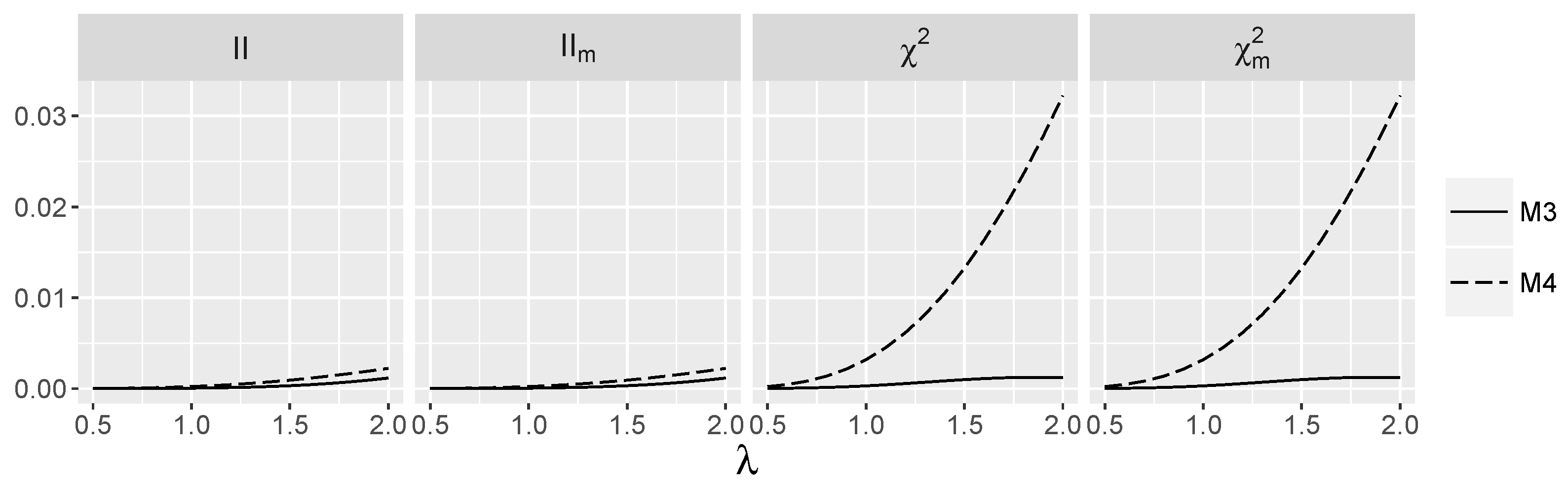
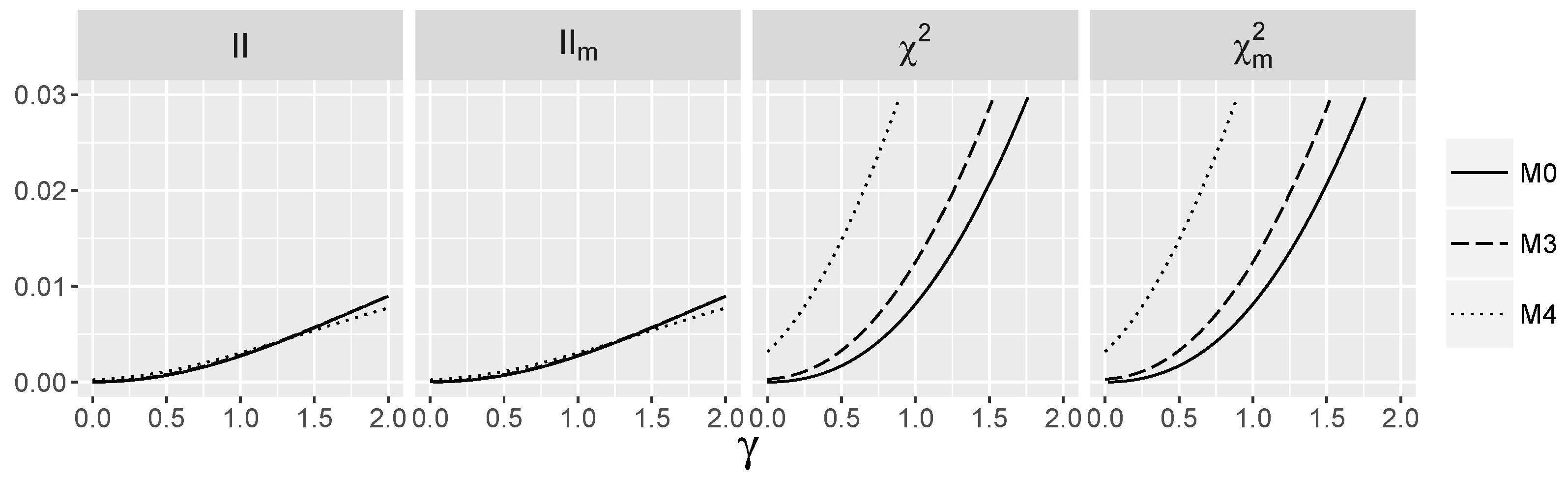
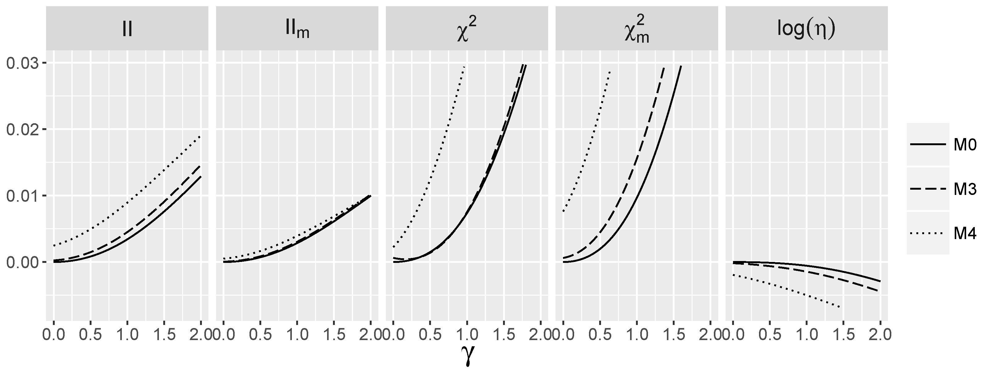
3.3. Behavior of Interaction Indices for Logistic Models

Our main goal here is to check whether estimators of the information interaction lead to satisfactory, universal and easy to compute tests for predictive interaction. We recall that $X_1$ and $X_2$ interact predictively in explaining Y when $II(X_1;X_2;Y)>0.$ Thus, we consider as the null hypothesis $H_0:II=0$ and as an alternative $H_1$, the hypothesis we are interested in, namely $H_1:II>0$. As test statistics, we employ sample versions of interaction information indices and their approximations introduced above. We discuss the behavior of the pertaining tests for logistic models (see Section 3), as for discrete predictors, they cover all possible types of conditional dependence of Y given their values. Two types of distributions of $\left(X_1,X_2\right)$ will be considered, the first, when $X_1$ and $X_2$ are independent and the second one, when their dependence is given by Frank’s copula with parameter $-1$ (see Appendix A for the definition). Frank’s copula with parameter $-1$ was chosen as for the logistic models considered below, it leads to predictive interaction. In both cases, we set Minor Allele Frequency $MAF=0.25$, where $MAF=P(X_1=AA)=P(X_2=BB)$. In

Table A1. Mass function $p\left(x_i,x_j\right)$ of $\left(X_1,X_2\right)$ for $MAF=0.25.$ The upper panel corresponds to independent $X_1$ and $X_2$ and the lower to the Frank copula with $\theta =-1$.

$\mathit{i}\backslash \mathit{j}$	1	2	3	∑
Independent $X_1$ and $X_2$
1	$0.0039$	$0.0235$	$0.0351$	$0.0625$
2	$0.0234$	$0.1406$	$0.2110$	$0.3750$
3	$0.0352$	$0.2109$	$0.3164$	$0.5625$
∑	$0.0625$	$0.3750$	$0.5625$	1
Frank Copula with $\theta =-1$
1	$0.0024$	$0.0180$	$0.0421$	$0.0625$
2	$0.0180$	$0.1232$	$0.2339$	$0.3750$
3	$0.0421$	$0.2339$	$0.2865$	$0.5625$
∑	$0.0625$	$0.3750$	$0.5625$	1

, the conditional distributions are specified (see also Appendix A for the method of generation). As discussed below, larger values of λ and γ lead to larger values of interaction measures.

3.4. Behavior of Interaction Indices When $X_1$ and $X_2$ Are Independent

We consider first a special case when $X_1$ and $X_2$ are independent. We recall that it follows from Proposition 2 (iii) that parameter η then equals one regardless of the form of prevalence mapping. Thus, Kirkwood superposition approximation is a probability distribution, and the fact that $II=0$ is equivalent to the property that distribution P equals its Kirkwood approximation. Moreover, we then have $II=I{I}_m$ and ${\chi }^2={\chi }_m^2.$ We omit the proof of the second equality. Below, we discuss specific logistic regression models that are used in the simulations. For each model, the intercept was set so that prevalence $P(Y=1)$ is approximately $0.1$. In

Table 1. Coefficients for additive logistic models with parameter λ (cf. (39)). In each model, intercept μ was chosen, such that prevalence $P(Y=1)$ is equal to approximately $0.1$.

Model\Coefficients	${\mathit{\alpha }}_1$	${\mathit{\alpha }}_2$	${\mathit{\alpha }}_3$	${\mathit{\beta }}_1$	${\mathit{\beta }}_2$	${\mathit{\beta }}_3$
$M{0}_{\lambda }$	0	0	0	0	0	0
$M{1}_{\lambda }$	λ	0	0	0	0	0
$M{2}_{\lambda }$	λ	λ	0	0	0	0
$M{3}_{\lambda }$	λ	0	0	λ	0	0
$M{4}_{\lambda }$	λ	λ	0	λ	λ	0

, the coefficients for additive logistic models considered here are specified.

Note that for model $M0$, both predictors are independent of Y, whereas in $M1$ and $M2$, only $X_2$ is independent of Y. It is seen from (39) that for $M3$, logarithmic odds depend on the occurrence of either value $AA$, $BB$ or both, whereas for $M4$, they also depend on the values $Aa$ and $Bb$. The additive influence of both loci is the same and measured by parameter λ.

We also consider a general logistic model with interactions given in (40). We employ three types of models, the additive parts of which are the same as in models $M{0}_1,M{3}_1$ and $M{4}_1$, respectively. Note that $M{0}_1$ denotes model $M{0}_{\lambda }$ with $\lambda =1$. The form of interaction is stated in

Table 2. Values of the ${\gamma }_{ij}$ coefficients from Model (40) for the same constant value of $\gamma .$

$\mathit{i}\backslash \mathit{j}$	1	2	3
1	γ	γ	0
2	γ	γ	0
3	0	0	0

. $Mi\left(\gamma \right)$ for $i=0,3,4$ will denote the logistic model, the additive part of which is as in model $M{i}_1$ and interaction part as in Table 2 for a fixed value of $\gamma .$ Thus, $M0(\gamma )$ is a model with no main effects, but with a logistic interaction effect, whereas additive effects, as well logistic interaction are nonzero in $M3(\gamma )$ and $M4(\gamma )$. Note that in the models considered, parameter γ measures the strength of the logistic interaction.

We discuss now how interaction indices behave for the introduced models. We start with additive logistic regression models $M{0}_{\lambda }-M{4}_{\lambda }$. Note that for models $M{0}_{\lambda },M{1}_{\lambda }$ and $M{2}_{\lambda }$, all considered interactions measures are zero, since for $M{0}_{\lambda }$, response Y is independent of $(X_1,X_2)$, whereas for $M{1}_{\lambda }$ and $M{2}_{\lambda }$, predictor $X_2$ is independent of $(X_1,Y)$. The values of $II,I{I}_m,{\chi }^2$ and ${\chi }_m^2$ as a function of λ for models $M{3}_{\lambda }$ and $M{4}_{\lambda }$ are shown in Figure 1.

In models $M{3}_{\lambda }$ and $M{4}_{\lambda }$, the values of $II$ are small, but strictly positive for $\lambda >0$. Note that the monotone dependence of ${\chi }^2={\chi }_m^2$ on λ is much stronger than for $II=I{I}_m$. In Figure 2, the behavior of interaction measures as a function of γ for the logistic model with the nonzero interaction term is depicted. Thus, we check how nonparametric interaction information and its modifications depend on logistic interaction parameter γ. Observe that $II$ is positive, close to zero for $\gamma =0.5$ and for $\gamma \ge 0.5$ grows slowly in all models considered. There is no significant difference between the values of $II$ for all models $M0\left(\gamma \right),M3\left(\gamma \right)$ and $M4\left(\gamma \right)$ when γ is fixed, which means that the additive part in the saturated logistic model has a weak influence on the interaction information. Index ${\chi }^2$ is also approximately 0 for $\gamma =0.5,$ but grows much faster than $II$ when γ increases. The differences between the values of ${\chi }^2$ for models $M0\left(\gamma \right),M3\left(\gamma \right)$ and $M4\left(\gamma \right)$ are much more pronounced than for interaction information $II$, and they increase with $\gamma .$ The values of all indices are larger when the logistic interaction is nonzero.

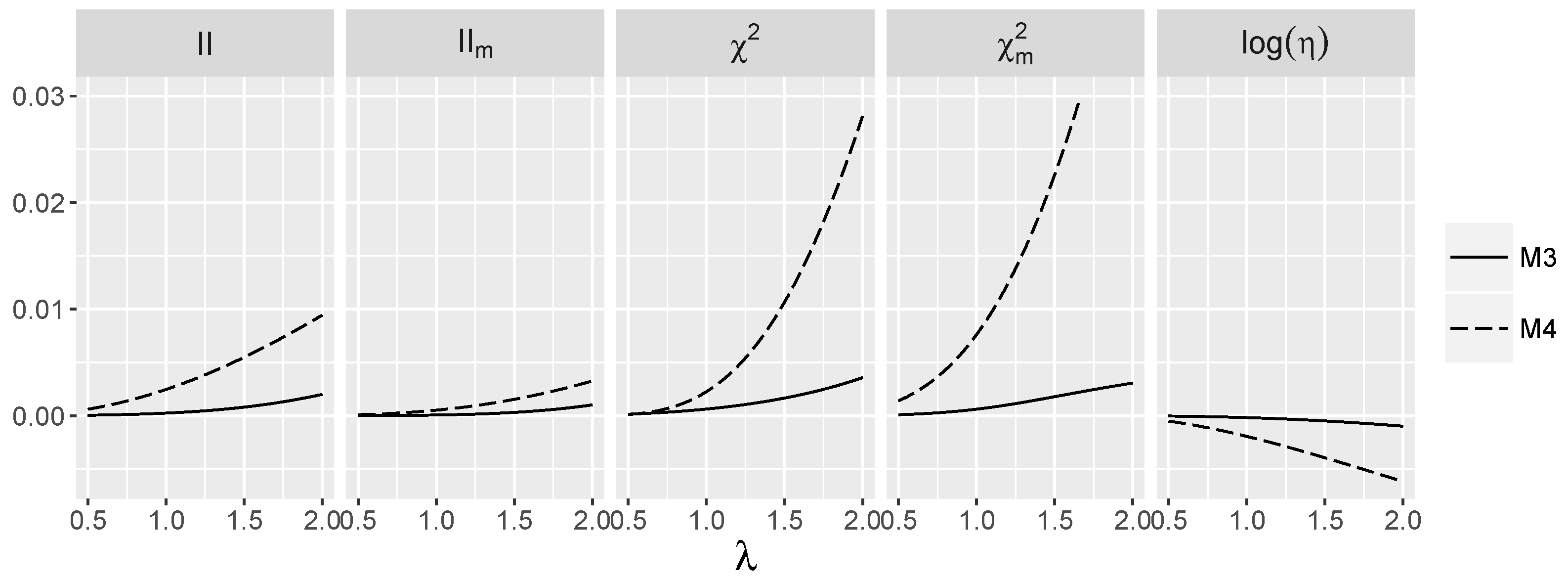
3.5. Behavior of Interaction Indices When $X_1$ and $X_2$ Are Dependent

The situation when $X_1$ and $X_2$ are dependent is more involved. First, Kirkwood superposition approximation does not have to be a probability distribution; therefore, the fact that $II=0$ is not equivalent to the equality of mass functions $p\left(x_i,x_j,y_k\right)$ and ${\tilde{p}}_K\left(x_i,x_j,y_k\right).$ Second, the dependence of predictors means that distribution $(X_1,X_2,Y)$ deviates more strongly from joint independence, i.e., from the situation when the asymptotic behavior of $2n\widehat{II}$ is known and given in (38).

As before, we consider the logistic model with and without interactions. For logistic regression models, we choose the same values of parameters as in the previous section (see Table 1 and Table 2) with the exception of μ, which was set such that in every model, prevalence is equal approximately to $0.1.$

The behavior of interaction indices for the discussed models is shown below. Their variability in λ for models $M{3}_{\lambda },M{4}_{\lambda }$ when predictors are dependent is shown in Figure 3 and for models with interaction in Figure 4. Model $M{0}_{\lambda }$ is omitted as all considered indices are zero there independently of λ. Note that we have a stronger dependence of $II$ on λ in $M4$ than in $M3$; the effect is much weaker in the case of $I{I}_m$ due to the fact that $\log \eta$ negatively depends on λ for M4. Furthermore, for this model, the dependence of $II$ on λ is much stronger than for the independent case.

When logistic interaction is nonzero, we again see pronounced differences in the behavior of $II$ between $M3$ and $M4$. This indicates that in the contrast to the independence case, two factors, namely the value of γ, as well as the form of main effects, influence the value of $II$. The differences between the values of $I{I}_m$ for different models are negligible. Values $II$ are larger for the dependent than for the independent case for the same value of γ. Note that from the logistic model perspective. the strength of interaction in all three models is the same and corresponds to the value of γ. Again, the dependence of ${\chi }^2$ and ${\chi }_m^2$ on γ is much stronger than for $II$.

4. Tests for Predictive Interaction

The main challenge with the application of the constructed statistics for testing is the determination of their behavior under the null hypothesis $II=0$. The asymptotic distribution of $\widehat{II}$ is known only for the case when $X_1,X_2$ and Y are independent, which is a special case only of the null hypothesis, and the asymptotic distributions of ${\widehat{II}}_m$ and $\widehat{\overline{II}}$ are unknown. In order to overcome this problem, we hypothesize that the distributions of all three statistics do not deviate much from the ${\chi }^2(4)$ distribution, at least in the right tails, and we check the validity of our conjecture by calculating the actual Type I error rates for nominal error rates α using the Monte Carlo method. The results are shown in Figure 5 for the independent predictors and in Figure 6 for dependent ones. The results for LRT and ANOVA tests are included as the benchmarks. It is seen that for the independent predictors, discrepancies between actual and nominal rates for $\widehat{II}$ and ${\widehat{II}}_m$ are negligible and comparable to the discrepancy of LRT for all models $M_i,i=0,1,2$, and the same is true for $\widehat{\overline{II}}$ in the case of models $M_0$ and $M_1$. The same observation holds for the dependent predictors, although here, empirical evidence is restricted to model $M_0$, as it is the only model known to us that satisfies the null hypothesis in this case. Based on this observation, in the following, we compare the power of LRT and ANOVA with the powers of the new tests with a rejection region $\{\widetilde{II}\ge {\chi }_{0.95}^2(4)\}$, where ${\chi }_{0.95}^2(4)$ stands for the quantile of order 0.95 of the ${\chi }^2(4)$ distribution and $\widetilde{II}$ stands for either $\widehat{II}$, ${\widehat{II}}_m$ or $\widehat{\overline{II}}$.

Datasets pertaining to the discussed models are generated as described in the Appendix. The pertinent parameters are:

• $t_0,t_1$, the number of observations in controls ($Y=0$) and cases ($Y=1$), set equal in our experiments and $n=t_0+t_1$, the total number of observations. Values of $n=500$ and $n=1000$ were considered.
• MAF, the minor allele frequency for $X_1$ and $X_2$. We set $MAF=0.25$ for both loci.
• copula, the function that determines the cumulative distribution of $\left(X_1,X_2\right)$ based on its marginal distributions.
• $p(i,j):=\mathbb{P}\left(Y=1|x_i,x_j\right)$, the prevalence mapping, which in our experiments was either additive logistic or logistic with nonzero interaction.

For every model, 1000 datasets were generated, and for each of them, tests of the interaction effect based on the introduced indices were performed. The null hypothesis is the lack of predictive interaction $II=0.$ The null hypothesis at the specific significance level α is not rejected if the value of the test statistic is less than $\left(1-\alpha \right)$, the quantile of appropriate distribution; otherwise, we reject this hypothesis and claim that there is a predictive interaction effect. As discussed above, the tests based on all indices except the ANOVA test were compared with the ${\chi }^2\left(4\right)$ distribution, and for the ANOVA test, null distribution was the F-Snedecor distribution with parameters four and $n-9$. For models with $II=0$, we estimate the probability of Type I error for a given α as a fraction of the tests that are falsely rejected. For the model with the predictive interaction effect, statistical power is estimated as a fraction of the tests that are rejected at a significance level of $0.05$. We will refer to those tests as simply interaction information, ${\chi }^2$, LRT and ANOVA tests in the following.

All experiments have been performed in the R environment. The source codes of functions used are available from the corresponding author’s website.

4.1. Behavior of Interaction Tests When $X_1$ and $X_2$ Are Independent

We consider the situation when SNPs $X_1$ and $X_2$ are independent. In this case, $\eta =1$ and both $\widehat{II}$ and ${\widehat{II}}_m$ estimate $II$ consistently.

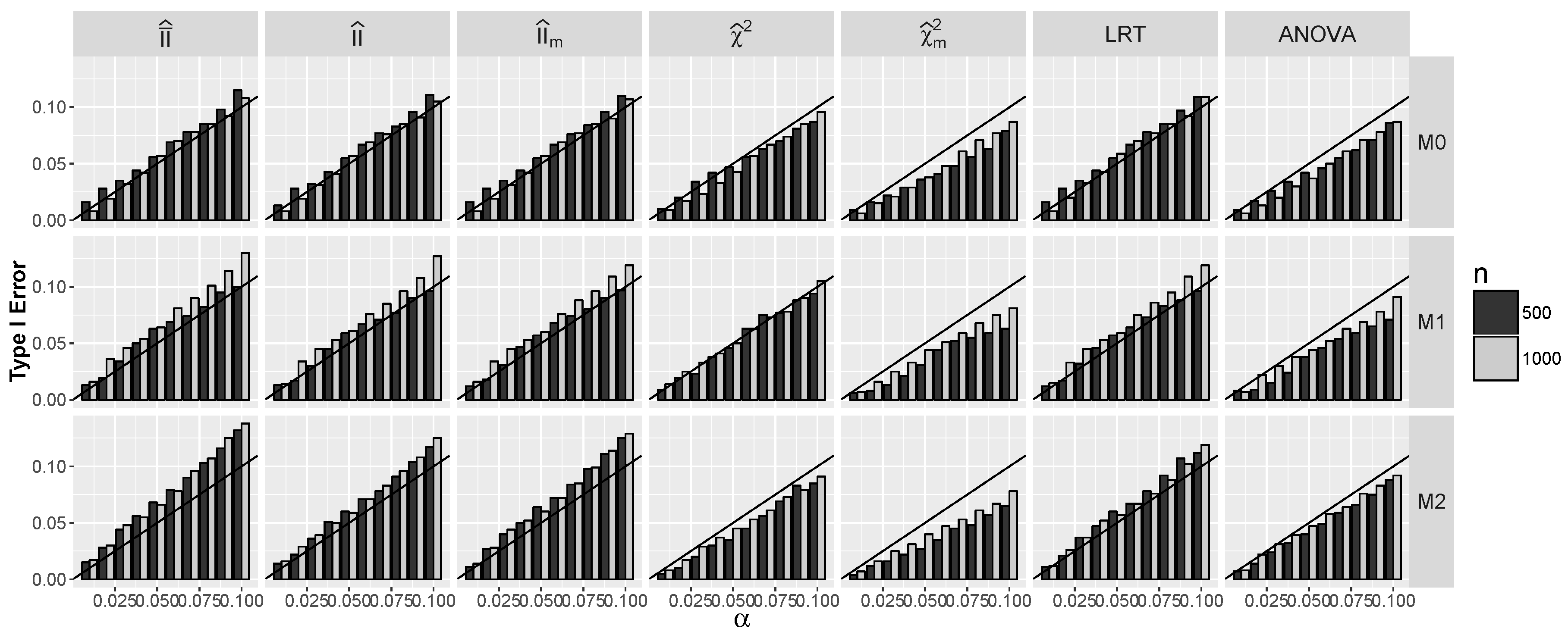
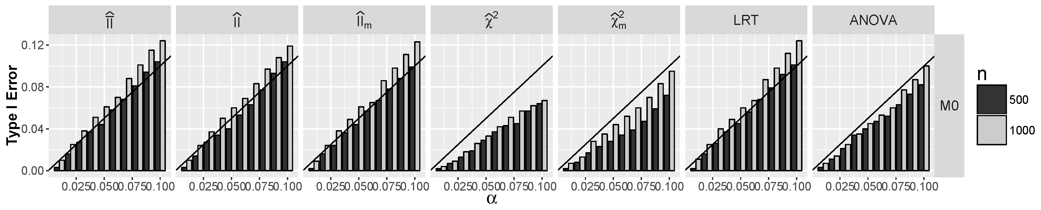
4.1.1. Type I Errors for Models $M0$–$M2$

First, we consider models $M0$–$M2,$ where $II=0$ and for which the null hypothesis holds. Recall that for $M0$, all components of random vector $\left(X_1,X_2,Y\right)$ are independent; thus, in this case, convergence (38) to the ${\chi }^2(4)$ distribution holds. In Figure 5, we compare the Type I error rate with the nominal error rate. Note that Type I errors of $\widehat{II},{\widehat{II}}_m$ and $LRT$ approximately agree with nominal level $\alpha .$ This indicates that the distributions of these statistics under the null hypothesis are approximately ${\chi }^2(4)$ distributed. For ANOVA and ${\chi }^2$ tests, the probability of Type I error is slightly smaller than α. For the maximum statistic $\widehat{\overline{II}}$, the probability of Type I error agrees well with the nominal level for models $M0$ and $M1$ for $M2$; it exceeds α, but the relative difference is not larger than $20\%$ for $\alpha \le 0.05$.

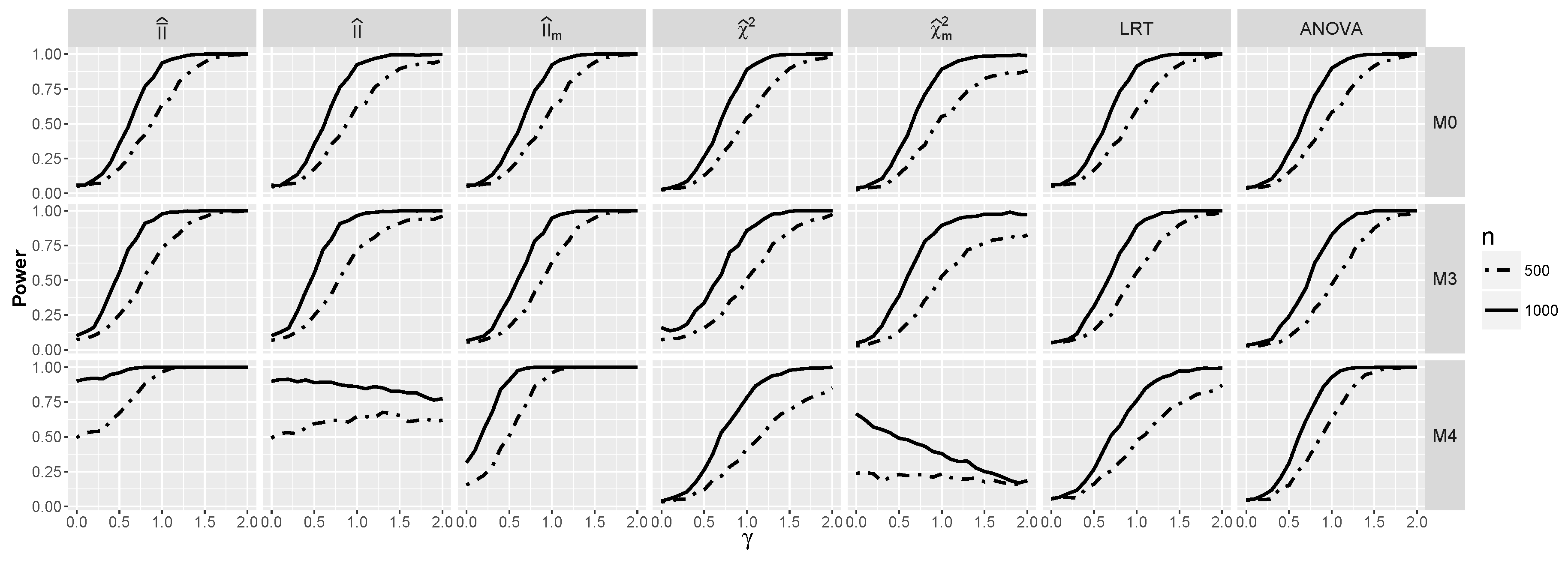
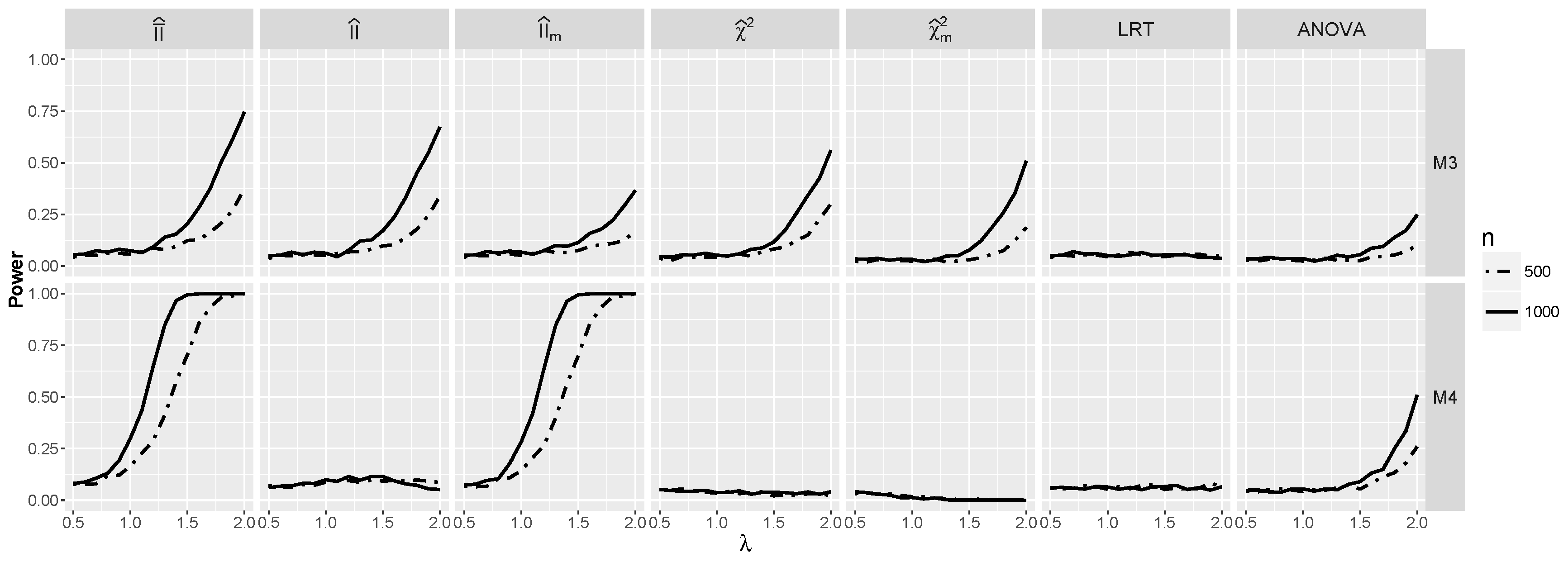
4.1.2. Power for Additive Logistic Models

Now, we focus on models $M{3}_{\lambda }$ and $M{4}_{\lambda }$. From Figure 1, we see that for $\lambda =0.5$, index $II$ is very close to zero, and predictably, the power is close to the significance level for such λ (see Figure 7). However, for larger λ, the power of ${\widehat{II}}_m$ and $\widehat{II}$ increases for $M3$, and in the case of $M4$, this holds also for ${\widehat{II}}_m$. The difference between the behavior of ${\widehat{II}}_m$ on the one side and $\widehat{II}$ and ${\chi }^2$ approximations on the other for model $M4$ is remarkable and shows that modification incorporating $\log \widehat{\eta }$ is worthwhile. However, for model $M3$, it does not improve the performance of $\widehat{II}$. Note also that unsurprisingly. The power of the $LRT$ test stays close to the significance level, but the power of ANOVA starts to increase for large λ. A clear winner in both cases is the test based on $\widehat{\overline{II}}$, which performs very well for both models, as it takes advantage of the good performance of $\widehat{II}$ for $M3$ and ${\widehat{II}}_m$ for model $M4$.

4.1.3. Power for the Logistic Model with Interactions

We consider now the power of the tests with respect to logistic interaction parameter γ for models $M0\left(\gamma \right),M3\left(\gamma \right)$ and $M4\left(\gamma \right).$ Note that $M0\left(\gamma \right)$ is now included as $II$ is positive for $\gamma >0$. In all cases, ${\widehat{II}}_m$ performs better than $\widehat{II}$, supporting the usefulness of the correction. $LRT$ works comparably to ANOVA and, in some cases, worse than ${\widehat{II}}_m$ and $\widehat{\overline{II}}$. We stress that this does not contradict the fact that $LRT$ is the most powerful test at the level α for null hypothesis ${\overline{H}}_0:\gamma =0$. Indeed, it follows from the previous experiments that predictive interaction tests are not level α tests for ${\overline{H}}_0$; thus, they may have larger power than $LRT$. The power of ${\widehat{II}}_m$ and $\widehat{\overline{II}}$ is around $30\%$ for $M4$, even for γ close to zero, when for $LRT$, it stays around a significance level of 0.05. Note also that $\widehat{II}$ and ${\widehat{\chi }}_m^2$ fail to detect the predictive interaction for model $M4$.

4.2. Behavior of the Interaction Tests When $X_1$ and $X_2$ Are Dependent

We consider the situation where SNPs $X_1$ and $X_2$ are dependent. The distribution of $\left(X_1,X_2\right)$ is modeled by the Frank copula with $\theta =-1$ (see Table A1).

4.2.1. Type I Errors for Model $M0$

Note that for dependent $X_1$ and $X_2$, only $M0$ satisfies the null hypothesis, as for the models $M1$ and $M2$, index $II$ is negative. It follows from Figure 6 that for all tests apart from ${\chi }^2$ tests, Type I error for $M0$ is approximately α, and it is significantly smaller than α for both ${\chi }^2$ tests. For larger α and $n=1000$ errors for information, interaction tests exceed slightly α, similarly to LRT.

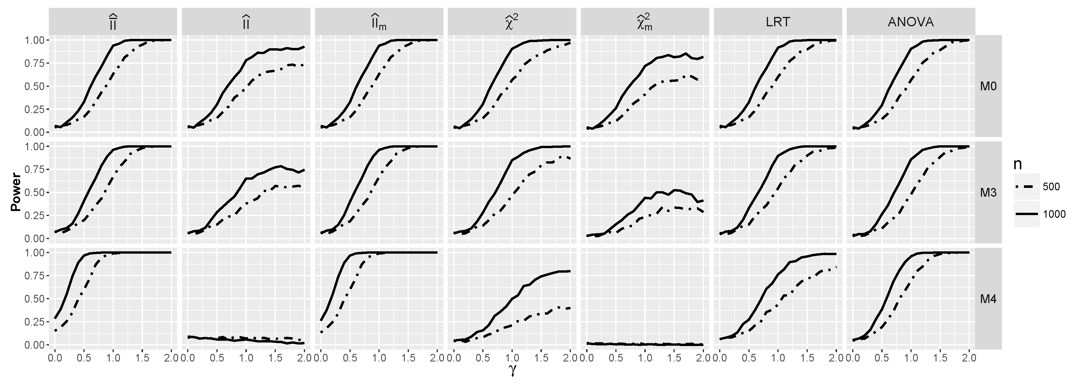
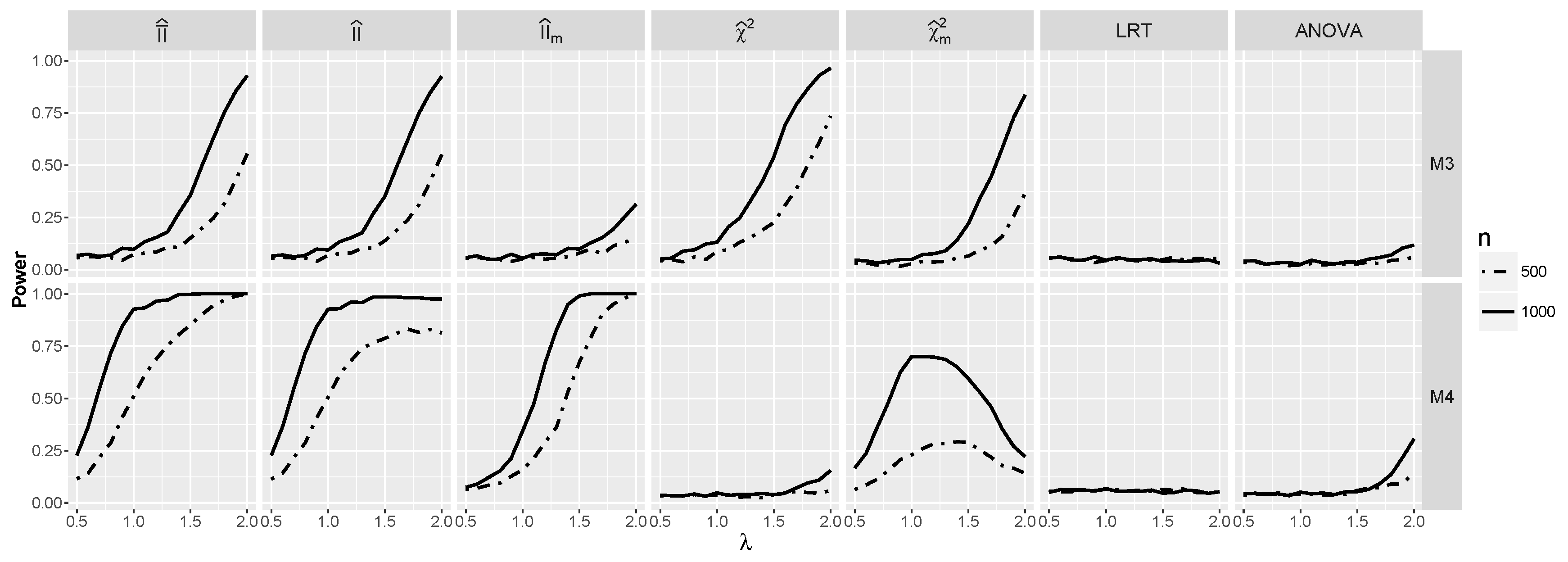
4.2.2. Power for Additive Logistic Models When $X_1$ and $X_2$ Are Dependent

The behavior of the discussed tests is analogous to the case of independence (see Figure 8) with one important difference. Namely, now $\widehat{II}$ performs better than ${\widehat{II}}_m$ apart from model $M4$ for $\lambda \ge 1.5$ and $n=500$. $LRT$ and ANOVA do not detect any interaction for $\lambda \le 1.5$, but the power of ANOVA starts to pick up for large λ. Note the erratic behavior of the ${\widehat{\chi }}_m^2$ test for which the power actually starts to decrease for larger λ. This possibly is caused by the fact that the test is not well calibrated and the fact that ${\widehat{\chi }}_m^2$ is likely to become negative for large λ. The power of $\widehat{\overline{II}}$ is the largest one among all tests.

4.2.3. The Powers for Logistic Models with Interaction When $X_1$ and $X_2$ Are Dependent

Obviously, when logistic interaction is present, the $LRT$ test performs much better (see Figure 9). The same applies to ANOVA and $\widehat{II}$, but the best performance is again exhibited by $\widehat{\overline{II}}$. Consider, e.g., its performance for the model $M4$. Its excellent behavior for small γ’s stems from the very good performance of $\widehat{II}$, whereas for larger γ’s from the performance of ${\widehat{II}}_m.$ Comparing Figure 9 and Figure 10, we see that the dependence between predictors improved the performance of the tests based on the interaction information measures, especially for a smaller sample size, which is consistent with the larger values of the interaction information in the dependent than in the independent case. Note that in the dependent case, the power of $\widehat{II}$ and $\widehat{\overline{II}}$ for $M4$ is above $0.9$ for γ close to zero, whereas it is less then $0.3$ for such γ in the independent case.

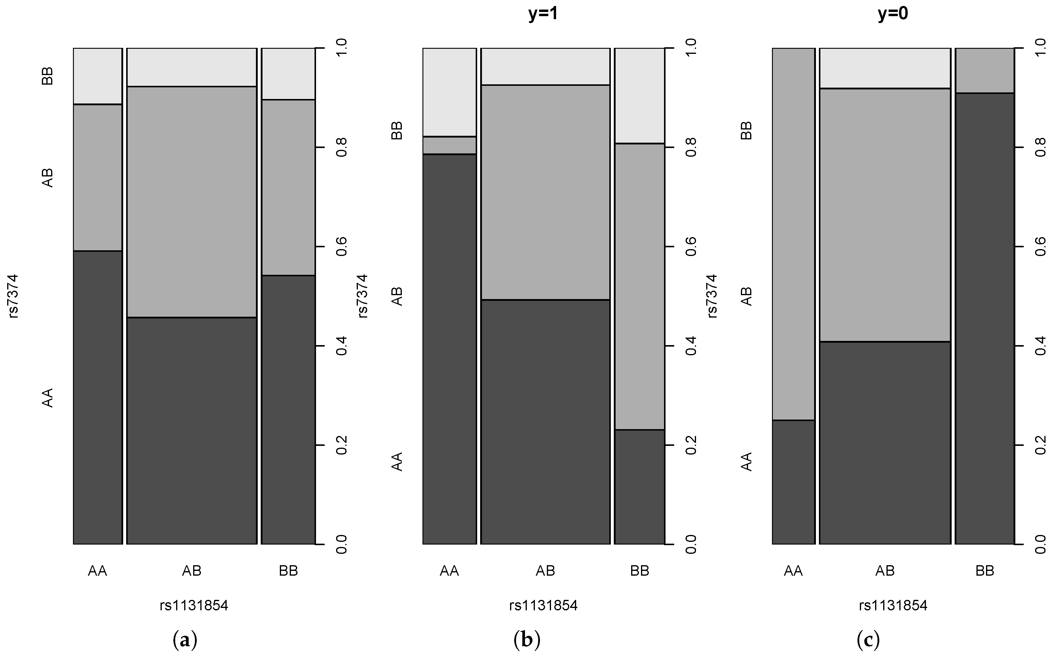
4.3. Real Data Example

We perform the analysis of a real dataset in order to show that the pairs of SNPs that correspond to large values of interaction indices exhibit interesting patterns of conditional dependence. We used data on pancreatic cancer studied by [27] and downloaded from the address [28]. They consist of 208 observations (121 cases and 87 controls) with values of 901 SNPs. We applied tests $\widehat{II}$, ${\widehat{II}}_m$ and $\widehat{\overline{II}}$ for all pairs and $\alpha =0.05$ with Bonferroni correction resulting in an individual level of significance $1.23\times {10}^{-7}=0.05/K$, where $K=(901\times 900)/2$. All three tests rejected the null hypothesis $II=0$ for 11 pairs. The pair of SNPs with the largest values of $\widehat{II}$ and ${\widehat{II}}_m$ is the pair $(SNP1,SNP2)=$(rs1131854,rs7374) with values $\widehat{II}=0.1239$ and ${\widehat{II}}_m=0.1246$. Figure 11 shows the probability mass function of this pair (a) and of the conditional mass functions given $Y=1$ (b) and $Y=0$ (c).

Note that the pattern of the change of the conditional probabilities of the occurrence of the AA genotype for SNP2 given the genotypes of SNP1 for the cases $Y=1$ is reversed in the case of the controls $Y=0$. For the pooled sample, the conditional probabilities are approximately equal. Moreover, observe that the conditional frequency of $SNP2=BB$ given $SNP1=BB$ is around 0.2 for the cases, whereas it is zero for the controls.

This preliminary example indicates that the analysis based on large values of interaction information indices allows one to detect interesting patterns of dependence between pairs of SNPs and the response.

5. Discussion

In the theoretical part of the paper, we reviewed and proved some new properties of interaction information, its modification and their approximations. It is argued that parameter η introduced in (11) plays an important role in establishing predictive interaction. Theoretical analysis supported considering a new measure defined in (16), being the maximum of interaction information, and its modified version, which was considered in numerical experiments. There are several conclusions that can be drawn from the conducted numerical experiments. The first one is that the dependence between predictors influences the performance of interaction information tests: while ${\widehat{II}}_m$ performs in general better than $\widehat{II}$ for independent predictors, the situation is reversed for dependent ones. Their natural combination, statistics $\widehat{\overline{II}}$, is superior to any of them and $LRT$. When compared to $LRT$, the difference in performance is most striking when detecting predictive interaction in the cases when logistic interaction is 0 as, e.g., in models $M{3}_{\lambda }$ and $M{4}_{\lambda }$. This should serve as a cautionary remark for the situations when the interaction information test is used as a screening test and then LRT is applied for remaining pairs of genes: the screening test may rightly retain pairs of genes interacting predictively; however, the interaction may not be confirmed by the $LRT$ test. Such cases are likely to occur especially for dependent pairs. It is also worthwhile to note that $\widehat{\overline{II}}$ is as least good as $LRT$ and sometimes much better for detecting interactions when the logistic interaction γ is close to zero. This is a promising feature, as detecting such weak interactions is the most challenging and bears important consequences for revealing the dependence structure of diseases. This of course requires the construction of interaction tests suitable for a huge number of pairs and is a subject of further study. On the negative side, tests based on ${\chi }^2$ approximations tend to perform less well than those based on interaction information and their modifications. This is possibly due to their non-adequate calibration in the case when the null hypothesis holds. It also should be stressed that in numerical experiments, we studied the problem of distinguishing between no interaction information ($II=0$) and predictive interaction ($II>0$). In the case when interaction information is negative, ${\widehat{II}}_m$ and $\widehat{\overline{II}}$ are likely not to detect such an effect.

References

- Cordell, H.J. Epistasis: What it means, what it doesn’t mean, and statistical methods to detect it in humans. Hum. Mol. Genet. 2002, 11, 2463–2468. [Google Scholar] [CrossRef]
- Ritchie, M.; Hahn, L.; Roodi, N.; Bailey, L.; Dupont, W.; Parl, F.; Moore, J. Multifactor dimensionality reduction reveals high-order interactions in genome-wide association studies in sporadic breast cancer. Am. J. Hum. Genet. 2001, 69, 138–147. [Google Scholar] [CrossRef] [PubMed]
- Zhang, J.; Liu, R. Bayesian inference of epistatic interactions in case-control studies. Nat. Genet. 2007, 39, 167–173. [Google Scholar] [CrossRef] [PubMed]
- Yang, C.; He, Z.; Wan, X.; Yang, Q.; Xue, H.; Yu, W. SNP Harvester: A filtering-based approach for detecting epistatic interactions in genome-wide association studies. Bioinformatics 2009, 25, 504–511. [Google Scholar] [CrossRef] [PubMed]
- Liu, Y.; Xu, H.; Chen, S. Genome-wide interaction based association analysis identified multiple new susceptibility loci for common diseases. PLoS Genet. 2011, 7, e1001338. [Google Scholar] [CrossRef] [PubMed]
- Goudey, B.; Rawlinson, D.; Wang, Q.; Shi, F.; Ferra, H.; Campbell, R.M.; Stern, L.; Inouye, M.T.; Ong, C.S.; Kowalczyk, A. GWIS—Model-free, fast and exhaustive search for epistatic interactions in case-control GWAS. BMC Genom. 2013, 14 (Suppl. 3), S10. [Google Scholar] [CrossRef] [PubMed]
- Chanda, P.; Sucheston, L.; Zhang, A.; Brazeau, D.; Freudenheim, J.; Ambrosone, C.; Ramanathan, M. AMBIENCE: A novel approach and efficient algorithm for identifying informative genetic and environmental associations with complex phenotypes. Genetics 2008, 180, 1191–1210. [Google Scholar] [CrossRef] [PubMed]
- Wan, X.; Yang, C.; Yang, Q.; Xue, T.; Fan, X.; Tang, N.; Yu, W. BOOST: A fast approach to detecting gene-gene interactions in genome-wide case-control studies. Am. J. Hum. Genet. 2010, 87, 325–340. [Google Scholar] [CrossRef] [PubMed]
- Wei, W.H.; Hermani, G.; Haley, C. Detecting epistasis in human complex traits. Nat. Rev. Genet. 2014, 15, 722–733. [Google Scholar] [CrossRef] [PubMed]
- Moore, J.; Williams, S. Epistasis. Methods and Protocols; Humana Press: New York, NY, USA, 2015. [Google Scholar]
- Duggal, P.; Gillanders, E.; Holmes, T.; Bailey-Wilson, J. Establishing an adjusted p-value threshold to control the family-wide type 1 error in genome wide association studies. BMC Genom. 2008, 9, 516. [Google Scholar] [CrossRef] [PubMed]
- Culverhouse, R.; Suarez, B.K.; Lin, J.; Reich, T. A perspective on epistasis: Limits of models displaying no main effect. Am. J. Hum. Genet. 2002, 70, 461–471. [Google Scholar] [CrossRef] [PubMed]
- Lüdtke, N.; Panzeri, S.; Brown, M.; Broomhead, D.S.; Knowles, J.; Montemurro, M.A.; Kell, D.B. Information-theoretic sensitivity analysis: A general method for credit assignment in complex networks. J. R. Soc. Interface 2008, 5, 223–235. [Google Scholar] [CrossRef] [PubMed]
- Evans, D.; Marchini, J.; Morris, A.; Cardon, L. Two-stage two-locus models in genome-wide asssociation. PLoS Genet. 2006, 2, 1424–1432. [Google Scholar]
- McGill, W. Multivariate information transmission. Psychometrika 1954, 19, 97–116. [Google Scholar] [CrossRef]
- Fano, F. Transmission of Information: Statistical Theory of Communication; MIT Press: Cambridge, MA, USA, 1961. [Google Scholar]
- Cover, T.; Thomas, J. Elements of Information Theory; Wiley: New York, NY, USA, 2006. [Google Scholar]
- Han, T.S. Multiple mutual informations and multiple interactions in frequency data. Inf. Control 1980, 46, 26–45. [Google Scholar] [CrossRef]
- Kang, G.; Yue, W.; Zhang, J.; Cui, Y.; Zuo, Y.; Zhang, D. An entropy-based approach for testing genetic epistasis underlying complex diseases. J. Theor. Biol. 2008, 250, 362–374. [Google Scholar] [CrossRef] [PubMed]
- Zhao, J.; Jin, L.; Xiong, M. Test for interaction between two unlinked loci. Am. J. Hum. Genet. 2006, 79, 831–845. [Google Scholar] [CrossRef] [PubMed]
- Darroch, J. Interactions in multi-factor contingency tables. J. R. Stat. Soc. Ser. B 1962, 24, 251–263. [Google Scholar]
- Sucheston, L.; Chanda, P.; Zhang, A.; Tritchler, D.; Ramanathan, M. Comparison of information-theoretic to statistical methods for gene-gene interactions in the presence of genetic heterogeneity. BMC Genom. 2010, 11, 487. [Google Scholar] [CrossRef] [PubMed]
- Darroch, J. Multiplicative and additive interaction in contingency tables. Biometrika 1974, 9, 207–214. [Google Scholar] [CrossRef]
- Li, W.; Reich, J. A complete enumeration and classification of two-locus disease models. Hum. Hered. 2000, 17, 334–349. [Google Scholar] [CrossRef]
- Culverhouse, R. The use of the restricted partition method with case-control data. Hum. Hered. 2007, 63, 93–100. [Google Scholar] [CrossRef] [PubMed]
- Rencher, A.C.; Schaalje, G.B. Linear Models in Statistics; Wiley: Hoboken, NJ, USA, 2008. [Google Scholar]
- Tan, A.; Fan, J.; Karakiri, C.; Bibikova, M.; Garcia, E.; Zhou, L.; Barker, D.; Serre, D.; Feldmann, G.; Hruban, R.; et al. Allele-specific expression in the germline of patients with familial pancreatic cancer: An unbiased approach to cancer gene discovery. Cancer Biol. Ther. 2008, 7, 135–144. [Google Scholar] [CrossRef]
- SNPsyn. Available online: http://snpsyn.biolab.si (accessed on 4 January 2017).
- Nelson, R.B. An Introduction to Copulas; Springer: New York, NY, USA, 1999. [Google Scholar]
Figure 1.
Theoretic values of interaction measures for the additive logistic model and independent SNPs.
Figure 2.
Theoretic values of the interaction measures for the logistic model with the interaction and independent SNPs.
Figure 3.
Theoretic values of the interaction measures for the additive logistic model and dependent SNPs.
Figure 4.
Theoretic values of the interaction measures for the logistic model with the interaction and dependent SNPs.
Figure 5.
Actual Type I error rates against the nominal error α rate when and are independent for models and
Figure 6.
Actual Type I error rates against nominal error rate α when and are dependent for model
Figure 7.
Powers for models and against λ when and are independent.
Figure 8.
Powers for models and against λ when and are dependent.
Figure 9.
The power for models and against γ when and are dependent.
Figure 10.
Powers for models and against γ when and are independent.
Figure 11.
Probability mass function for the pair (rs1131854,rs7374) (a) and for corresponding conditional mass functions given (b) and (c).