Combined Forecasting of Streamflow Based on Cross Entropy

Abstract

In this study, we developed a model of combined streamflow forecasting based on cross entropy to solve the problems of streamflow complexity and random hydrological processes. First, we analyzed the streamflow data obtained from Wudaogou station on the Huifa River, which is the second tributary of the Songhua River, and found that the streamflow was characterized by fluctuations and periodicity, and it was closely related to rainfall. The proposed method involves selecting similar years based on the gray correlation degree. The forecasting results obtained by the time series model (autoregressive integrated moving average), improved grey forecasting model, and artificial neural network model (a radial basis function) were used as a single forecasting model, and from the viewpoint of the probability density, the method for determining weights was improved by using the cross entropy model. The numerical results showed that compared with the single forecasting model, the combined forecasting model improved the stability of the forecasting model, and the prediction accuracy was better than that of conventional combined forecasting models.

1. Introduction

Streamflow prediction is essential for the rational development and utilization of water resources. However, due to the effects of rainfall, the geographical environment, and human activities, streamflow exhibits high volatility and randomness, and thus its prediction is very complex and difficult. Previous studies of streamflow prediction have employed approaches such as time series methods [1,2], grey modeling [3], regression analysis [4], wavelet analysis [5], Markov chain modeling [6], and neural networks [7,8,9]. Single methods are simple, but the impact of abnormal data or fluctuations over time may cause significant errors, so their reliability is not high. In recent years, the prediction method has been improved in many studies. In [10], the multivariate ensemble streamflow prediction was employed, where a variety of meteorological factors were used as input variables for training to obtain the prediction results. This method considers the diversity of historical data. In [11], functional linear models were introduced and applied to hydrological forecasting to forecast the whole flow curve instead of points (daily or hourly). This method is an improvement of the traditional regression model, which is more concerned with the stability of the overall prediction process. In [12], Sobol’s variance-based sensitivity analysis was used to rank the model parameters based on their influence on the model results, thereby determining the optimal hydrological model parameters and predictions were then obtained. Thus, the improved methods mainly include data mining, algorithm improvement, and parameter optimization. However, forecasting methods based on historical data are highly dependent on the samples and when the data are unstable, the forecasting method cannot be guaranteed to perform accurately at all points.

In 1969, Bates and Granger proposed a combined forecasting method based on weights [13], which can combine different methods and data features to improve the accuracy of forecasting and reduce the risk of the model failing. At present, there are two main types of combined forecasting methods: in the one-step method, two or more models are integrated to obtain an improved forecasting method, such as a combined random and gray integration method, or the linking of fuzzy and neural network analysis to produce a fuzzy neural network [14], although this is not pure combined forecasting; and the other type comprises parallel methods, where the forecasting results obtained by multiple single methods are weighted according to certain rules. In this study, we consider the second type of method. In [15,16], the objective function was weighted by the minimum sum of the squares of the forecast errors, but the time characteristics of the data were not considered adequately. In [17], based on the selection of a similar day, a neural network method was used for dynamic weighting, but the neural network algorithm was not adequate and it was readily trapped by a local optimal solution, while the number of calculations was high.

The concept of entropy, which was proposed by the German physicist Clausius in 1877, is a function of the state of the system, where a reference value and the variation in entropy are often analyzed and compared. Cross entropy (CE) is a type of entropy that reflects the similarity between variables from the perspective of probability. In recent years, some studies have applied CE to the field of hydrology. Entropy theory was introduced in [18] and applied to environmental and water engineering, including water resource evaluation, variable correlation, and reliability evaluation. A new entropy-based approach was also developed for deriving a 2D velocity distribution in an open-channel flow to investigate a rectangular geometric domain and a reliable estimation [19,20]. In addition, CE was introduced into combined forecasting [21,22], where a new method was proposed for determining weights to improve the stability of the prediction results. However, the probability density function used in [21] is not suitable for predicting a radial flow. In addition, a wind power load forecasting method based on the normal distribution was proposed by [22], but the time characteristics of the historical data were not considered and the solution process was complex.

In this study, we combine the autoregressive integrated moving average (ARIMA), improved grey forecasting model (GM), and an artificial neural network (a radial basis function, RBF) in a single forecasting model. Based on the time effectiveness of historical data, we develop a combined forecasting method based on CE. The Lagrange function method is used to solve the problem, which is based on the prediction error of a single method for adjusting the weights, so the predicted results are more consistent with the actual situation, thereby improving the accuracy and stability of predictions.

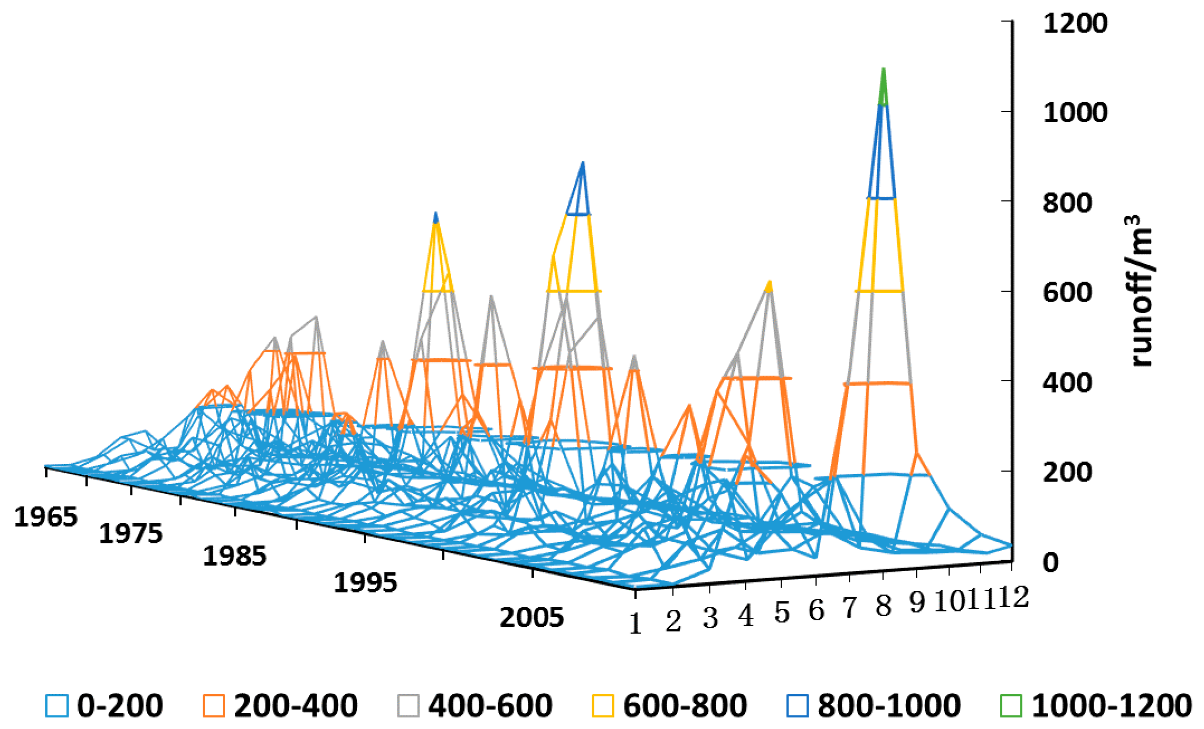
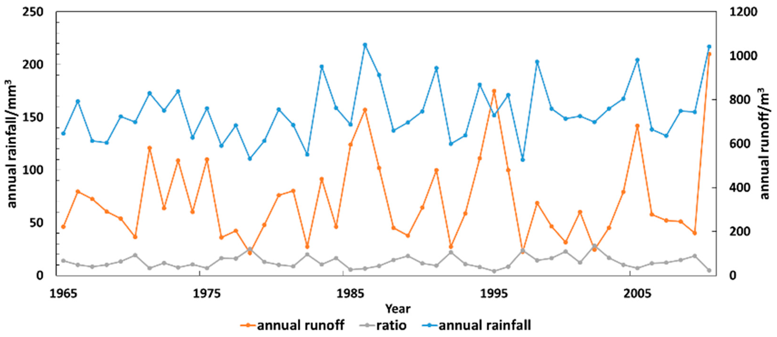
2. Analysis of Streamflow Characteristics

The Huifa River arises in the Longgang Mountains of Qingyuan Manchu Autonomous County, Fushun City, Liaoning Province, Northeast China, and it flows for 33.70 km into Jilin Meihekou City, Huinan County, and Panshi City. The Huifa River is the largest tributary of the second Songhua River. Its watershed area is 14,896 km² and it is located mainly in the territory of Jilin. According to data obtained at the Wudaogou hydrology station in Huadian City (catchment area of 12,391 km²), the change in the amplitude of its water level is 7.69 m, the average annual streamflow is 26.4 billion m³, the average flow is 83.70 m³/s, the maximum peak discharge is 3010 m³/s (1975), the minimum flow rate is 0.44 m³/s (1979), the mean annual sediment volume is 0.48 kg/s, and the annual transportation of sediment is 121 million metric tons.

Figure 1 shows the changes in the streamflow at Wudaogou hydrological station during 1965–2010. It can be seen that the monthly streamflow usually increases from January and it generally reaches a peak in July or August, before exhibiting a declining trend until the end of the year. In addition to the extreme streamflow during the flood season in some individual years (e.g., 938 m³ in 1995 and 1080 m³ in 2010), the trend and the actual numerical value of the monthly streamflow are relatively strong in each year. Therefore, the selection of reasonably similar years can improve the accuracy of streamflow predictions.

Previous studies (e.g., [23]) indicate that rainfall is the main source of streamflow and, thus, the rainfall and flow should have a strong correlation. In order to verify this, we show the annual streamflow and annual rainfall during 1965–2010, as well as the ratio of the two curves in Figure 2.

Figure 2 shows that the trends in the annual streamflow and annual rainfall variation are highly similar, except in some individual years (1986, 1995, and 2010). We conducted a regression analysis of the data and used SPSS software (v19.0, IBM Corp., Armonk, NY, USA) to calculate the R2, which was significant at R2 = 0.921, thereby demonstrating that the streamflow and rainfall had a strong correlation. Thus, the historical rainfall data can be used as an input variable [9] to improve the accuracy of forecasting. The forecast rainfall value can also be used for streamflow forecasting in similar years, thereby making the use of historical data more scientific.

3. Data Processing Method

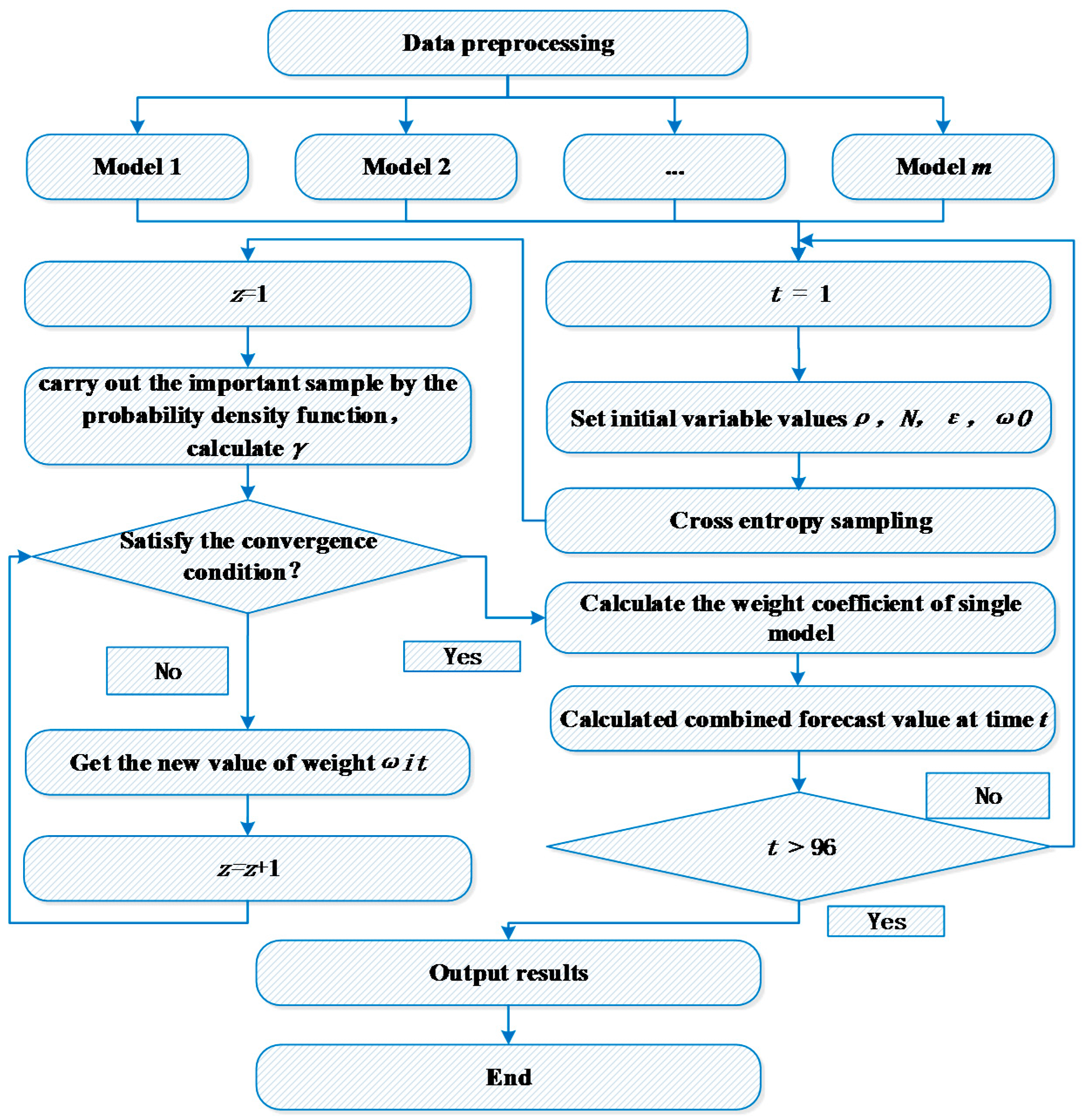
3.1. Data Preprocessing

Data preprocessing involves the processing of missing data and data normalization. In the proposed method, we use linear interpolation to fill in any missing data. If the streamflow value is $L_t$ at time t and $L_{t+a\Delta t}$ at time t + aΔt, and the streamflow data are missing at the intermediate time t + bΔt, then the missing values can be expressed as follows:

$$L_{t+b\Delta t}=L_t+b\times \frac{L_{t+b\Delta t}-L_t}{a},b<a$$

(1)

The dimensions of the various types of data are different, so it is necessary to normalize the historical data, and the normalized processing of the streamflow data is conducted as follows:

$$x^{\prime }=0.1+0.8\frac{x}{x_{\max }}$$

(2)

where x’ is the normalized value, x is the value at a certain time, and x_max is the maximum value in the sample.

3.2. Selecting Similar Years

Selecting reasonably similar years can improve the accuracy of predictions. Many methods can be employed for this purpose, including evidence theory, clustering analysis, the trend similarity method, and the grey correlation method. We use the gray correlation degree to select similar years.

The factor considered in this study is the rainfall value, so the training samples and the forecast years have highly similar characteristics. We calculate the historical date sequence:

$$X_{m_0}=\left(x_{m_0}\left(1\right),\dots ,x_{m_0}\left(g\right)\right)\left(m_0=1,\dots ,n\right)$$

(3)

and the predicted date sequence:

$$X_0=\left(x_0\left(1\right),\dots ,x_0\left(g\right)\right)$$

(4)

where the correlation degree g is the number of factors included.

First, we obtain the maximum difference value and the minimum difference value, as follows:

$${\Delta }_{\min }=\min \min (\Delta )$$

(5)

$${\Delta }_{\max }=\max \max (\Delta )$$

(6)

We then calculate the gray correlation degree between X₀ and Xm₀:

$$r\left(X_0,X_{m_0}\right)=\frac{1}{g}{\displaystyle \sum _{k=1}^g\frac{{\Delta }_{\min }+\rho {\Delta }_{\max }}{{\Delta }_{m0}\left(k\right)+\rho {\Delta }_{\max }}}$$

(7)

where ρ is the resolution coefficient, which is defined as 0.5 in this study: ${\Delta }_{m0}=(|x_{m_0}(1)-x_0(1)|,\dots ,|x_{m_0}(g)-x_0(g)|)$. If we set a threshold for r, then we can obtain the similar years based on the threshold, before using these data for modeling and calculations.

4. Streamflow Forecasting Model Based on CE

4.1. Combined Forecasting Model

The combined forecasting model comprises m single forecasting models and the relative effectiveness of a single forecasting model determined by the historical data. If the combined forecast value at time t is y_t, ${\omega }_{it}$ is the weight of the ith model at time t, and ${\widehat{y}}_{it}$ is the predicted value of the ith model at time t, then the problem of combined forecasting is described as follows:

$$y_t={\displaystyle \sum _{i=1}^m{\omega }_{it}{\widehat{y}}_{it}}$$

(8)

where ${\displaystyle \sum _{i=1}^m{\omega }_{it}}=1$. From Equation (8), we can know that two factors influence the final results of combined forecasting: a single model and the weight of a single forecasting model. In this study, we focus on the latter.

There are no uniform rules for selecting a single method, but instead we must consider the actual problem and the needs of the model. The factors considered in this study include: independence, diversity, and the accuracy of the algorithm. We use a single forecasting method to include the ARIMA time series model, GM, and the RBF. Due to limitations on the length of this report, we give no detailed introduction, but readers may refer to previous studies [12,24,25].

The ARIMA model parameters (p, q, d) are obtained from the lowest order ARIMA (1, 1, 1) model, and the minimum Akaike’s information criterion is used to find the optimal parameters, where p = 2, q = 3, and d = 2 are used in the prediction model. The GM prediction model is based on the selection of similar years (see Section 3.2). In the RBF prediction model, the input variables comprise the historical streamflow and rainfall data predicted for a five-year period by network training, where the output variable predicts the annual streamflow.

4.2. The CE Model

According to the definition of entropy, a method for calculating the difference in information between two random vectors is defined as the CE. The CE model can determine the extent of the mutual support degree by assessing the degree of intersection between different information sources. In addition, the mutual support degree can be used to determine the weights of the information sources, where a greater weight represents higher mutual support [26]. This is also called the Kullback–Leibler (K-L) distance. The CE of two probability distributions is expressed as D(f || g).

For the discrete case:

$$D(g||f)={\displaystyle \sum _1^n{g}_i\ln \frac{g_i}{f_i}}$$

(9)

and for the continuous case:

$$D(g||f)={\displaystyle \int g(x)}\ln \frac{g(x)}{f(x)}dx={\displaystyle \int g(x)}\ln g(x)dx-{\displaystyle \int g(x)}\ln f(x)dx$$

(10)

where f and g denote the probability vector in the discrete case and the probability density function in the continuous case, respectively.

The CE model quantifies the “distance” between the amounts of information. However, the K-L distance is not the real length distance, but instead it is the difference between two probability distributions. CE value should be smallest when two pdfs are identical. For the combined forecasting model based on CE, the CE model represents the support for combined forecasting. Therefore, the objective is to assign weights to two different individual methods, so the most similar result is obtained between the total predictive function and the true value.

Using the CE model should solve two major problems: establishing the probability density function and generating the CE objective function, and solving the weight coefficient by iteration.

The streamflow is treated as a sequence of discrete random variables in the forecast period. For a certain point in the sequence, the value of the streamflow at a certain prediction time is continuous, so it can be regarded as a continuous random variable. Therefore, streamflow prediction can be treated as a sequence of discrete times but continuous values.

The probability density function for predicting streamflow f(x) can be regarded as the probability density function $f_i(x)$ of the single forecasting method multiplied by the corresponding weight. According to the central limit theorem [22], if a variable is influenced by many small independent random factors, then we can treat the variable as following a normal distribution and, thus, the streamflow value at a certain time can be considered as satisfying a normal distribution. The minimum CE is used to determine the probability distribution of the different forecasting methods, so the combined probability distribution of the streamflow is obtained.

The probability density function for method i is (i = 1,2,…,m):

$$f_i(x)=\frac{1}{\sqrt{2\pi }{\sigma }_i}{e}^{-{(\mathrm{x}-{\mu }_i)}^2/(2{\sigma }_i^2)}$$

(11)

where ${\mu }_i$ is mean value, ${\sigma }_i$ is variance.

Thus, the combined probability density function of the predicted streamflow can be obtained based on the probability density function of the single prediction method:

$$f(x)={\omega }_{it}{f}_i(x)$$

(12)

and therefore:

$$f(x)~N({\displaystyle \sum _i^m{\omega }_{it}{\mu }_{it},}{\displaystyle \sum _i^m{({\omega }_{it}{\sigma }_{it})}^2})$$

(13)

From (13), the objective function of the minimum CE optimization problem is set as:

$$\min F=\min D(f_i(\mathrm{x})||f(\mathrm{x}))$$

(14)

s.t.

$$\{\begin{array}{l}0\le {\omega }_{it}\le 1\\ {\displaystyle \sum _{i=1}^m{\omega }_{it}}=1\end{array}$$

Selecting the appropriate weight vector to obtain the minimum F involves determining the support for different algorithms.

The weight coefficient is derived based on the Lagrange function method. The K-L distance can be transformed into a sampling function $g^{*}(x)$ and $f(x;{\omega }_{it})$ to ensure that $-{\displaystyle \int g^{*}(x)\ln }f(x;{\omega }_{it})dx$ reaches the minimum value, which is equivalent to the maximum value problem:

$$\max {\displaystyle \int g^{*}(x)\ln }f(x;{\omega }_{it})dx$$

(15)

where:

$$g^{*}(x)=\frac{I_{\{S(\mathrm{x})>\gamma \}}f(x,{\omega }_0)}{l}$$

(16)

and $I_{\{S(\mathrm{x})>\gamma \}}$ is called the indicator function:

$$I_{\{S(\mathrm{x})>\gamma \}}=\{\begin{array}{l}1，S(\mathrm{x})>\gamma \\ 0，S(\mathrm{x})\le \gamma \end{array}$$

(17)

where $S(\mathrm{x})$ is also $f(x;{\omega }_{it})$, ${\omega }_0$ is the initial weight, $\gamma$ is the target estimation parameter, and L represents the estimated target value of a low probability event.

Based on the idea of CE, a low probability sampling method (see [27]) is used to convert the optimization problem into the following CE problem:

$$\max \overline{D}({\omega }_{it})=\max \frac{1}{N}{\displaystyle \sum _{k=1}^N{I}_{\{S(\mathrm{x})>\gamma \}}\ln f(x_k;}{\omega }_{it})$$

(18)

where N is a random number of samples.

Note that ${\displaystyle \sum _{i=1}^m{\omega }_{it}}=1$, and thus we can construct a Lagrange function:

$$H(x)=\frac{1}{N}{\displaystyle \sum _{k=1}^N{I}_{\{S(\mathrm{x})>\gamma \}}\ln f(x_k;}{\omega }_{it})+\lambda ({\displaystyle \sum _{i=1}^m{\omega }_{it}}-1)$$

(19)

where $\lambda$ is the Lagrange multiplier.

Note that:

$$\ln f(x_k;{\omega }_{it})=-{\displaystyle \sum _{i=1}^m\frac{{(x_k-{\mu }_{it})}^2}{2{\sigma }_{it}^2}}\ln \frac{{\omega }_{it}}{\sqrt{2\pi }{\sigma }_{it}}$$

(20)

By taking the partial derivative to ${\omega }_{it}$ and $\lambda$ to zero, we can obtain:

$${\omega }_{it}=\sqrt{\frac{\pi }{2}}\frac{{\displaystyle \sum _{k=1}^N{I}_{\{S(\mathrm{x})>\gamma \}}{(x_k-{\mu }_{it})}^2}}{N{\sigma }_{it}\lambda }$$

(21)

By substituting this into ${\displaystyle \sum _{i=1}^m{\omega }_{it}}=1$, we can obtain:

$$\lambda =\frac{1}{N}\sqrt{\frac{\pi }{2}}{\displaystyle \sum _{i=1}^m\frac{{\displaystyle \sum _{k=1}^N{I}_{\{S(\mathrm{x})>\gamma \}}{(x_k-{\mu }_{it})}^2}}{N{\sigma }_{it}}}$$

(22)

The expression for the weight coefficient is obtained as follows:

$${\omega }_{it}=\frac{{\displaystyle \sum _{k=1}^N{I}_{\{S(\mathrm{x})>\gamma \}}\frac{{(x_k-{\mu }_{it})}^2}{{\sigma }_{it}}}}{{\displaystyle \sum _{i=1}^m{\displaystyle \sum _{k=1}^N{I}_{\{S(\mathrm{x})>\gamma \}}\frac{{(x_k-{\mu }_{it})}^2}{{\sigma }_{it}}}}}$$

(23)

Iterative process:

A. Set t = 1;

B. Set w_it = w₀, set iteration number z = 1;

C. Generate sample sequence $X=\{X_1,X_2,\dots ,X_N\}$ by $f(x;{\omega }_{it})$, and sort it from small to large, calculate $S(x_k)=f(X_k,{\omega }_{it})$ and, thus, the estimated value $\gamma$ is:

$$\gamma (\mathrm{z})=f(X_{1-\rho };{\omega }_{it})$$

(24)

D. Calculate Equation (23) and obtain the z-th iteration result ${\omega }_{it}(\mathrm{z})$. Set z = z + 1;

E. Return to Step B to obtain $\gamma (\mathrm{z})$, and calculate $|\gamma (\mathrm{z})-\gamma (\mathrm{z}-1)|$. If the results is less than a certain error $\epsilon$, return to F; otherwise, return to C;

F. Stop the iterations, where ${\omega }_{it}(\mathrm{z})$ is the optimal weight and the streamflow prediction value is:

$$f_t={\displaystyle \sum _{i=1}^m{\omega }_{it}(\mathrm{z})f_{it}}$$

(25)

G. Set t = t + 1. Assess whether t is less than or equal to T. If yes, return to step 2 to calculate some combined forecast values at other times; if not, finish the computation.

The overall forecasting process is shown in Figure 3.

5. Results and Analysis

In this study, using the streamflow data from 1965 to 2010, we employed the data from 1965 to 2005 as training samples and the data from 2006 to 2010 as test samples, before predicting the annual streamflow over 12 months. The performance of the single forecasting model and combined forecasting model were characterized by the root mean squared error (RMSE) and maximum relative percentage error (MRPE).

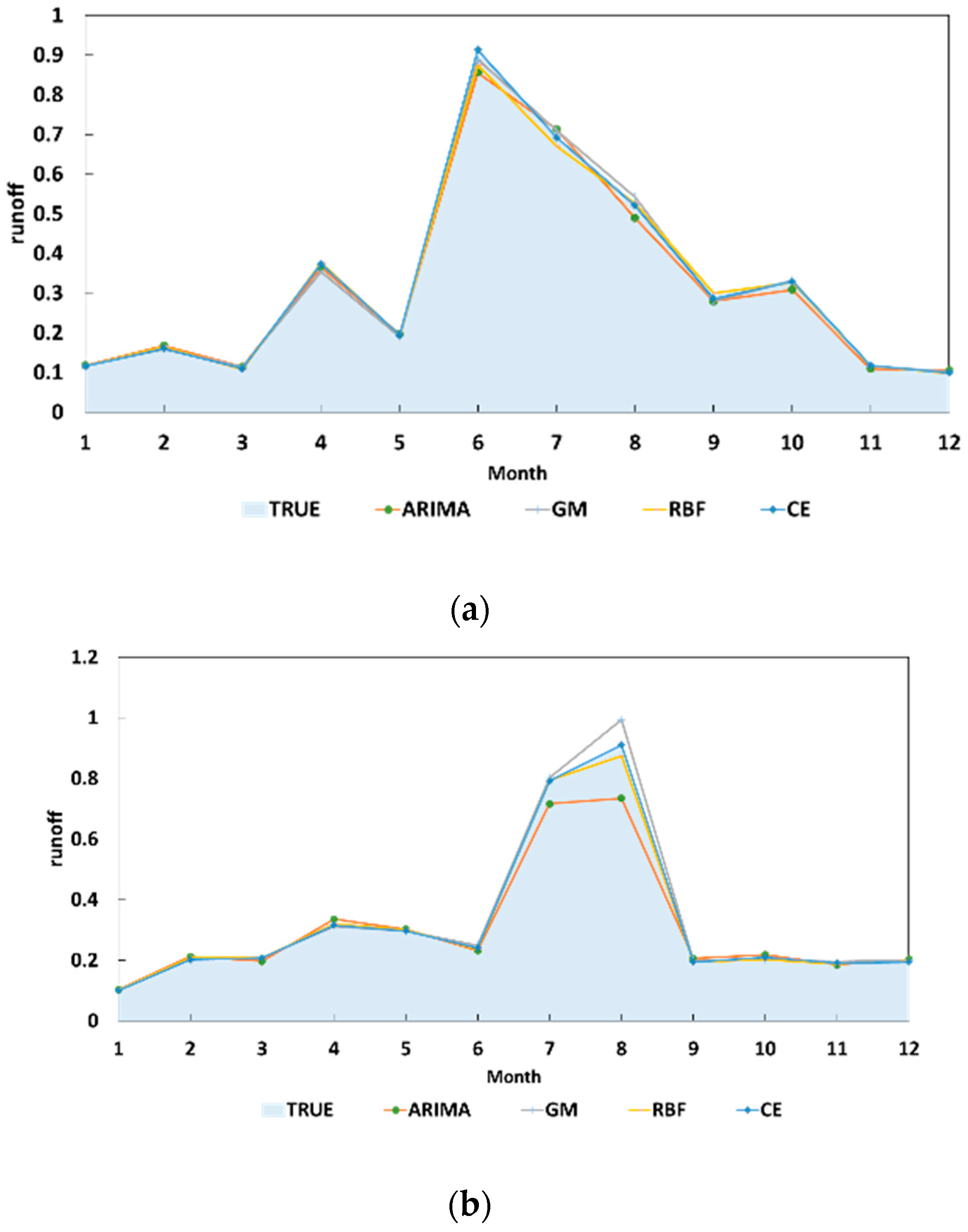
5.1. Comparison of the Results Obtained with a Single Method

The annual forecasting results for 2009–2010 are shown in Figure 4 (the streamflow value has been normalized; see Equation (2)) and the error analysis for these results is shown in

Table 1. Error analysis of the results.

Year	ARIMA		GM		RBF		CE
	MRPE	RMSE	MRPE	RMSE	MRPE	RMSE	MRPE	RMSE
2006	10.95%	6.96%	10.55%	4.79%	10.58%	3.98%	10.53%	3.67%
2007	10.66%	5.77%	9.23%	5.61%	9.07%	4.89%	8.95%	5.01%
2008	9.71%	6.01%	10.12%	5.85%	9.25%	5.28%	9.77%	5.32%
2009	9.89%	5.25%	10.35%	6.08%	7.32%	5.01%	7.24%	4.99%
2010	11.27%	7.38%	11.59%	8.91%	8.56%	7.97%	8.30%	6.67%
Average	10.50%	6.27%	10.37%	6.25%	8.96%	5.43%	8.96%	5.13%

.

Based on Table 1 and Figure 4, we can give the following conclusions: (1) compared with the RMSE for a single method, the combined forecasting method was not optimal for a certain prediction point but the overall error was low compared with GM, ARIMA, and RBF, with reductions of 1.14%, 1.12%, and 0.3%, respectively. The combined forecasting method had higher accuracy; (2) the MRPE index was very high with a single method, e.g., August 2010, and there was a risk of the model failing. The combined forecasting method greatly reduced the MRPE and its predictions had greater stability; and (3) the prediction error was relatively large using a single method (e.g., in 2010) and, thus, the error of the combined forecasts was relatively large, so the accuracy of the single forecasting models affected the accuracy of the combined model.

5.2. Comparison with Other Combined Forecasting Models

In order to demonstrate the improved accuracy of the predictions obtained by the CE combined forecasting model, we performed comparisons with two other methods for combined forecasting, i.e., equal weight combined forecasting (EW) and the regression model (RM). The objective function of the RM model is:

$$\min e_c^2=\min {\displaystyle \sum }_{t=1}^n{\left|{\hat{y}}_c\left(\mathrm{t}\right)-y\left(\mathrm{t}\right)\right|}^2=\min {\displaystyle \sum }_{t=1}^n{\displaystyle \sum }_{i=1}^m{\left({\omega }_i{\hat{y}}_i\left(\mathrm{t}\right)-y\left(\mathrm{t}\right)\right)}^2$$

(26)

i.e., to meet minimize the forecast error of the square in n years, where we set n as 5. The analysis of the predicted results is shown in

Table 2. Error analysis of the results.

Year	EW		RM		CE
	MPE	RMSE	MPE	RMSE	MPE	RMSE
2006	10.76%	3.75%	10.53%	3.71%	10.53%	3.67%
2007	9.23%	5.56%	9.14%	5.34%	8.95%	5.01%
2008	9.74%	5.30%	9.78%	5.29%	9.77%	5.32%
2009	7.55%	5.09%	7.43%	5.25%	7.24%	4.99%
2010	10.07%	7.24%	9.52%	7.08%	8.30%	6.67%
Average	9.47%	5.39%	9.28%	5.33%	8.96%	5.13%

.

The comparison of the predicted results showed that the CE model performed better than the EW and RM models, where it exhibited greater stability. This is because the single method is based on a probability density function and it is the largest single method, although not a simple one. Thus, the predicted results were more suitable for combined forecasting.

5.3. Influence of the Historical Data Length on the Prediction Results

In order to compare the stability of the prediction method, we reduced the length of the historical data, as follows. Case 1: delete the data from 65–75; Case 2: delete the data from 75–85; Case 3: delete the data from 95–05. The results (averages from 06–10) obtained for CE, RM, and RBF are compared in

Table 3. Comparison of the CE, RM, and RBF results.

Case	RBF		RM		CE
	MPE	RMSE	MPE	RMSE	MPE	RMSE
Case 1	9.01%	5.62%	9.31%	5.37%	8.98%	5.14%
Case 2	9.37%	5.71%	9.42%	5.43%	9.11%	5.25%
Case 3	12.94%	7.87%	11.28%	7.01%	10.50%	6.62%

.

The comparison of the predicted results in Table 3 shows the following: (1) the historical data have a great effect on the prediction results, which is stronger closer to the forecasting date. The forecasting accuracy is significantly reduced when the data are missing close to the forecasting date (Case 3); and (2) in all cases, the prediction accuracy of the CE model is highest, which indicates that the anti-disturbance ability of the model is better and its predictions are more stable.

6. Conclusions

Due to the combined effects of climate, natural geography, social development, and human activities, the changes in the streamflow are complex in a basin, with random, grey, and nonlinear characteristics. In this study, we proposed a combined forecasting model based on the CE, where we analyzed the variation in streamflow and the reasonable selection of similar years. The similarity of several single methods was used as basic data in the combined forecasting model, where the weights of the combined methods were determined using the Lagrange function. The results showed that, compared with single forecasting models and other combined forecasting models, the forecasting model based on the CE could improve the accuracy and reliability of streamflow forecasting, as well as guaranteeing the accuracy of the error for a single method, thereby making the forecast results more accurate and reliable. The improved combined forecasting method was very useful for describing the variation in streamflow and it improved the stability of the predictions. These predictions can help agriculture and water conservancy departments to develop reasonable plans for the management of water resources.

In the future, we plan to make the following improvements: (1) we will improve the prediction accuracy of single forecasting methods by considering the time characteristics using data mining as well as the validity of the assessment data; (2) we will identify the factors related to streamflow in a more scientific manner; and (3) the probability density function method will be improved so the relationship between the combined forecasting model function and the single model function is more accurate, with more accurate and reliable weights.

References

1. Zhang, L.X.; Lei, X.Y. Decomposition of time series model in wulasitai River application of annual runoff prediction. J. Water Resour. Water Eng. 2006, 17, 22–24. [Google Scholar]
2. Emili, B.; Alberto, P.; Emilio, S.; Jose, D. Predicting service request in support centers based on nonlinear dynamics ARMA modeling and neural networks. Expert Syst. Appl. 2008, 34, 665–672. [Google Scholar]
3. Li, B.; Yuan, P.; Chang, J. GM (1,1) improved model for predicting annual runoff forecasting. Northeast Water Conserv. Hydroelect. 2006, 24, 28–30. [Google Scholar]
4. Yu, G.R.; Ye, H.; Xie, Z.Q. Projection pursuit auto regression model in predicting runoff of Yangtze River in application. Hohai Univ. J. 2009, 37, 263–266. [Google Scholar]
5. Zhou, H.F.; Li, C. The main stream of the Yellow River Runoff of transient components and frequency analysis and its prediction. Meteor. Sci. 2003, 23, 201–207. [Google Scholar]
6. Qiu, L.; An, K.J.; Wang, W.C. Classification of runoff prediction model based on Markov Bayes. Water Conserv. Sci. Technol. Econ. 2011, 17, 1–4. [Google Scholar]
7. Wang, Q.H.; Qian, X.; Zhang, Y.C. Application of BP neural network in the prediction of runoff and stream reservoir runoff forecast. Environ. Protect. Sci. 2010, 23, 19–23. [Google Scholar]
8. Muhsin, N.; Sinan, U.; Irfan, Y. Side-by-side comparison of horizontal surface flow and free water surface flow constructed wet lands and artificial neural network(ANN)modeling approach. Ecol. Eng. 2009, 35, 1255–1263. [Google Scholar]
9. Yun, W.; Guo, S.L.; Xiong, L.H.; Liu, P.; Liu, D. Daily Runoff Forecasting Model Based on ANN and Data Preprocessing Techniques. Water 2015, 7, 4144–4160. [Google Scholar]
10. Hao, Z.C.; Hao, F.H.; Singh, V.P. A general framework for multivariate multi-index drought prediction based on Multivariate Ensemble Streamflow Prediction (MESP). J. Hydrol. 2016, 539, 1–10. [Google Scholar] [CrossRef]
11. Masselot, P.; Dabo-Niang, S.; Chebana, F.; Ouarda, T.B.M.J. Streamflow forecasting using functional regression. J. Hydrol. 2016, 538, 754–766. [Google Scholar] [CrossRef]
12. Arsenault, R.; Poissant, D.; Brissette, F. Parameter dimensionality reduction of a conceptual model for streamflow prediction in Canadian, snowmelt dominated ungauged basins. Adv. Water Resour. 2015, 85, 27–44. [Google Scholar] [CrossRef]
13. Bates, J.; Granger, C. The combination of forecast. Oper. Res. Quart. 1969, 20, 451–468. [Google Scholar] [CrossRef]
14. Gu, H.Y. Prediction of River Runoff. Master’s Thesis, Northeast Forestry University, Harbin, China, June 2008. [Google Scholar]
15. Fan, Y.; Li, Y. Annual runoff combination forecasting method research and application. North Water Conserv. Hydrol. Power 2006, 24, 23–27. [Google Scholar]
16. Yin, J.X.; Jiang, Y.Z.; Lu, F. Based on combination forecasting model of long-term forecasting of reservoir runoff. People’s Yellow River 2008, 30, 28–32. [Google Scholar]
17. Su, X.H. Study on the Short-Term Load Forecasting Based on Artificial Neural Network. Master’s Thesis, Chongqing University, Chongqing, China, May 2005. [Google Scholar]
18. Singh, V.P. Entropy Theory and Its Applications in Environmental and Water Engineering; John Wiley: New York, NY, USA, 2013; p. 662. [Google Scholar]
19. Marini, G.; De Martino, G.; Fontana, N.; Fiorentino, M.; Singh, V.P. Entropy approach for 2D velocity distribution in open-channel flow. J. Hydraul. Res. 2011, 49, 784–790. [Google Scholar] [CrossRef]
20. Fontana, N.; Marini, G.; De Paola, F. Experimental assessment of a 2-D entropy-based model for velocity distribution in open channel flow. Entropy 2013, 15, 988–998. [Google Scholar] [CrossRef] [Green Version]
21. Li, R.; Liu, H.L.; Lu, Y.; Han, B. A combination method for distribution transformer life prediction based on cross entropy theory. Power Syst. Protect. Control 2014, 42, 97–101. [Google Scholar]
22. Chen, N.; Sha, Q.; Tang, Y.; Oi, Y.; Zhu, L. A Combination Method for Wind Power Predication Based on Cross Entropy Theory. Proc. CSEE 2012, 32, 29–34. [Google Scholar]
23. Liu, J.; Nie, C.X.; Xie, Q. Changes of rainfall runoff relationship and the reasons for the status quo analysis. Anhui Agric. Sci. 2010, 38, 5170–5172. [Google Scholar]
24. Liu, H.W. The Feature Selection Algorithm Based on Information Entropy. Master’s Thesis, Jilin University, Jilin, China, June 2010. [Google Scholar]
25. Box, G.E.; Jenkins, G.M. Time Series Analysis: Forecasting and Control, revised ed.; Holden Day: San Francisco, CA, USA, 1976; pp. 80–145. [Google Scholar]
26. Si, Q. The Gray Prediction Model of Equal Dimension and New Information and the Forecasting Precision—Based on the Analysis and Prediction of the Pension Insurance for Urban Residents of China. Stat. Thinktank 2008, 12, 13–19. (In Chinese) [Google Scholar]
27. Pieter-tjerk, D.B.; Kroese, D.P.; Shie, M.; Rubinstein, R.Y. A Tutorial on the Cross-Entropy Method. Annal. Oper. Res. 2005, 134, 19–67. [Google Scholar]
Figure 1. Monthly streamflow at Wudaogou station during 1965–2010.
Entropy 18 00336 g001
Figure 2. Annual streamflow, annual rainfall, and the ratio of the two curves at Wudaogou station during 1965–2010.
Entropy 18 00336 g002
Figure 3. Flowchart illustrating the algorithm.
Entropy 18 00336 g003
Figure 4. Forecast annual streamflow curve. (a) Annual forecast results in 2009; (b) Annual forecast results in 2010.
Entropy 18 00336 g004