On Multi-Scale Entropy Analysis of Order-Tracking Measurement for Bearing Fault Diagnosis under Variable Speed

Abstract

The research objective in this paper is to investigate the feasibility and effectiveness of utilizing envelope extraction combining the multi-scale entropy (MSE) analysis for identifying different roller bearing faults. The features were extracted from the angle-domain vibration signals that were measured through the hardware-implemented order-tracking technique, so that the characteristics of bearing defects are not affected by the rotating speed. The envelope analysis was employed to the vibration measurements as well as the selected intrinsic mode function (IMF) that was separated by the empirical mode decomposition (EMD) method. By using the coarse-grain process, the entropy of the envelope signals in the different scales was calculated to form the MSE distributions that represent the complexity of the signals. The decision tree was used to distinguish the entropy-related features which reveal the different classes of bearing faults.

1. Introduction

Due to the large system size or the limitations of environmental hazards, it may be difficult to inspect the bearings of rotating machinery directly. Therefore, vibration analysis, which is an indirect approach for system dynamics analysis has been applied to diagnose the bearing faults in rotating machinery for decades. In order to retain the performance and efficiency of machinery, it is essential to identify the bearing deterioration in the early stage, and then take the necessary actions for the system maintenance.

Based on the information theory, it is well-known that the system complexity can be estimated by means of the entropy computation. Since the entropy represents the complexity estimation of the system measurements, different types of entropy definitions, such as the sample entropy [1,2], approximate entropy [1,3], spectral entropy [4], pattern spectrum entropy [5], permutation entropy [6,7], and energy entropy [8], have been utilized to evaluate the regularity or disorderliness of the mechanical and physiological systems. Therefore, such a statistical quantification approach has been employed to diagnose the detriment and malfunction of machinery. In addition, Costa et al. [9,10] indicated that the heartbeat time series of different pathological patients cannot be classified if calculating the sample entropy of the time series in only one temporal-domain scale. Therefore, they proposed the multi-scale entropy (MSE) analysis method to separate the human heartbeat signals of healthy and pathological groups. Based on the concept of MSE analysis, Wu et al. [11] proposed an approach for the diagnosis of ball bearing faults through the MSE analysis as well as the Mahalanobis distance computation. A similar concept was also applied for diagnosing the different faults in high-speed spindle systems [12].

As shown in the previous literature, most studies of the entropy analysis for machine fault diagnostics were achieved based on the operation condition of steady rotating speed. However, some of the rotating systems may operate under the situations of variable rotating speed because of the variation of loads or environmental influence. In such a variable-speed condition, the dynamic features, such as the characteristic frequencies of bearing defects, are strongly governed by the rotating speed. Therefore, it definitely helps to enhance the accuracy of the diagnostics if the influence of variable rotating speed is removed or alleviated. Order-tracking techniques have been utilized to record the vibration signals of rotating machinery in terms of the identical angular displacement instead of the identical sampling time. In such a way, the factor of rotating speed is removed and then the system characteristics can be represented in terms of the orders. Fyfe and Munck [13] utilized the interpolation algorithm to re-construct the signals, such that the measurements seemed to be sampled by means of an identical angular displacement. The computed order-tracking methods were, thus, employed extensively to analyze and diagnose the rotating machineries in order domain [14,15]. Although the computed order-tracking techniques have been broadly utilized to characterize the rotating machinery without the factor of rotating speed, however, such a post-process of software implementation needs the sophisticated interpolation algorithms and may result in imprecise or distorted signals that are reconstructed by the interpolation algorithms. Moreover, the major drawback of the computed order-tracking method is that the information of the shaft rotating speed must be available synchronously while using this kind of technique.

To advance the state-of-art of bearing fault diagnosis in case of variable rotating speed, the hardware-implemented order-tracking technique was utilized in this research to record the precise angular series of vibration. With the identical angular measurement, the influence of the shaft rotating speed upon the fault-related characteristics of the rotary systems can be alleviated and, thus, the variable shaft speed does not affect the features of bearing defects. Since the previous studies have shown that the entropy estimation can represent the disorderliness or complexity of the signal which reflects the different machine faults, the MSE analysis was employed in this research to extract the entropy-related features for bearing defect diagnosis. A bearing test stand consisting of the mechanism of identical angular measurements was performed to illustrate the different types and levels of bearing detriment under the running conditions of variable rotating speed. The bearing defect-related features were extracted to form the feature vectors which contain the MSE distribution among different scales, the cosine values between the MSEs of the normal and faulted bearings, and the sample entropy variation among different scales. A decision tree was employed to verify the performance of intelligent classification among the extracted features. The classification results demonstrated that the proposed approach is capable of diagnosing the different types and levels of bearing detriment accurately. For the purpose of further usage and reference, all of the measurements of the vibration signals and the corresponding shaft rotating speed data that were utilized in this research article are available at the website [16].

2. Vibration Signal Analysis

2.1. Signal Decomposition

The empirical mode decomposition (EMD) proposed by Huang et al. [17] is capable of decomposing the complicated signal into the intrinsic mode functions (IMFs) of different frequency scales, and have been utilized in versatile applications of data analysis, particularly for non-linear and non-stationary signals. Its capability of adaptive time-frequency distribution construction is analogical to the angle-order analysis through the order-tracking techniques for the rotational systems and, hence, can be employed to investigate the bearing vibration in case of variable shaft rotating speed. The vibration signal of identical angular measurement x(k) that was recorded by the hardware-implemented order-tracking technique is decomposed into a number of intrinsic mode functions (IMFs) of different scales (orders) through the EMD method, that is:

$$x(k)={\displaystyle {\sum }_{j=1}^h{c}_j(k)+r_h(k)},$$

(1)

where c_j(k) represents the j-th IMF of the signal x(k), r_h(k) is the signal residue or trend, and k represents the angular index. According to the concept that is analogical to the instantaneous frequencies of IMFs, the decomposed IMF component (Equation (1)) represents the mono-oscillation function, and it exits a unique order at all the instantaneous angles. The IMF must satisfies the following two conditions [17]: (1) The number of extrema and the number of zero-crossings must be either equal or differ at most by one in the whole data set; (2) at any point, the mean value of the envelope defined by the local maxima and the envelope defined by the local minima is zeros. Therefore, it is feasible to compute the physical meaningful orders for the construction of angle-order distributions of the vibration signals that are measured by the order-tracking technique.

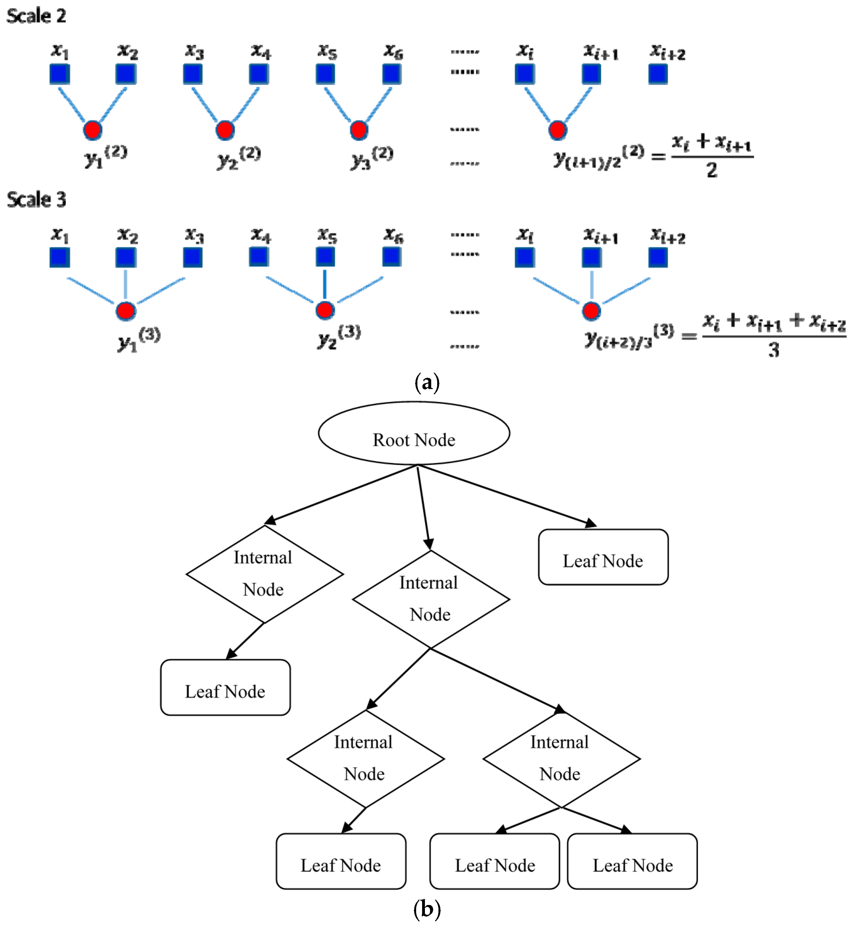
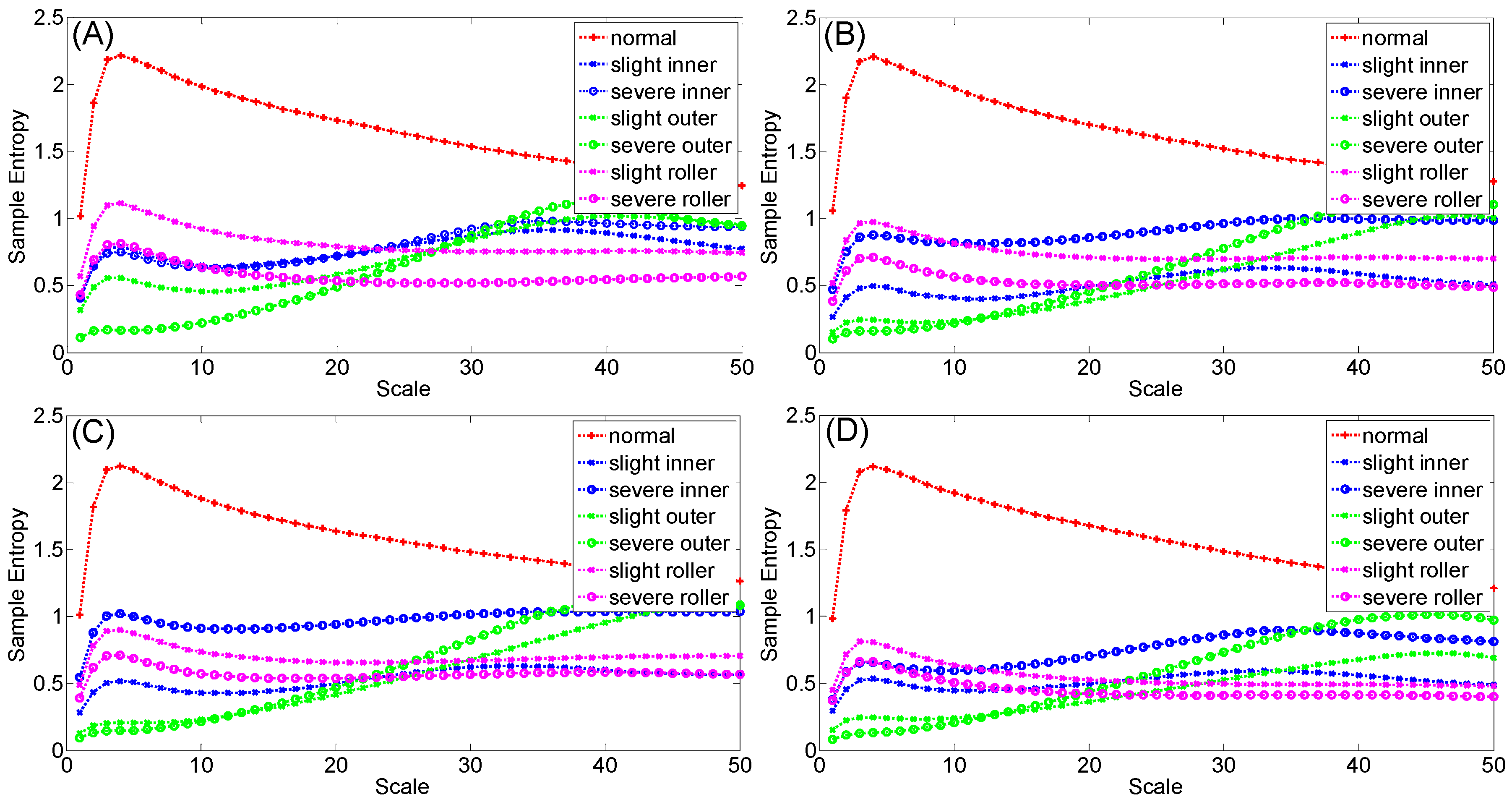
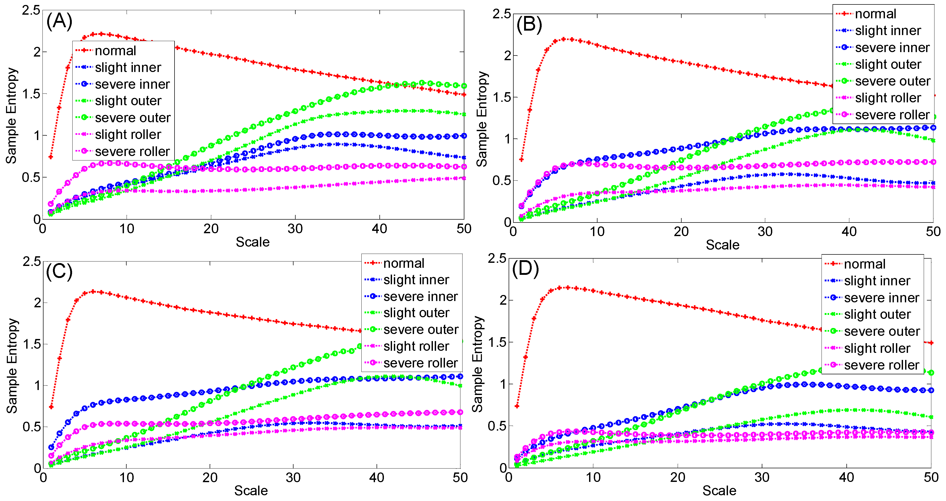
2.2. Computation of Multi-Scale Entropy

In the fields of information theory and thermodynamics, the concept of entropy is conventionally utilized to characterize and estimate the observation data which represent the system dynamical behaviors. Shannon proposed the means to quantify the entropy of the measurements for the characterization of the observation data, and then the method has been extensively applied to measure the complexity or disorderliness of a time series [18]. Suppose a single discrete series S = {x₁, x₂, ..., x_N} has N outcomes in which there exist n classes ({s₁, s₂, ..., s_n}). The entropy of the series S is defined as:

$$En(S)=-{\displaystyle {\sum }_{i=1}^{n}p(s_i)\log (p(s_i))}, s_i\in S,1\le i\le n,$$

(2)

where p(s_i) is the probability density function of the series S, and log represents the natural logarithmic function or logarithmic function to base of 2. Subsequently, Richman and Moorman [1] developed the algorithm to determine the sample entropy (SE) of a series. Let S be the same time series of data length of N as in Equation (2), and m sequential points of the time series be a pattern. Therefore, the pattern space X is defined as [1,6,9]:

$$X=\left[\begin{array}{cccc}{x}_1& x_2& \cdots & x_m\\ x_2& x_3& \cdots & x_{m+1}\\ ⋮\hspace{0.17em}& ⋮& \ddots & ⋮\\ x_{N-m+1}& x_{N-m+2}& \cdots & x_N\end{array}\right].$$

(3)

The mean self-similarity quantity can be formulated as:

$${\phi }_m(r)=\frac{1}{N-m}\frac{1}{N-m+1}{\displaystyle \sum _{i=1}^{N-m}{\displaystyle \sum _{j=1}^{N-m+1}G(d_{ij},r)}},$$

(4)

where G(·) represents the Heaviside function, r is the tolerance and d_ij represents the distance between the i-th and j-th patterns, $d_{ij}={\Vert X_i-X_j\Vert }_{\infty }$. From Equation (4), the mean self-similarity represents the mean value of all the distance measurements between the two sequential patterns X_i and X_j of length m (row vectors of the pattern space X) in terms of the saturation form (Heaviside function). In other words, the self-similarity quantity estimates the repetition degree of sequential pattern of length m. The self-similarity is also calculated for the pattern space of the length of m + 1, and the sample entropy of the series is thus determined as:

$$SEn(m,r)=-\log \frac{{\phi }_{m+1}(r)}{{\phi }_m(r)}.$$

(5)

The concept of entropy in multi-scale was proposed by Costa et al. [9,10]. They indicated that it is difficult to distinguish the inter-beat interval time series of the healthy human beings and the patients with congestive heart fail (CHF) if the sample entropy is examined within only a single temporal-domain scale. In order to resolve this weakness, they proposed the concept of MSE to represent the regularity of the data series in different scales through the coarse-grain process. Their analysis results demonstrated the effectiveness of utilizing the MSE analysis to distinguish the pathological human’s physiological signals. The coarse-grain process is mainly to transform the original data series into different scales. For a given data series, S = {x₁, x₂, ..., x_N}, it is first segmented into several datasets of length τ. By taking the mean values of the segmented data according to the following formula, the new series sets {$y_j^{(\tau )}$} are then obtained:

$$y_j^{(\tau )}=\frac{1}{\tau }{\displaystyle \sum _{i=(j-1)\tau +1}^{j\tau }{x}_i},\hspace{0.17em}\hspace{0.17em}1\le j\le \frac{N}{\tau },$$

(6)

where τ is called the scale factor. Apparently, the coarse-grain process is equivalent to the down-sampling process through using a sliding window of length τ and taking the average of the original signal within the window in the way of non-overlap. Namely, the coarse-grain process is to utilize a moving average filter to remove the high frequency or order components. Figure 1a shows the schematic plot of the coarse-grain process for τ = 2 and τ = 3 [9].

Once the data series is transformed into different scales through the coarse-grain process, the MSE is thus formulated in terms of the different scale τ, that is:

$$MSE(S,\tau ,m,r)=SEn(y^{(\tau )},m,r),$$

(7)

where $y^{(\tau )}=\left\{y_j^{(\tau )}\right\}$ represents the series obtained by the coarse-grain process with the scale τ. The tolerance r is chosen to be fixed in general cases without the variation to the scale τ and, thus, the original signal amplitude does not affect the results of MSE analysis [19].

2.3. Decision Tree Classification

The decision tree is a tree-like model that has been broadly utilized for consequence prediction and data classification. As illustrated in Figure 1b, the structure of the decision tree generally consists of a root node (topmost: input sets of features), leaf nodes (bottommost: class labels), a number of internal nodes, and a number of branches (conjunctions of features). The source set of features are separated into the subsets which are based on the outcome test values of the attributes. The procedure of the decision tree algorithm can be summarized as the following steps:

(1)

The source set of features start training at the root node of the decision tree.

(2)

If the features have the same outcome values of attributes at the same node, then this node is the leaf node and all of the features at the node are classified as the same class label.

(3)

If the features at the node have different outcome values of attributes, then this node belongs to the internal node and the most distinguishable attribute among the features is estimated to discriminate the features. The estimation criteria of this attribute are employed for the decision rule at this node.

(4)

The above steps go through recursively to form the decision tree model.

(5)

The stoppage conditions of the steps include:

(i)

For all nodes in the decision tree, all of the features at the same node have the same outcome values of attributes. Namely, all the nodes go to Step 2.

(ii)

The features at the same node do not consist of attribute to be utilized for further separation.

It is clear that the top node is the best node for classification and the other features at the nodes of the decision trees appear in descending order of importance [20]. The merits of the decision tree classifier includes that the classification rule is simple and less computation effort is required. The algorithms of the decision trees that have been utilized broadly include ID3 [21], C4.5 [22], CHAID [23], CART [24], and QUEST [25]. Due to its flexible capability for continuous and discrete data processing, the C4.5 algorithm [22] was employed in this research to construct the decision tree model for the classification of different bearing defects.

The C4.5 algorithm selects the testing attributes according to the information gains that are determined at each node of the decision tree. Cluster D represents the collection of d sets of data samples. The data samples consist of m class labels, denoted by C_i (i = 1, 2, ..., m) and d_i represents the dataset number of class label C_i. The expectation information of D is computed as:

$$Info(D)=-{\displaystyle \sum _{i=1}^m{p}_i{\log }_2(p_i)},$$

(8)

where p_i represents the probability of the data samples which are classified to C_i, calculated as d_i/d. Suppose the attribute T has v different values {t₁, t₂, ..., t_v}, and thus the cluster D is divided into v subsets {D₁, D₂, ..., D_v}. The entropy of the data cluster D can be formulated as:

$$E(T)=-{\displaystyle \sum _{j=1}^v\frac{d_{1j}+d_{2j}+...+d_{mj}}{d}Info(D)},$$

(9)

where d_kj represents the data set number of the k-th class label having the j-th attribute value.

The information gain of the cluster D with the attribute T is then computed as:

$$Gain(D,T)=Info(D)-E(T).$$

(10)

The algorithm calculates the information gain of each attribute and then selects the attribute of the highest information gain value to be the testing attribute of the node. The training sets of data samples that consist of several known attributes, as well as the known target class labels, are utilized to construct the decision tree model. The data samples whose class labels need to be identified are classified according to the node attributes of the decision tree model.

3. Experiment Verification

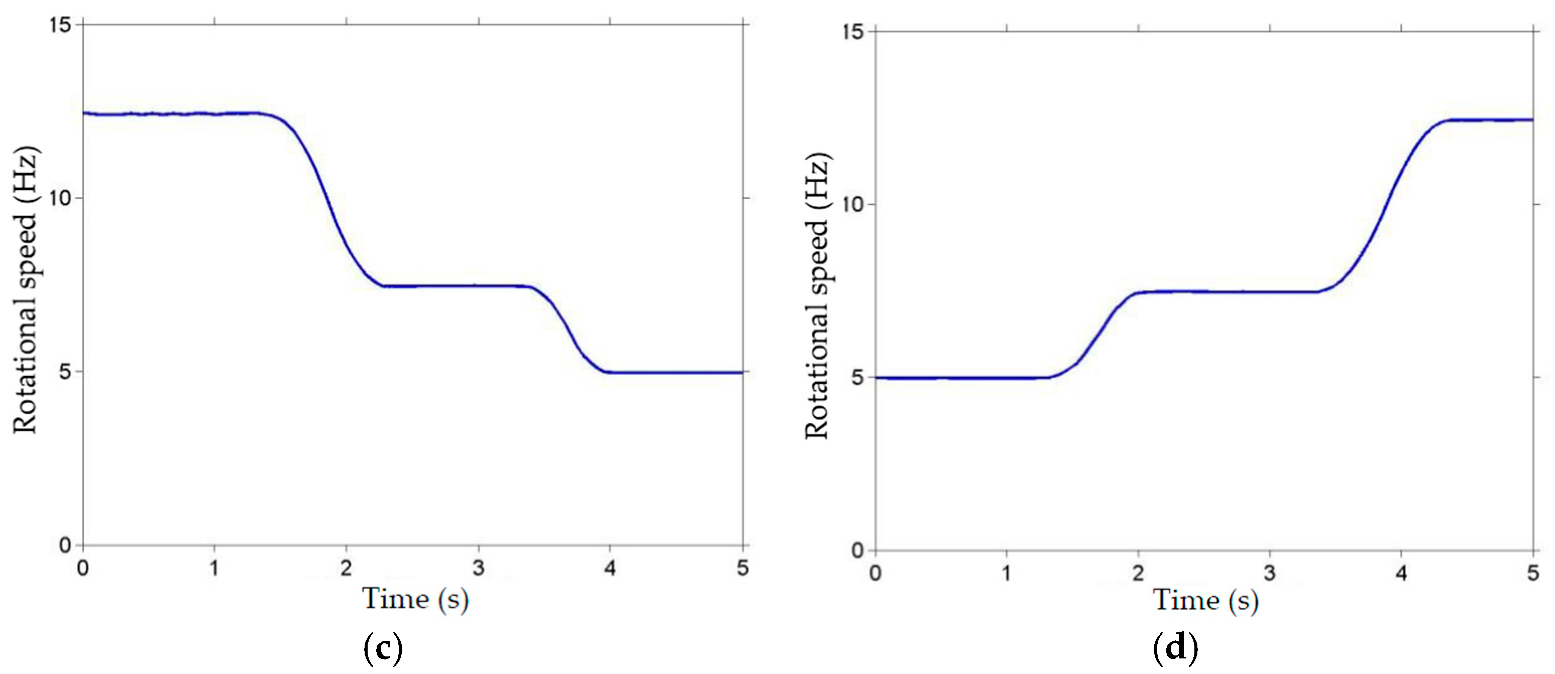
3.1. Experiment Setup

In order to evaluate the diagnostic effectiveness and accuracy of the proposed approach, a bearing testbed was performed to illustrate the different running conditions of defective bearings in this research. The testbed consisted of a main shaft that was supported by a pair of bearing sets. The bearing type used in this research is KOYO N203 (Hongkong NKF Machinery Co., Limited, Hongkong, China), and

Table 1. Characteristics of the bearing in the experiment.

Dimension Specification
Inner diameter (mm)	17	Roller diameter (mm)	6.5
Outer diameter (mm)	40	No. of roller	10
Cage diameter (mm)	28.6
Characteristics			order
Cage rotating order (Oc)			0.39
Roller spin order (Obs)			2.09
Order of roller passing through an outer race point (Obpo)			3.86
Order of a roller point passing through inner and outer race (Orp)			4.17
Order of roller passing through an inner race point (Obpi)			6.14

shows the dimension specifications as well as the associated characteristic orders. The notches of different sizes were first made artificially on the inner race, outer race, and roller of the bearings, respectively, through the electrical discharge machining technique. One of the bearing sets in the test-bed was replaced by the defective bearing to simulate the running conditions with different bearing faults. The driving motor operated following the four different preset profiles of rotating speed (shown in Figure 2), consisting of (A) constant speed; (B) speed-up and speed-down; (C) speed-down; and (D) speed-up, to simulate the running conditions of variable speed. The accelerometer was stuck on the bearing support to measure the vibratory acceleration. The shaft encoder consisting of 600 identical indices per revolution was installed to measure the precise rotating speed. Each index of the shaft encoder can produce a one pulse signal to trigger the data acquisition device (NI 9215) recording the vibratory acceleration signal. With such a mechanism, the vibration signals were captured with identical angle in this hardware-implemented order-tracking configuration and, thus, the characteristics of bearing defects are not related to the rotating speed.

Seven test classes, as shown in

Table 2. Defective bearing class in experiment.

Class	Defect Expression	Notch Dimension
C1	Normal
C2	Slight outer race defect	0.4 mm × 0.3 mm
C3	Severe outer race defect	0.8 mm × 0.3 mm
C4	Slight inner race defect	0.4 mm × 0.3 mm
C5	Severe inner race defect	0.8 mm × 0.3 mm
C6	Slight roller defect	0.1 mm × 0.3 mm
C7	Severe roller defect	0.4 mm × 0.3 mm

were illustrated in this experiment, consisting of the normal case as well as the defective conditions. One hundred datasets of angle-domain vibration signals (25 sets for each shaft rotating speed profile) were acquired to represent the vibration behavior of each experimental class of bearing defect. A total of 700 sets of angle-domain vibration signals, each set containing 21,000 data points, were recorded in this experiment. For the further employment and reference, all the measurements of the vibration signals and the corresponding shaft rotating speed data are available at the website [16].

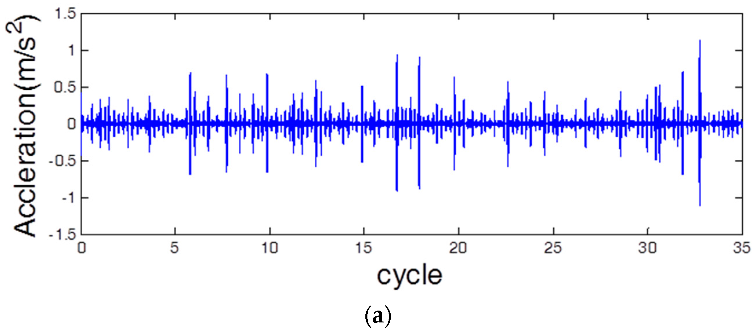
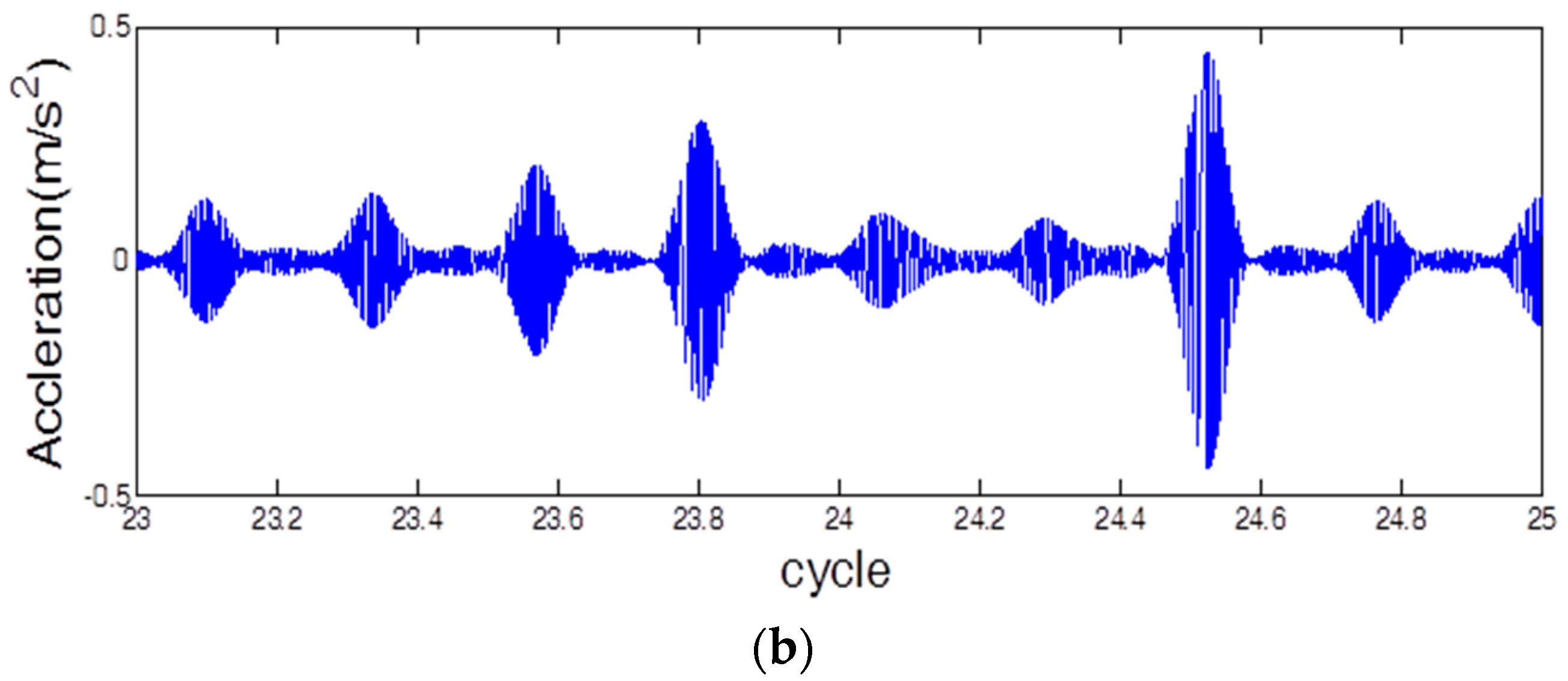
3.2. Vibration Signal Analysis and Processing

All of the recorded vibration signals were separated into a number of IMFs by the EMD method [17]. Since the collected vibration data were identical angular signals, the decomposed IMFs represent the signal components of different orders. In order to ensure that no mode-mixing problem exists in the EMD process, the standard IMF orthogonality index check [17] was also involved in the above signal separation steps. It is also noted that the order values of IMFs do not affect the calculation of MSE, so the angle-order distributions are skipped in this paper. Based on the observation, as well as the physical interpretation, the defective component impacts the other components of bearing cyclically and, thus, the amplitude modulation phenomenon can be observed in the measurements (as illustrated in Figure 3). The cubic spline fitting was then employed to extract the envelope signals of the vibration signals. It is also noted that all the first IMFs of the vibration signals which represents the signal component of the highest order have the apparent amplitude modulation phenomenon (as illustrated in Figure 4). The envelope analysis (cubic spline fitting) was also employed for the first IMFs of all of the vibration signals for comparison purposes.

The MSEs within the first 50 scales were then calculated for all the envelope signals of the original vibration measurements and their first IMF components, respectively. Figure 5 and Figure 6 show the mean MSE quantities of the envelope signals that were extracted from the vibration measurements (testing subset I) and the first IMFs of vibration measurements (testing subset II) under the different defective classes and the corresponding shaft rotation speed. It can be observed in these two figures that the different types of bearing faults present the different distributions of sample entropy among different scales (distinquishability), while the different sample entropy values derive the levels of bearing defects. By observing these two figures and comparing among the subplots (A), (B), (C), and (D) in Figure 5, it is apparent that the rotating speed variation does not affect the distinguishability among the MSE distributions. The MSE quantities of the testing subset II (Figure 6) reveal the distinguished distributions more obviously than the ones of the testing subset I (Figure 5), particularly for the different levels of bearing defects.

3.3. Signal Feature Extraction

In order to provide the decision tree classifier with the representative parameters for bearing defect diagnostics, the fault-related features were extracted through the vibration signal analysis and processing.

The first group of features consists of the MSE values with the first 50 scales, which represent the distinguishability of sample entropy among the different scales. The features in the second group were computed to estimate the difference between the normal and defective classes of bearings. Let A represent the vector of MSE distribution of normal bearing, and B represent the vector of MSE distribution of different defective bearings. The cosine values between the two vectors were calculated as the features of the second group, that is:

$$\cos \theta =\frac{A\cdot B}{\left|A\right|\left|B\right|}$$

(11)

Except for the MSE in the first 50 scales and the cosine values between the MSE distributions, the slope values of sample entropy between the (n + 1)-th and the n-th scales were computed as the third group of features that represent the variations of the MSEs. In this experiment, the features that consisted of the MSE of the first 50 scales, the cosine value as shown in formula (Equation (11)), and the 49 slope values of SEs were selected to be the feature inputs of the root node in the decision tree model.

3.4. Bearing Defect Classification through Decision Tree

The program of the C4.5 decision tree in [26] was utilized in this research. The parameters of the C4.5 algorithm were initially set as the default values. According to model training results, the parameters were tuned slightly, such as TRIAL = 12 and GAINRATIO = 1.12. The details of the parameter explanation can be found in [26]. In this study, the features of the 80 datasets that were randomly selected among the 100 datasets in each class of bearing fault were utilized for training the decision tree model, and then the remaining 20 datasets were used for classification testing. These steps applied to the features of testing subset I and II, respectively, and were repeated through the cross-validation process.

Table 3. Diagnostic result of the decision tree in testing subset I.

Number of Data Set		Classified Fault Class
		C1	C2	C3	C4	C5	C6	C7	Accuracy
True experimental class	C1	100	0	0	0	0	0	0	100%
	C2	0	95	5	0	0	0	0	95%
	C3	0	4	96	0	0	0	0	96%
	C4	0	0	0	97	1	1	1	97%
	C5	1	0	0	3	93	2	0	93%
	C6	0	0	0	2	1	83	14	83%
	C7	0	0	0	0	0	10	90	90%
Overall accuracy									93.4%
Consolidate different levels of roller defects									96.9%

and

Table 4. Diagnostic result of the decision tree in testing subset II.

Number of Data Set		Classified Fault Class
		C1	C2	C3	C4	C5	C6	C7	Accuracy
True experimental class	C1	100	0	0	0	0	0	0	100%
	C2	0	99	1	0	0	0	0	99%
	C3	0	0	100	0	0	0	0	100%
	C4	0	0	0	98	1	0	1	98%
	C5	2	1	0	2	92	0	3	92%
	C6	0	0	0	0	0	86	14	86%
	C7	0	0	2	2	0	13	83	83%
Overall accuracy									94.0%
Consolidate different levels of roller defects									97.9%

show the results of bearing defect diagnostics in the testing subset I and II through the decision tree classification. As shown in the tables, high diagnostic accuracy can be obtained for the classes of C1 to C5, while the diagnostic accuracy of the roller defects is lower. One of the possible reasons is that the skidding phenomenon of the roller may occur during the rotation and, hence, it changes the vibration behavior. The other possible reason is that the features of roller defect in vibration signals are relatively faint and, thus, the features are not distinguishable enough for different levels of roller defects. Conceptually, the EMD process is capable of separating the complicated vibration signals into the useless noise, as well as the information-containing components, and then helps to accurately diagnose the bearing defects. Even though the overall diagnostic accuracy of the testing subset II (94.0%) is slightly higher than that of the testing subset I (93.4%), the diagnostic accuracy of testing subset II (97.9%) will be higher than that of testing subset II (96.9%) if the slight and severe roller defect classes were consolidated into one class of roller defect due to the faint feature of roller defects. In addition, the fast Fourier transform (FFT) was utilized as an alternative method to compare with the proposed MES analysis. The traditional Fourier-based spectra were extracted to be the features of different bearing defects.

Table 5. Diagnostic result with features of Fourier spectra.

Number of Data Set		Classified Fault Class
		C1	C2	C3	C4	C5	C6	C7	Accuracy
True experimental class	C1	100	0	0	0	0	0	0	100%
	C2	0	90	0	2	4	2	2	90%
	C3	0	24	76	0	0	0	0	76%
	C4	0	0	0	100	0	0	0	100%
	C5	0	12	0	16	68	2	2	68%
	C6	0	0	0	0	4	69	27	69%
	C7	0	0	0	0	4	29	67	67%
Overall accuracy									81.4%
Consolidate different levels of roller defects									88.3%

shows the bearing diagnosis result by using the Fourier spectra as the features. It is noted that the conventional Fourier spectrum analysis methods cannot diagnose the bearing faults accurately (88% accuracy in this study) under the conditions of variable speed. Conclusively, the envelope extraction combining the MSE analysis can achieve the bearing fault diagnosis accurately in the case of variable rotation speed.

4. Conclusions

The envelope extraction combining the MSE analysis was employed to diagnose the different types and levels of bearing defects in this research. The hardware-implemented order-tracking technique was utilized to acquire the precise identical angular vibration signals, so that the factor of variable rotating speed can be removed. The complexity of the envelope signals that represents the dynamic characteristics of bearing defects was estimated by the MSE computation. The results of MSE analysis reveal that the feature vectors have obvious distinguishability among the different bearing defects. The decision tree classifier is utilized to identify the features of different bearing defects. The diagnostic results validate the feasibility and effectiveness of the proposed approach for accurately diagnosing the different bearing defects in case of variable rotation speed. More sophisticated signal separation and analysis methods may be needed to process the complicated measurements if the proposed approach is applied for the industrial environment.

References

1. Richman, J.S.; Moorman, J.R. Physiological time-series analysis using approximate entropy and sample entropy. Am. J. Physiol. Heart Circ. Physiol. 2000, 278, H2039–H2049. [Google Scholar] [PubMed]
2. Han, M.H.; Pan, J.L. A fault diagnosis method combined with FEEMD, sample entropy and energy ratio for roller bearings. Measurement 2015, 75, 7–19. [Google Scholar] [CrossRef]
3. Yan, R.; Gao, R.X. Approximate entropy as a diagnosis tool for machine health monitoring. Mech. Syst. Signal Process. 2007, 21, 824–839. [Google Scholar] [CrossRef]
4. Pen, Y.N.; Chen, J.; Li, X.L. Spectral entropy: A complementary index for rolling element bearing performance degradation assessment. Proc. Inst. Mech. Eng. Part C J. Mech. Eng. Sci. 2009, 223, 1223–1231. [Google Scholar] [CrossRef]
5. Hao, R.; Peng, Z.; Feng, Z.; Chu, F. Application of support vector machine based on pattern spectrum entropy in fault diagnostics of rolling element bearings. Meas. Sci. Technol. 2011, 22. [Google Scholar] [CrossRef]
6. Wu, S.D.; Wu, P.H.; Wu, C.W.; Ding, J.J.; Wang, C.C. Bearing fault diagnosis based on multiscale permutation entropy and support vector machine. Entropy 2012, 14, 1343–1356. [Google Scholar] [CrossRef]
7. Shi, Z.L.; Song, W.Q.; Taheri, S. Improved LMD, Permutation Entropy and Optimized K-Means to Fault Diagnosis for Roller Bearings. Entropy 2016, 18, 70. [Google Scholar] [CrossRef]
8. Lei, Y.G.; Zuo, M.J.; He, Z.J.; Zi, Y.Y. A multidimensional hybrid intelligent method for gear fault diagnosis. Expert Syst. Appl. 2010, 37, 1419–1430. [Google Scholar] [CrossRef]
9. Costa, M.; Goldberger, A.L.; Peng, C.K. Multiscale entropy analysis of complex physiologic time series. Phys. Rev. Lett. 2002, 89, 068102. [Google Scholar] [CrossRef] [PubMed]
10. Costa, M.; Goldberger, A.L.; Peng, C.K. Multiscale entropy analysis of biological signals. Phys. Rev. E 2005, 71, 021906. [Google Scholar] [CrossRef] [PubMed]
11. Wu, S.D.; Wu, C.W.; Wu, T.Y.; Wang, C.C. Multi-scale analysis based ball bearing defect diagnostics using Mahalanobis distance and support vector machine. Entropy 2013, 15, 416–433. [Google Scholar] [CrossRef]
12. Hsieh, N.K.; Lin, W.Y.; Young, H.T. High-speed spindle fault diagnosis with the empirical mode decomposition and multiscale entropy method. Entropy 2015, 17, 2170–2183. [Google Scholar] [CrossRef]
13. Fyfe, K.R.; Munck, E.D.S. Analysis of computed order tracking. Mech. Syst. Signal Process. 1997, 11, 187–205. [Google Scholar] [CrossRef]
14. Bai, M.R.; Huang, J.; Hong, M.; Su, F. Fault diagnosis of rotating machinery using an intelligent order tracking system. J. Sound Vib. 2005, 280, 699–718. [Google Scholar] [CrossRef]
15. Wu, J.D.; Huang, C.W.; Chen, J.C. An order-tracking technique for the diagnosis of faults in rotating machineries using a variable step-size affine projection algorithm. NDT E Int. 2005, 38, 119–127. [Google Scholar] [CrossRef]
16. Vibration Measurements for Bearing Defect Diagnosis through Hardware-Implemented Order-Tracking Technique. Available online: http://web.nchu.edu.tw/~tianyauwu/data/bearing/identical_theta/web_data_expression.htm (accessed on 9 August 2016).
17. Huang, N.E.; Shen, Z.; Long, S.R.; Wu, M.C.; Shih, H.H.; Zheng, Q.; Yen, N.-C.; Tung, C.C.; Liu, H.H. The empirical mode decomposition and the Hilbert spectrum for nonlinear and non-stationary time series analysis. Proc. R. Soc. Lond. A 1998, 454, 903–995. [Google Scholar] [CrossRef]
18. Shannon, C.E. A mathematical theory of communication. Bell Syst. Tech. J. 1948, 27, 379–423, 623–656. [Google Scholar] [CrossRef]
19. Costa, M.; Peng, C.K.; Goldberger, A.L.; Hausdorff, J.M. Multiscale entropy analysis of human gait dynamics. Physica A 2003, 330, 53–60. [Google Scholar] [CrossRef]
20. Saravanan, N.; Ramachandran, K.I. Fault diagnosis of spur bevel gear box using discrete wavelet features and Decision Tree classification. Expert Syst. Appl. 2009, 36, 9564–9573. [Google Scholar] [CrossRef]
21. Jin, C.; Li, F.; Li, Y. A generalized fuzzy ID3 algorithm using generalized information entropy. Knowl. Based Syst. 2014, 64, 13–21. [Google Scholar] [CrossRef]
22. Quinlan, J.R. Improved use of continuous attributes in C4.5. J. Artif. Intell. Res. 1996, 4, 77–90. [Google Scholar]
23. Althuwaynee, O.F.; Pradhan, B.; Lee, S. A novel integrated model for assessing landslide susceptibility mapping using CHAID and AHP pair-wise comparison. Int. J. Remote Sens. 2016, 37, 1190–1209. [Google Scholar] [CrossRef]
24. Wickramarachchi, D.C.; Robertson, B.L.; Reale, M.; Price, C.J.; Brown, J. HHCART: An oblique decision tree. Comput. Stat. Data Anal. 2016, 96, 12–23. [Google Scholar] [CrossRef]
25. Chou, J.S. Comparison of multilabel classification models to forecast project dispute resolutions. Expert Syst. Appl. 2012, 39, 10202–10211. [Google Scholar] [CrossRef]
26. Quinlan, J.R. C4.5: Programs for Machine Learning; Morgan Kaufmann Publishers: San Mateo, CA, USA, 1993. [Google Scholar]
Figure 1. Schematic plot of (a) coarse-grain process for τ = 2 and τ = 3 [9] and (b) decision tree.
Entropy 18 00292 g001
Figure 2. Different rotating speed profiles. (a) Constant speed; (b) speed-up and speed-down; (c) speed-down; and (d) speed-up.
Entropy 18 00292 g002aEntropy 18 00292 g002b
Figure 3. Original vibration signals of class C2 under rotation speed profile. (a) Constant speed; (b) speed-up and speed-down; (c) speed-down; and (d) speed-up.
Entropy 18 00292 g003
Figure 4. The first IMF of vibration measurement in class C2 and its zoom-in plot. (a) Original measurement; (b) zoom-in of original measurement.
Entropy 18 00292 g004aEntropy 18 00292 g004b
Figure 5. Mean MSE quantities of envelope signals in testing subset (I) under different defective classes and shaft rotation speed profiles. (A) Constant speed; (B) speed-up and speed-down; (C) speed-down; and (D) speed-up.
Entropy 18 00292 g005
Figure 6. Mean MSE quantities of envelope signals in testing subset (II) under different defective classes and shaft rotation speed profile. (A) Constant speed; (B) speed-up and speed-down; (C) speed-down; and (D) speed-up.
Entropy 18 00292 g006