Normalized Minimum Error Entropy Algorithm with Recursive Power Estimation

Abstract

The minimum error entropy (MEE) algorithm is known to be superior in signal processing applications under impulsive noise. In this paper, based on the analysis of behavior of the optimum weight and the properties of robustness against impulsive noise, a normalized version of the MEE algorithm is proposed. The step size of the MEE algorithm is normalized with the power of input entropy that is estimated recursively for reducing its computational complexity. The proposed algorithm yields lower minimum MSE (mean squared error) and faster convergence speed simultaneously than the original MEE algorithm does in the equalization simulation. On the condition of the same convergence speed, its performance enhancement in steady state MSE is above 3 dB.

1. Introduction

Wired or wireless communication channels are under multipath fading as well as impulsive noise from various sources [1,2]. The impulsive noise can cause large instantaneous errors and system failure so that enhanced signal processing algorithms for coping with such obstacles are needed. Most algorithms are designed based on the mean squared error (MSE) criterion, but it often fails in impulsive noise environments [3].One of the cost functions based on information theoretic learning (ITL), minimum error entropy (MEE) has been developed by Erdogmus [4]. As a nonlinear version of MEE, the decision feedback MEE (DF-MEE) algorithm has been known to yield superior performance under severe channel distortions and impulsive noise environments [5]. It also has been shown for shallow underwater communication channels that the DF-MEE algorithm has not only robustness against impulsive noise and severe multipath fading but can also be more improved by some modification of the kernel size [6].

One of the problems of the MEE algorithm is its heavy computational complexity caused by the computation of double summations for the gradient estimation of MEE algorithm at each iteration time. In the work conducted by [7], a computation reducing method by the recursive gradient estimation of the DF-MEE has been proposed for practical implementation. Though those practical difficulties have been removed through the recursive method, theoretic analysis in depth on its optimum solutions and their behavior has not been carried out yet for further enhancement of the algorithm.

In this paper, based on the analysis of behavior of optimum weight and some factors on mitigation of influence from large errors due to impulsive noise, we propose to employ a time-varying step size through normalization by the input power that is recursively estimated for effectiveness in computational complexity. The performance comparison with MEE will be discussed and experimented through simulation in equalization as well as in system identification problems with impulsive noise that can be encountered in experiments investigating physical phenomenon [8].

2. MSE Criterion and Related Algorithms

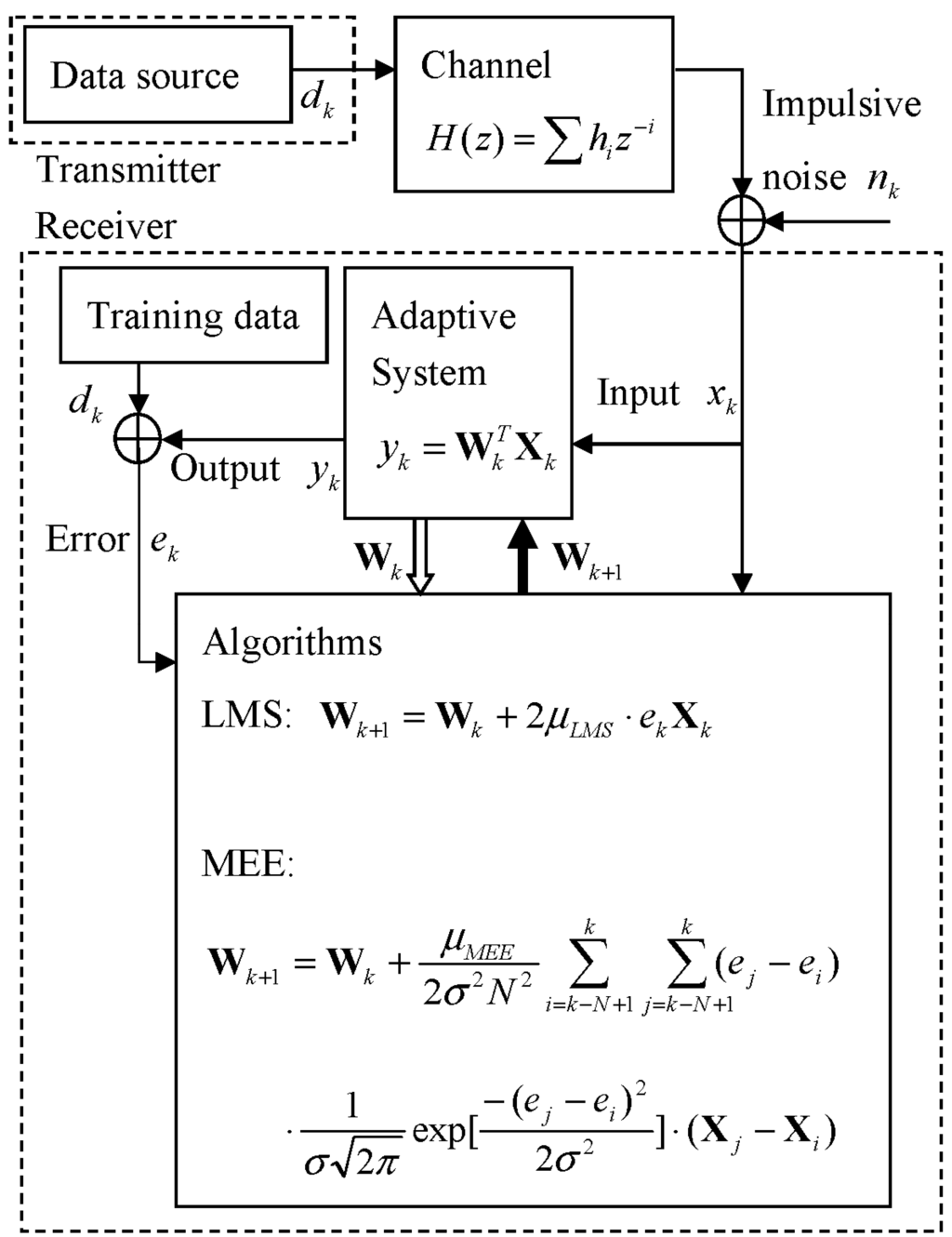
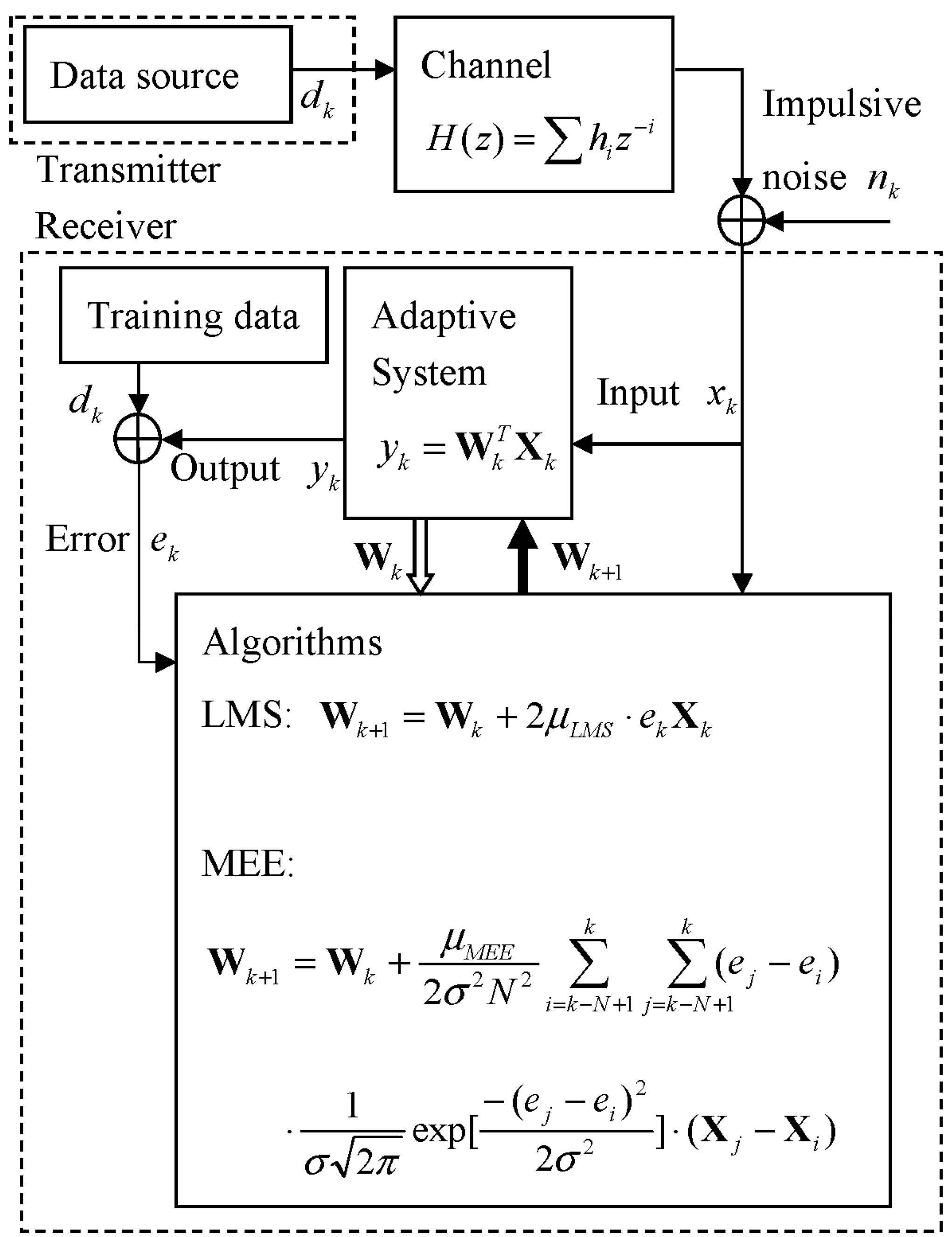
The overall communication system model for this work is described in Figure 1. The transmitter sends a symbol $d_k$ at time k through the multipath channel described in z-transform, $H(z)={\displaystyle \sum h_i}{z}^{-i}$, and then impulsive noise $n_k$ is added to the channel output to become the received signal $x_k$ so that the adaptive system input $x_k$ contains noise $n_k$ and intersymbol interference (ISI) caused by the channel’s multipath [9].

Figure 1. Overall communication system model.

$$x_k={\displaystyle \sum h_i}{d}_{k-i}+n_k.$$

(1)

With the input $X_k={[x_k,x_{k-1},\dots ,x_{k-j},\dots ,x_{k-L+1}]}^T$ and weight $W_k={[w_{0,k},w_{1,k},\mathrm{..},w_{j,k},\dots ,w_{L-1,k}]}^T$ of the tapped delay line (TDL) equalizer, the output $y_k$ and the error $e_k$ become

$$y_k=W_k^T{X}_k,$$

(2)

$$e_k=d_k-y_k=d_k-W_k^T{X}_k.$$

(3)

With the current weight $W_k$, a set of error samples and a set of input samples, the adaptive algorithms designed according to their own criteria such as MSE or MEE produce updated weight $W_{k+1}$ with which the adaptive system makes the next output $y_{k+1}$.

Taking statistical average $E[\cdot ]$ to the error power ${e_k}^2$, the MSE criterion is defined as $E[{e_k}^2]$. For practical reasons, instantaneous error power $e_k^2$ can be used and the LMS (least mean square) algorithm has been developed based on minimization of $e_k^2$ [9].The minimization of $e_k^2$ can be carried out by the steepest descent method utilizing the gradient of $e_k^2$ as

$$\frac{\partial e_k^2}{\partial W}=-2e_k{X}_k.$$

(4)

With Equation (4) and the step size ${\mu }_{LMS}$, the well-known LMS algorithm is presented as

$$W_{k+1}=W_k-{\mu }_{LMS}\cdot \frac{\partial e_k^2}{\partial W}=W_k+2{\mu }_{LMS}\cdot e_k{X}_k.$$

(5)

By letting the gradient $\frac{\partial e_k^2}{\partial W}$ be zero, we have the optimum condition of the LMS as

$$e_k{X}_k=0.$$

(6)

Taking statistical average $E[\cdot ]$ to Equation (6) leads us to the optimum condition of the MSE criterion as

$$E[e_k{X}_k]=0.$$

(7)

Inserting (3) into (6), we get the optimum weight of the LMS algorithm, $W_{LMS}^{opt}$ as

$$W_{LMS}^{opt}={\left(X_k{X}_k^T\right)}^{-1}{d}_k{X}_k.$$

(8)

The optimum weight $W_{LMS}^{opt}$ in (8)might be expected to get wildly shaky in impulsive noise situations since it has no protection measures from such impulses existing in the input vector $X_k$.

When the effect of fluctuations in the input power levels is considered, the fact that the step size ${\mu }_{LMS}$ of the LMS algorithm should be inversely proportional to the power of the input signal $X_k$ leads to the normalized LMS algorithm (NLMS) where its step size is normalized by the squared norm of the input vector ${\Vert X_k\Vert }^2$, that is, ${\mu }_{NLMS}/{\Vert X_k\Vert }^2$ [9]. One of the principal characteristics of the NLMS algorithm is that the parameter ${\mu }_{NLMS}$ is dimensionless, whereas ${\mu }_{LMS}$ has the dimensioning of inverse power as mentioned above. Therefore, we may view that the NLMS algorithm has an input power-dependent adaptation step size, so that the effect of fluctuations in the power levels of the input signal is compensated at the adaptation level. When we assume that in the steady state $e_k$ and $X_k$ are independent, the input vector $X_k$ can be viewed as being normalized by its squared norm ${\Vert X_k\Vert }^2$ in the NLMS algorithm as $W_{k+1}=W_k+2{\mu }_{NLMS}\cdot e_k\cdot X_k/{\Vert X_k\Vert }^2$.

Unlike the LMS or NLMS, the MEE algorithm based on the error entropy criterion is known for its robustness against impulsive noise [6]. In the following section, the MEE algorithm will be analyzed with respect to its weight behavior under impulsive noise environments.

3. MEE Algorithm and Magnitude Controlled Input Entropy

The MSE criterion is effective under the assumptions of linearity and Gaussianity since it uses only second order statistics of the error signal. When the noise is impulsive, a criterion considering all the higher order statistics of the error signal would be more appropriate.

Error entropy as a scalar quantity provides a measure of the average information contained in a given error distribution. With N samples (sample size N) of error samples $\{e_k,e_{k-1},\dots ,e_{k-N+1}\}$ the distribution function of error, $f_E(e)$ can be constructed based on Kernel density estimation as in Equation (9) [10].

$$f_E(e)=\frac{1}{N}{\displaystyle \sum _{i=k-N+}^k{G}_{\sigma }(e-e_i)}=\frac{1}{N}{\displaystyle \sum _{i=k-N+1}^k\frac{1}{\sigma \sqrt{2\pi }}\text{exp}[\frac{-{(e-e_i)}^2}{2{\sigma }^2}]}.$$

(9)

Since the Shannon’s entropy in [9] is hard to estimate and to minimize due to the integral of the logarithm of a given distribution function, Renyi’s quadratic error entropy $H(e)$ has been effectively used in ITL methods as described in (10).

$$H(e)=-\text{log}({\displaystyle \int f_E{(e)}^{2}de}).$$

(10)

When error entropy $H(e)$ in (10) is minimized, the error distribution $f_E(e)$ of an adaptive system is contracted and all higher order moments are minimized [4].

Inserting (9) into (10) leads to the following $H(e)$ that can be interpreted as interactions among pairs of error samples where error samples act as physical particles.

$$H(e)=-\text{log}\left[\frac{1}{N^2}{\displaystyle \sum _{i=k-N+1}^k{\displaystyle \sum _{j=k-N+1}^k{G}_{\sigma \sqrt{2}}(e_j-e_i)}}\right].$$

(11)

Since the Gaussian kernel $G_{\sigma \sqrt{2}}(e_j-e_i)$ is always positive and is an exponential decay function with the distance square, the Gaussian kernel may be considered to create a potential field. The sum of all pairs of interactions in the argument of log [.] in (11) is called information potential $I{P}_e$ [4].

$$I{P}_e=\frac{1}{N^2}{\displaystyle \sum _{i=k-N+1}^k{\displaystyle \sum _{j=k-N+1}^k{G}_{\sigma \sqrt{2}}(e_j-e_i)}}.$$

(12)

Then, minimization of error entropy is equivalent to maximization of $I{P}_e$. For the maximization of $I{P}_e$, the gradient of (12) becomes

$$\frac{\partial I{P}_e}{\partial W}=\frac{1}{2{\sigma }^2{N}^2}{\displaystyle \sum _{i=k-N+1}^k{\displaystyle \sum _{j=k-N+1}^k(e_j-e_i)}}\cdot G_{\sigma \sqrt{2}}(e_j-e_i)\cdot (X_j-X_i).$$

(13)

At the optimum state ($\raisebox{1ex}{$\partial I{P}_e$}\!\left/ \!\raisebox{-1ex}{$\partial W$}\right.=0$), we have

$${\displaystyle \sum _{i=k-N+1}^k{\displaystyle \sum _{j=k-N+1}^k(e_j-e_i)}}\cdot G_{\sigma \sqrt{2}}(e_j-e_i)\cdot (X_j-X_i).$$

(14)

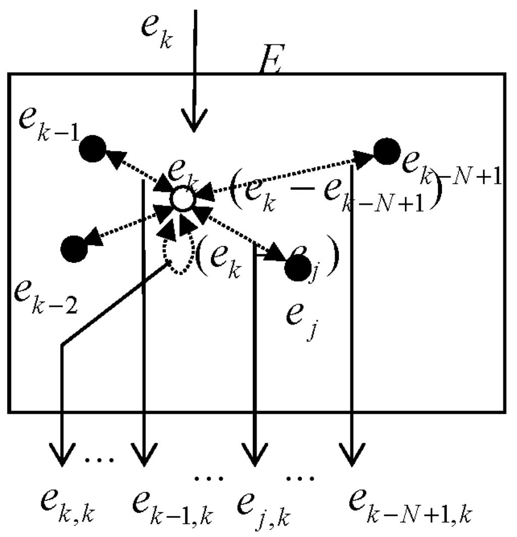
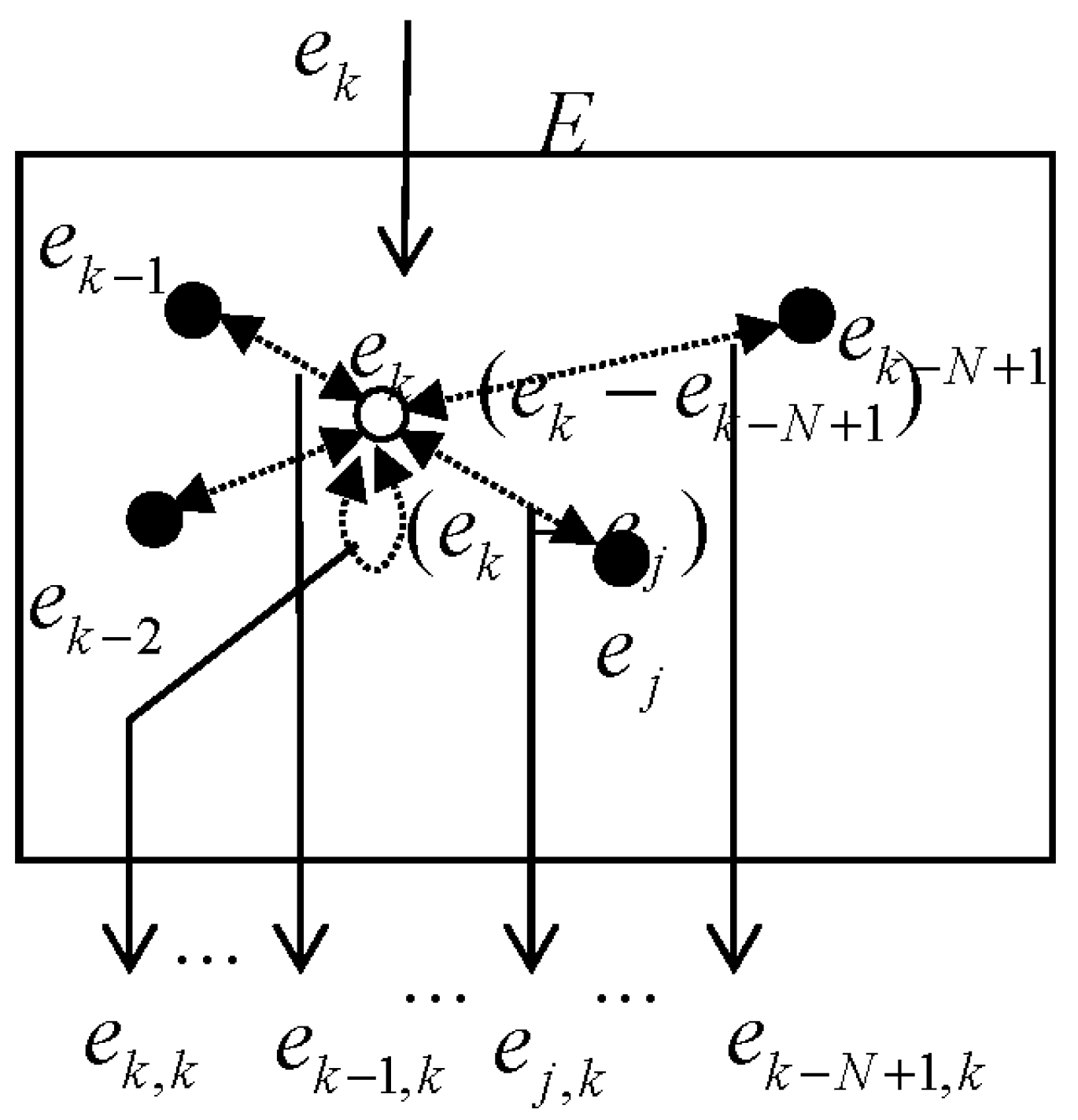
Since the term $(e_j-e_k)$ implies how far the current error $e_k$ is located from each error sample $e_j$, we may define the error pair $(e_j-e_k)$ as $e_{j,k}$ which is generated from the error space $E$ at each iteration time as in Figure 2. The term $e_{j,k}$ can be considered to contain information of the extent of spread of error samples. Considering that entropy is a measure of how evenly energy is distributed or the range of positions of components of a system, we will refer to this information as error entropy (EE) in this paper for convenience.

Figure 2. Error space E and error entropy samples generated from error pairs.

Similarly, the term $(X_j-X_k)$ indicates the distance between the current input vector $X_k$ and another input vector $X_j$ in the input vector space. Therefore, with the following definition, we can say that $X_{j,k}$ contains the information of the extent of spread of input vectors, that is, input entropy (IE). Likewise, we will refer to $X_{j,k}$ as an IE vector in this paper.

$$X_{j,k}=(X_j-X_k).$$

(15)

Then, with the EE sample $e_{j,k}$ and IE vector $X_{j,k}$ Equation (14) can be rewritten as

$$\frac{1}{N}{\displaystyle \sum _{i=k-N+1}^k[{\displaystyle \sum _{j=k-N+1}^k{e}_{j,i}\cdot G_{\sigma \sqrt{2}}(e_{j,i})X_{j,i}]}}=0.$$

(16)

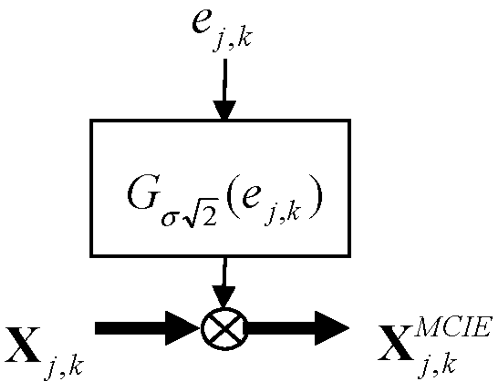
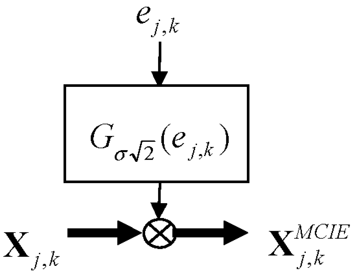
If we consider the sample-averaged operation $\frac{1}{N}{\displaystyle \sum _{i=k-N+1}^k(\cdot )}$ in (16) can be replaced with the statistical average $E[\cdot ]$ or vice versa for practical reasons, the comparison between (16) and the optimum condition of the MSE criterion $E[e_k{X}_k]=0$ in (7) provides insight that $e_k$ of the MSE criterion can correspond to EE sample $e_{j,k}$, and $X_k$ of MSE criterion can be related to $G_{\sigma \sqrt{2}}(e_{j,k})X_{j,k}$ as a kind of modified input entropy vector. We also see that the term $G_{\sigma \sqrt{2}}(e_{j,k})X_{j,k}$ in (16) implies that the magnitude of $X_{j,k}$ is controlled by $G_{\sigma \sqrt{2}}(e_{j,k})$. At the occurrence of a strong impulse in $n_k$,$e_k$ can be located far away from $e_j$ so that the EE sample $e_{j,k}$ has a very large value. Then, the Gaussian function output $G_{\sigma \sqrt{2}}(e_{j,k})$ becomes a very small value since its exponential is a decay function of $e_{j,k}^2$. In turn, the value of the IE vector $X_{j,k}$ is reduced by the multiplication of $G_{\sigma \sqrt{2}}(e_{j,k})$. In this regard, it is appropriate that the term $G_{\sigma \sqrt{2}}(e_{j,k})X_{j,k}$ in (16)is interpreted as a magnitude-controlled version of ... Defining $X_{j,k}^{MCIE}$ as a magnitude controlled input entropy (MCIE) in (17), this process can be described as in Figure 3.

$$X_{j,k}^{MCIE}=G_{\sigma \sqrt{2}}(e_{j,k})X_{j,k}.$$

(17)

Figure 3. Magnitude controller for IE.

In an element expression,

$$x_{j,k}^{MCIE}=G_{\sigma \sqrt{2}}(e_{j,k})x_{j,k}=G_{\sigma \sqrt{2}}(e_{j,k})(x_j-x_k).$$

(18)

With $X_{j,k}^{MCIE}$, the MEE algorithm becomes

$$W_{k+1}=W_k+\frac{{\mu }_{MEE}}{2{\sigma }^2{N}^2}{\displaystyle \sum _{i=k-N+1}^k{\displaystyle \sum _{j=k-N+1}^k{e}_{j,i}}}{X}_{j,i}^{MCIE}.$$

(19)

The optimum condition in (16) can be rewritten as

$$E[{\displaystyle \sum _{j=k-N+1}^k{e}_{j,k}}\cdot X_{j,k}^{MCIE}]=0.$$

(20)

We may observe that the MEE algorithm in (20) is very similar to (7) in the aspect of the error and input terms. One different part is that the MEE algorithm consists of summations of error entropy samples and input entropy vectors, while the LMS just has an error sample and an input vector.

On the other hand, it can be noticed that MCIE $X_{j,i}^{MCIE}$ can keep the algorithm stable even at the occurrences of large error entropy that occurs mostly when the input is contaminated by impulse noise. The summation process over $e_{j,i}{X}_{j,i}^{MCIE}$ can also mitigate the influence of impulses, but it does not contribute much to deterring the influence of large errors since even an impulse can dominate the averaging (summation) operation.

4. Recursive Power Estimation of MCIE

The fixed step size of the MEE algorithm may make the MEE require an understanding of the statistics of the input entropy prior to the adaptive filtering operation. This makes it hard in practice to choose an appropriate step size ${\mu }_{MEE}$ that controls its learning speed and stability.

Like the approach of the normalized LMS that solves this kind of problem through normalization by the summed power of the current input samples as in [9,11], we propose heuristically to normalize the step size by the summed power of the current MCIE element in (18) as

$${\mu }_{NMEE}=\frac{\mu }{{\displaystyle \sum _{j=k-N+1}^k{\left|x_{j,k}^{MCIE}\right|}^2}}.$$

(21)

Considering the fact that impulses can defeat the average operation as explained in Section 3, we can notice that the denominator may become large in an incident with impulsive noise; in turn, ${\mu }_{NMEE}$ becomes a very small value, so that it may induce a very slow convergence. To avoid this kind of situation, we may adopt a sliding window as

$${\mu }_{NMEE}=\frac{\mu }{\frac{1}{N}{\displaystyle \sum _{i=k-N+1}^k{\displaystyle \sum _{j=k-N+1}^k{\left|x_{j,i}^{MCIE}\right|}^2}}}.$$

(22)

However, this approach places a heavier computational complexity on the MEE algorithm. For reducing the burdensome computations, we need to track the power recursively using a single-pole low-pass filter, i.e.,

$$P(k)=\beta P(k-1)+(1-\beta ){\displaystyle \sum _{j=k-N+1}^k{\left|x_{j,k}^{MCIE}\right|}^2},$$

(23)

where β $(0<\beta <1)$ controls the bandwidth and time constant of the system whose transfer function $T(z)$ with its input ${\displaystyle \sum _{j=k-N+1}^k{\left|x_{j,k}^{MCIE}\right|}^2}$ is given by

$$T(z)=(1-\beta )\frac{z}{z-\beta }.$$

(24)

Then, the resulting algorithm that we will refer to in this paper as normalized MEE (NMEE) becomes

$$W_{k+1}=W_k+\frac{\mu }{P(k)2{\sigma }^2{N}^2}{\displaystyle \sum _{i=k-N+1}^k{\displaystyle \sum _{j=k-N+1}^k{e}_{j,i}}}{X}_{j,i}^{MCIE}.$$

(25)

On the other hand, the NLMS in (19) has been developed based on the principle of minimum disturbance that states the tap weight change of an adaptive filter from one iteration to the next, that is, the squared Euclidean norm (SEN) of the change in the tap-weight vector, ${\Vert W_{k+1}-W_k\Vert }^2$ should be minimal [9]. From that perspective, the effectiveness of the proposed NMEE algorithm can be analyzed based on the disturbance, SEN, at around the optimum state as

$$SEN={\Vert W_{k+1}-W_k\Vert }^2.$$

(26)

For the existing MEE algorithm of (19),

$$\begin{array}{c}SE{N}_{MEE}={\left(\frac{{\mu }_{MEE}}{2{\sigma }^2{N}^2}\right)}^2{\Vert {\displaystyle \sum _{i=k-N+1}^k{\displaystyle \sum _{j=k-N+1}^k{e}_{j,i}}}{X}_{j,i}^{MCIE}\Vert }^2\\ ={\left(\frac{1}{2{\sigma }^2{N}^2}\right)}^2{{\mu }_{MEE}}^2{\displaystyle \sum _{i=k-N+1}^k{\displaystyle \sum _{j=k-N+1}^k}}{\displaystyle \sum _{l=k-N+1}^k{\displaystyle \sum _{m=k-N+1}^k{e}_{j,i}}}{e}_{m,l}{X}_{j,i}^{MCIET}{X}_{m,l}^{MCIE}.\end{array}$$

(27)

For the proposed NMEE algorithm,

$$SE{N}_{NMEE}={\left(\frac{\mu }{2{\sigma }^2{N}^{2}P(k)}\right)}^2{\Vert {\displaystyle \sum _{i=k-N+1}^k{\displaystyle \sum _{j=k-N+1}^k{e}_{j,i}}}{X}_{j,i}^{MCIE}\Vert }^2.$$

(28)

Then

$$SE{N}_{NMEE}={\left(\frac{1}{2{\sigma }^2{N}^2}\right)}^2{\left(\frac{\mu }{P(k)}\right)}^2{\displaystyle \sum _{i=k-N+1}^k{\displaystyle \sum _{j=k-N+1}^k}}{\displaystyle \sum _{l=k-N+1}^k{\displaystyle \sum _{m=k-N+1}^k{e}_{j,i}}}{e}_{m,l}{X}_{j,i}^{MCIET}{X}_{m,l}^{MCIE}.$$

(29)

Comparison of $SE{N}_{MEE}$ in (27) and $SE{N}_{NMEE}$ in (29) leads to

$$SE{N}_{NMEE}>SE{N}_{MEE} \text{for} P(k)<\frac{\mu }{{\mu }_{MEE}},$$

(30)

$$SE{N}_{NMEE}=SE{N}_{MEE} \text{for} P(k)=\frac{\mu }{{\mu }_{MEE}},$$

(31)

$$SE{N}_{NMEE}<SE{N}_{MEE} \text{for} P(k)>\frac{\mu }{{\mu }_{MEE}}.$$

(32)

This result indicates that the proposed method is more suitable for the conventional MEE when the MCIE power is greater than $\raisebox{1ex}{$\mu $}\!\left/ \!\raisebox{-1ex}{${\mu }_{MEE}$}\right.$, which means when a smaller ${\mu }_{MEE}$ is demanded, such as when the input signal is contaminated with strong impulsive noise. On the other hand, it can be noticed that when the input signal is not large so that a bigger ${\mu }_{MEE}$ can be employed for faster convergence, the proposed method may not be guaranteed to be better than the fixed step size MEE algorithm.

On the other hand, we know there are a lot of step size selection methods for gradient-based algorithms, and we need to verify that this approach is the right one for the MEE problems. Considering that the proposed step size selection method is motivated and designed by the concept of the input power normalization as in the NLMS algorithm, it may be reasonable to investigate whether the input power normalization is effective in the MEE algorithm under impulsive noise.

When we employ the squared norm of the input vector ${\Vert X_k\Vert }^2$, that is, ${\displaystyle \sum _{i=k-N+1}^k{\left|x_i\right|}^2}$ in the MEE algorithm (we will refer to this as NMEE2 for convenience), the squared Euclidean norm becomes

$$\begin{array}{l}SE{N}_{NMEE2}={\left(\frac{\mu }{2{\sigma }^2{N}^2{\displaystyle \sum _{i=k-N+1}^k{\left|x_i\right|}^2}}\right)}^2{\Vert {\displaystyle \sum _{i=k-N+1}^k{\displaystyle \sum _{j=k-N+1}^k{e}_{j,i}}}{X}_{j,i}^{MCIE}\Vert }^2\\ ={\left(\frac{\mu }{2{\sigma }^2{N}^2}\right)}^2\frac{{\displaystyle \sum _{i=k-N+1}^k{\displaystyle \sum _{j=k-N+1}^k}}{\displaystyle \sum _{l=k-N+1}^k{\displaystyle \sum _{m=k-N+1}^k{e}_{j,i}}}{e}_{m,l}{X}_{j,i}^{MCIET}{X}_{m,l}^{MCIE}}{{\left({\displaystyle \sum _{i=k-N+1}^k{\left|x_i\right|}^2}\right)}^2}.\end{array}$$

(33)

Assuming the error entropy $e_{j,i}$ and MCIE $X_{j,i}^{MCIE}$ are independent in the steady sate, (33) becomes

$$SE{N}_{NMEE2}={\left(\frac{\mu }{2{\sigma }^2{N}^2}\right)}^2{\displaystyle \sum _{i=k-N+1}^k{\displaystyle \sum _{j=k-N+1}^k}}{\displaystyle \sum _{l=k-N+1}^k{\displaystyle \sum _{m=k-N+1}^k{e}_{j,i}}}{e}_{m,l}\frac{X_{j,i}^{MCIET}}{{\displaystyle \sum _{p=k-N+1}^k{\left|x_p\right|}^2}}\frac{X_{m,l}^{MCIE}}{{\displaystyle \sum _{q=k-N+1}^k{\left|x_q\right|}^2}}.$$

(34)

The SEN in (29) adopting the squared norm of the MCIE instead of ${\Vert X_k\Vert }^2$ can be rewritten as

$$SE{N}_{NMEE}={\left(\frac{\mu }{2{\sigma }^2{N}^2}\right)}^2{\displaystyle \sum _{i=k-N+1}^k{\displaystyle \sum _{j=k-N+1}^k}}{\displaystyle \sum _{l=k-N+1}^k{\displaystyle \sum _{m=k-N+1}^k{e}_{j,i}}}{e}_{m,l}\frac{X_{j,i}^{MCIET}}{P(k)}\frac{X_{m,l}^{MCIE}}{P(k)}.$$

(35)

Comparing the two SENs, (34) and (35), the MCIE in $SE{N}_{NMEE}$ is normalized by MCIE power $P(k)$, whereas the MCIE in $SE{N}_{NMEE2}$ is normalized by the simply summed input power ${\displaystyle \sum _{p=k-N+1}^k{\left|x_p\right|}^2}$. This indicates that $SE{N}_{NMEE2}$ might vary to some degree since the denominator ${\displaystyle \sum _{p=k-N+1}^k{\left|x_p\right|}^2}$ containing impulsive noise can fluctuate from small values to large values due to strong impulses dominating the sum operation. From this analysis, the fact that the MCIE in $SE{N}_{NMEE}$ is normalized by MCIE power $P(k)$ that uses the output of the magnitude controller cutting the outliers from strong impulses leads us to the argument that our proposed method is appropriate for impulsive noise situations. This will be tested in Section 5. As observed in (30), when the input signal is not in strong impulsive noise environments, the proposed method may not be better than the existing MEE algorithm.

The effectiveness of the proposed NMEE algorithm under strong impulsive noise will be investigated in the following section.

5. Results and Discussion

The simulation for observations of the optimum weight behavior of MEE algorithm is carried out in equalization of the multipath channel of $H(z)=0.26+0.93z^{-1}+0.26z^{-2}$ [12]. The transmitted symbol $d_k$ sent at time k is randomly chosen from the symbol set $\left\{d_1=-3,d_2=-1,d_3=1,d_4=3\right\}$($M=4$). The impulsive noise $n_k$ in (1) consists of the background white Gaussian noise (BWGN) and impulses (IM) with variance ${\sigma }_{BWGN}^2$ and ${\sigma }_{IN}^2$, respectively. The impulses are generated according to a Poisson process with its incident rate ε [10]. The distribution $f_N(n_k)$ of the impulses is

$$f_N(n_k)=\frac{1-\mathsf{\epsilon }}{{\mathsf{\sigma }}_{BWGN}\sqrt{2\mathsf{\pi }}}\text{exp}[\frac{{-n_k}^2}{2{\mathsf{\sigma }}_{BWGN}^2}]+\frac{\mathsf{\epsilon }}{\sqrt{2\mathsf{\pi }({\mathsf{\sigma }}_{BWGN}^2+{\mathsf{\sigma }}_{IN}^2)}}\text{exp}[\frac{{-n_k}^2}{2({\mathsf{\sigma }}_{BWGN}^2+{\mathsf{\sigma }}_{IN}^2)}].$$

(36)

The BWGN with ${\sigma }_{BWGN}^2$ = 0.001 is added throughout the whole time to the channel output. The impulses are generated with variance ${\sigma }_{IN}^2$ = 50. The TDL equalizer has 11 tap weights $(L=11)$. For the parameters for the MEE algorithm, the sample size N, the kernel size σ and convergence parameter ${\mu }_{MEE}$ are 20, 0.7 and 0.01, respectively. The step size ${\mu }_{LMS}$ for the LMS algorithm is 0.001. All parameter values are selected when they produce the lowest minimum MSE in this simulation.

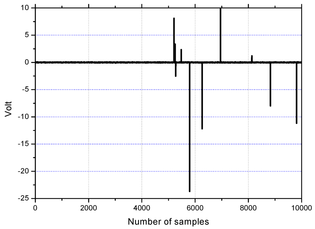
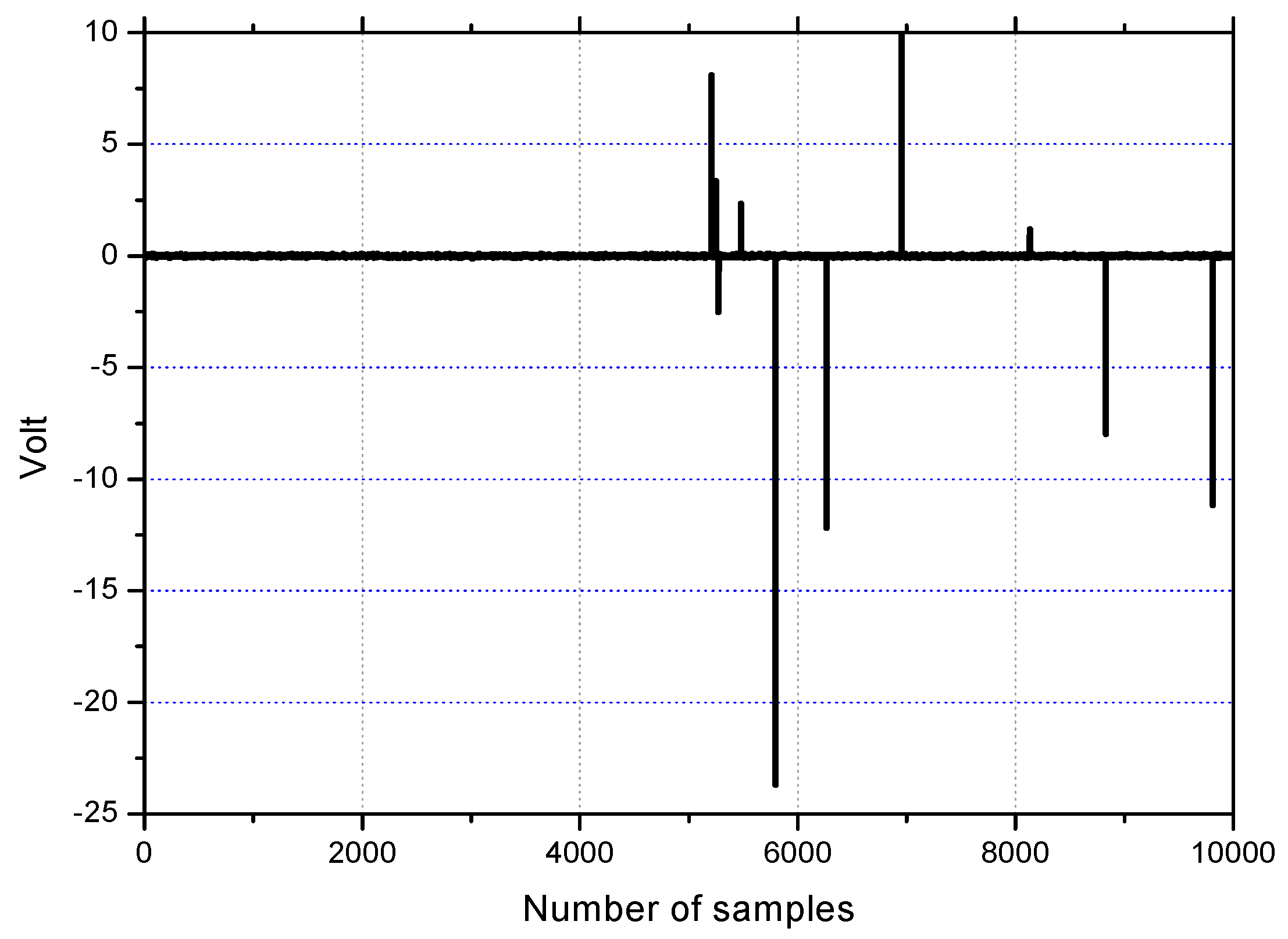
Firstly, the weight traces will be investigated through simulation in order to verify the property of robustness against impulsive noise. The impulses are generated with ε = 0.01 for clear observation of the weight behavior. The impulse noise as depicted in Figure 4 is applied to the channel output in the steady state, that is, after convergence.

Figure 4. The impulse and background noise for the simulation for the behavior of optimum weight.

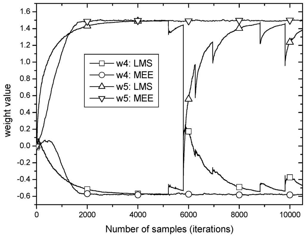
Figure 5 shows the learning curves of weight $w_{4,k}$ and $w_{5,k}$ (only two weights are chosen due to the page limitation). At around 5000 samples, both reach their optima completely, and then they undergo the impulsive noise like that in Figure 4. In Figure 5, it is observed that MEE and LMS have the same steady state weight values and each weight trace of MEE in the steady state shows no fluctuations remaining undisturbed under the strong impulses. This is obviously in contrast to the case of the LMS algorithm where traces of $w_{4,k}$ and $w_{5,k}$ have sharp perturbations at impulse occurrences and remain perturbed for a long time though gradually dying.

Figure 5. The behavior of weight values of w_4,k and w_5,k with impulsive noise being added in the steady state.

We can notice that the optimum weight of MEE has averaging operations and MCIE in (23) has some differences when the weight update Equation (8) is compared. Since the average operations can easily be defeated even by just one strong impulse, we can figure out that the dominant role of robustness against impulsive noise is the MCIE.

Secondly, the effectiveness of the proposed NMEE algorithm (25) designed with the MCIE is investigated through the learning performance comparison with the original MEE algorithm in (19) under the same impulsive noise with ${\sigma }_{IN}^2$ = 50 and ε = 0.03 as in the work [5] in which the impulsive noise is used in all time. The MSE learning results are shown in Figure 6.

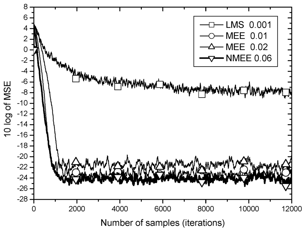
Figure 6. The Comparison of MSE learning curves under impulsive noise (square: LMS with μ_LMS = 0.001, circle: MEE with μ_MEE = 0.01, triangle: MEE with μ_MEE = 0.02, thick line: NMEE with β = 0.9 and μ = 6μ_MEE).

The LMS algorithm converges very slow and stays at about −8 dB of MSE in the steady state. This result can be explained from the expression of $W_{LMS}^{opt}$ in (8) having no measures to protect it from fluctuations from impulsive noise as discussed in Section 3. On the other hand, the MEE algorithm rigged with the magnitude controller for IE converges in about 1000 samples even under the strong impulsive noise. This result supports the analysis that the MCIE $X_{j,k}^{MCIE}$ keeps the algorithm (19) and its steady state weight undisturbed by large error values that may be induced from excessive noise such as impulses.

As for the performance comparison between MEE and NMEE in Figure 6, NMEE shows lower minimum MSE and faster convergence speed simultaneously. The difference of convergence speed is about 500 samples and that of minimum MSE is around 1 dB. When compared to the condition of the same convergence speed, the difference in minimum MSE is shown to be about 3 dB. This amount of performance gap indicates that the proposed method of tracking the power of MCIE recursively and using it in normalization of the step size is significantly effective in the aspect of performance as well as computational complexity.

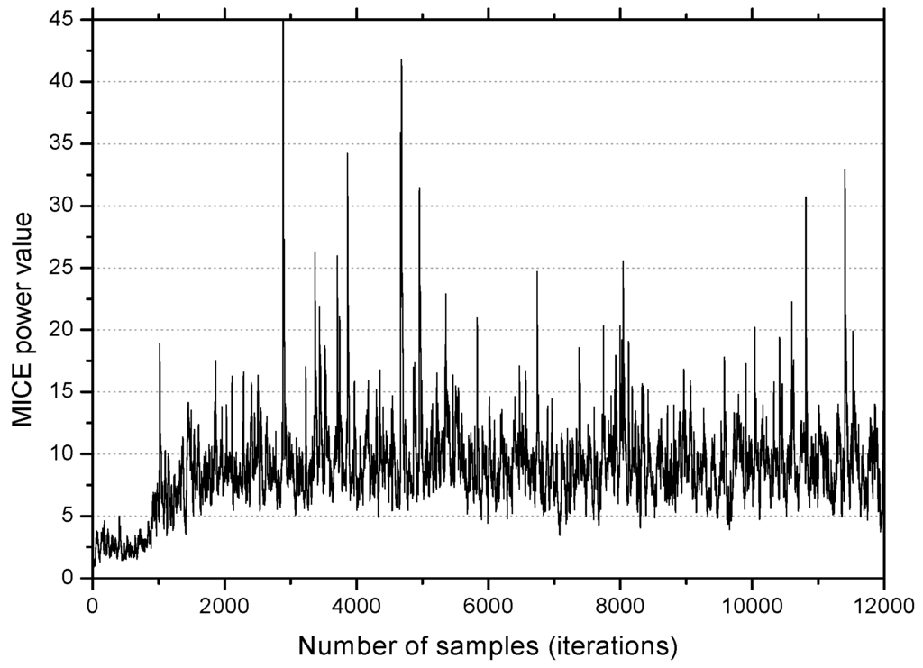
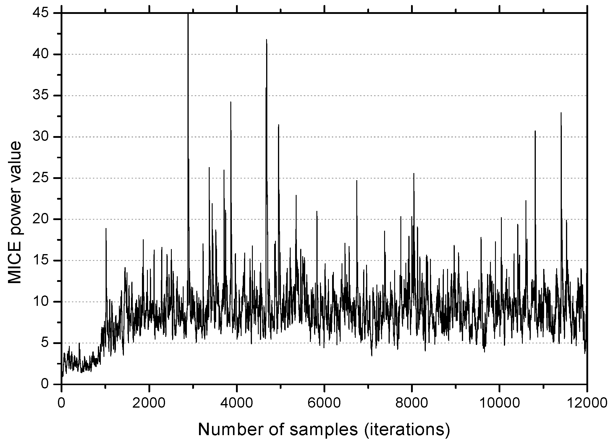
In Figure 7, the MCIE power becomes large as the MEE algorithm converges, and after convergence, the trace shows large variations, mostly above 6. The condition $P(k)>6$ in this simulation implies that when NMEE is employed, the value μ according to (32) must be greater than $6{\mu }_{MEE}$ for better performance. The fact that this is exactly in accordance with the choice $\mu =6{\mu }_{MEE}$ described in Figure 6 justifies the effectiveness of the proposed method by simulation.

Figure 7. The trace of MCIE power P(k) of the MEE algorithm under the same simulation conditions used for Figure 6.

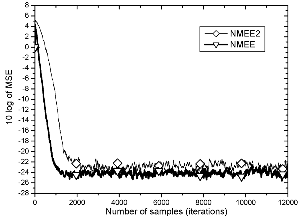
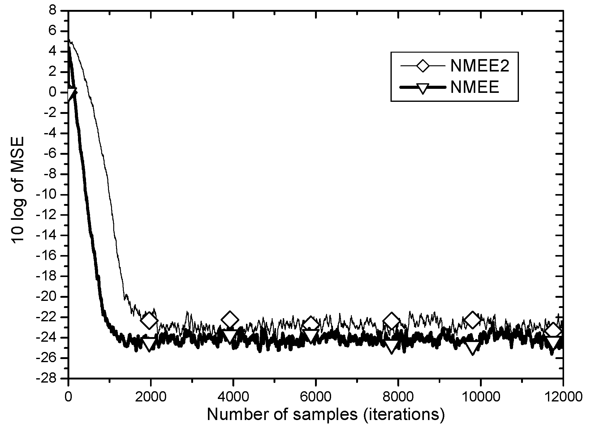
In the same simulation environment, the MSE learning curves for two input power normalization approaches, NMEE and NMEE2 are compared in Figure 8.

Figure 8. Learning curves of NMEE and NMEE2 algorithms for comparison of the two methods of input power normalization.

As observed in Figure 8, the input power normalization approach for variable step size selection for the MEE algorithm shows different MSE performances according to which signal power is normalized. When NMEE is employed where the magnitude controls input entropy, MCIE is used for power normalization, the MSE learning performance yields better steady state MSE of above 2 dB and faster convergence speed by about 1000 samples than when NMEE2 is adopted, in which the squared norm of the unprocessed input ${\Vert X_k\Vert }^2$ is used for normalization. As discussed in Section 4, under strong impulsive noise, the power of MCIE can be the right choice for step size normalization for better performance.

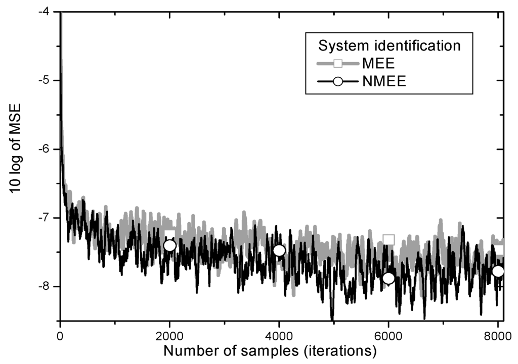
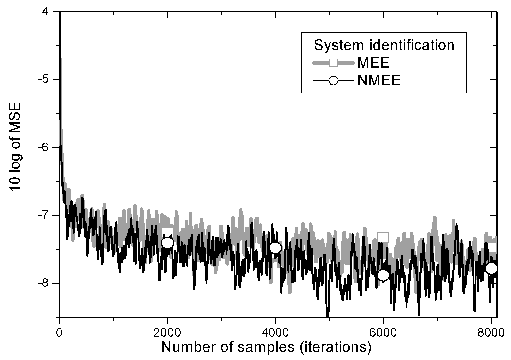
In system identification applications of adaptive filtering as appeared in the work [8], the desired signal is derived by passing the white Gaussian input through the unknown system. The unknown system in this simulation is of length 9. The impulse response of the unknown system is chosen to follow a triangular wave form that is symmetric with respect to the central tap point [9,13]. The TDL filter has 9 tap weights. The input signal is a white Gaussian process with zero mean and unit variance. The same impulsive noise used in Figure 6, uncorrelated with the input, is added to the output of the unknown system. MSE learning curves are depicted in Figure 9.

Figure 9. Learning curves of MEE and NMEE for system identification.

One can observe from Figure 8 that the proposed NMEE achieves lower steady-state MSE than the conventional MEE algorithm in the system identification problems as well.

6. Conclusions

The MEE algorithm is known to outperform MSE-based algorithms in most signal processing applications in an impulsive noise environment. The conventional MEE algorithm has a fixed step size so that it may require in practice to employ a time varying step size that appropriately controls its learning performance.

Based on the analysis of the behavior of optimum weight and the role of MCIE in mitigation of influence from large error, it was found in this paper that the NMEE employing the step size normalized with the power of the current MCIE element can yield lower minimum MSE and faster convergence speed simultaneously. On the condition of the same convergence speed, the performance enhancement of 3 dB in the equalization simulation leads us to conclude that the proposed method of recursive estimation of the MCIE power for normalization of the step size is significantly effective in both aspects of performance and computational complexity.

References

- Kim, N.; Byun, H.; You, Y.; Kwon, K. Blind signal processing for impulsive noise channels. J. Commu. Netw. 2012, 14, 27–33. [Google Scholar] [CrossRef]
- Armstrong, J.; Shentu, J.; Chai, C.; Suraweera, H. Analysis of impulse noise mitigation techniques for digital television systems. In Proceedings of the 8th International OFDM-Workshop, 2003, Hamburg, Germany, 24–25 September 2003; pp. 172–176.
- Santamaria, I.; Pokharel, P.; Principe, J. Generalized correlation function: Definition, properties, and application to blind equalization. IEEE Trans. Signal Process. 2006, 54, 2187–2197. [Google Scholar] [CrossRef]
- Erdogmus, D.; Principe, J. An entropy minimization algorithm for supervised training of nonlinear systems. IEEE Trans. Signal Process. 2002, 50, 1780–1786. [Google Scholar] [CrossRef]
- Kim, N. Decision feedback equalizer algorithms based on error entropy criterion. J. Internet Comput. Serv. 2011, 12, 27–33. [Google Scholar]
- Kim, N. Performance analysis of entropy-based decision feedback algorithms in wireless shallow-water communications. In Proceedings of KSII summer conference, Pyeongchang, Korea, 27–29 June 2012; pp. 185–186.
- Kim, N.; Andonova, A. Computationally efficient methods for decision feedback algorithms based on minimum error entropy. Available online: http://ecad.tu-sofia.bg/et/2014/ET2014/AJE_2014/017-A_Andonova.pdf (accessed on 23 June 2016).
- Wu, Z.; Peng, S.; Chen, B.; Zhao, H.; Principe, J. Proportionate minimum error entropy algorithm for sparse system identification. Entropy 2015, 17, 5995–6006. [Google Scholar] [CrossRef]
- Haykin, S. Adaptive Filter Theory, 4th ed.; Prentice Hall: Upper Saddle River, NJ, USA, 2001. [Google Scholar]
- Parzen, E. On the estimation of a probability density function and the mode. Ann. Math. Stat. 1962, 33, 1065–1076. [Google Scholar] [CrossRef]
- Chinaboina, R.; Ramkiran, D.; Khan, H.; Usha, M.; Madhav, B.; Srinivas, K.; Ganesh, G. Adaptive algorithms for acoustic echo cancellation in speech processing. Int. J. Res. Rev. Appl. Sci. 2011, 7, 38–42. [Google Scholar]
- Proakis, J. Digital Communications, 2nd ed.; McGraw-Hill: New York, NY, USA, 1989. [Google Scholar]
- Kim, N. A least squares approach to escalator algorithms for adaptive filtering. J. Commu. Netw. 2006, 28, 155–161. [Google Scholar] [CrossRef]
© 2016 by the authors; licensee MDPI, Basel, Switzerland. This article is an open access article distributed under the terms and conditions of the Creative Commons Attribution (CC-BY) license (http://creativecommons.org/licenses/by/4.0/).