Article

Stimuli-Magnitude-Adaptive Sample Selection for Data-Driven Haptic Modeling

Department of Computer Engineering, Kyung Hee University, Yongin-si 446-701, Korea
*
Author to whom correspondence should be addressed.
Entropy 2016, 18(6), 222; https://doi.org/10.3390/e18060222
Submission received: 19 April 2016 / Revised: 1 June 2016 / Accepted: 2 June 2016 / Published: 7 June 2016

Abstract

:
Data-driven haptic modeling is an emerging technique where contact dynamics are simulated and interpolated based on a generic input-output matching model identified by data sensed from interaction with target physical objects. In data-driven modeling, selecting representative samples from a large set of data in a way that they can efficiently and accurately describe the whole dataset has been a long standing problem. This paper presents a new algorithm for the sample selection where the variances of output are observed for selecting representative input-output samples in order to ensure the quality of output prediction. The main idea is that representative pairs of input-output are chosen so that the ratio of the standard deviation to the mean of the corresponding output group does not exceed an application-dependent threshold. This output- and standard deviation-based sample selection is very effective in applications where the variance or relative error of the output should be kept within a certain threshold. This threshold is used for partitioning the input space using Binary Space Partitioning-tree (BSP-tree) and k-means algorithms. We apply the new approach to data-driven haptic modeling scenario where the relative error of the output prediction result should be less than a perceptual threshold. For evaluation, the proposed algorithm is compared to two state-of-the-art sample selection algorithms for regression tasks. Four kinds of haptic related behavior–force datasets are tested. The results showed that the proposed algorithm outperformed the others in terms of output-approximation quality and computational complexity.

Graphical Abstract

1. Introduction

In the last couple of decades, owing to its remarkable developments, virtual reality (VR) systems have found applications in most scientific fields. A key aspect of VR is the provision of a high level of realism where the user can act and behave in a life-like manner. Recently, VR has received tangibility due to the inclusion of haptic feedback, which improved the realism and immersiveness of the system.
In general, the haptic feedback is calculated via physics simulation that determines the feedback based on haptic models for the simulation and user’s actions. The haptic model can be either physics based [1,2,3,4,5,6,7] or generic interpolation models [8,9,10]. The models for simulation can also be either manually built or identified based on real measurement [11,12]. In particular, measurement-based modeling using a generic interpolation model, namely data-driven modeling, is emerging in the haptics research field [8,9,10]. This can prove highly beneficial for people with special needs [13]. In this approach, input-output data pairs collected with sensors, are pre-processed, e.g., sample selection, and are fed into the interpolation model training algorithm. The trained interpolation model is used for predicting output based on interactive inputs during rendering. Data-driven approaches can deal with very complex behaviors, e.g., inhomogeneous stiffness with large deformation, using a relatively simple and unified framework.
One of the challenging parts is to ensure the quality of input-output data for interpolation model training. The data should be sufficient in terms of quantity and the area of coverage in the input space. That is, the data pairs should thoroughly cover the all possible interactions to ensure the quality of the model and presumably the quality of the output prediction. A simple solution for this is to increase the number of data samples. However, without careful sample collection, some of these data points can be redundant and do not provide any additional information. Moreover, increased amounts of data inherently escalates the time taken for training and rendering. More seriously, when the dimension of input space increases, the data points needed to sufficiently cover the input space increase exponentially, which makes the training infeasible.
In order to overcome this, it has been proposed that only a part of the whole data set be appropriately selected and used for training [14]. In data-driven haptic modeling, a few groups are leading this research. For example, Hover et al. [14,15] designed a sample selection algorithm based on k-d (k-dimensional) tree data structure for non-linear force feedback approximation, which provided good results for rendering [14]. However, it tends to over segment in the low reference force range. They used perceptual criterion, i.e., force perception Just-Noticeable-Difference (JND) curve, in the selection process, and the forces below 0.1 N were not considered. Additionally, the algorithm relies on the results from the approximation algorithm in each iteration. This shows that the algorithm is dependent on the approximation algorithm, and it cannot be generalized for use with most other approximation algorithms. Additionally, since the whole signal had to be reconstructed in each iteration, the time complexity was also increased. More recently, Arnize et al. proposed Discretization-based Condensed Nearest Neighbor (D-CNN) and Discretization-based Edited Nearest Neighbor (D-ENN) as modified versions of Condensed Nearest Neighbor (CNN) and Edited Nearest Neighbor (ENN) for regression tasks [16]. Both of the algorithms ensure a balanced selection of samples throughout the sample space using equal-width binning of the uni-dimensional output signal. This strategy ensures a low absolute error on the output estimates, but the relative error can be inflated in the low reference stimuli range.
In the present work, we propose a novel sample selection algorithm, namely SMASS (Stimuli-Magnitude-Adaptive Sample Selection), where the ratio between the standard deviation and the mean for the output group is kept nearly constant. This approach is especially useful for haptic modeling where the relative errors on the output predictions are needed to be kept below the human perceptual discriminability that changes proportionally with the reference stimulus magnitude. The algorithm is implemented with BSP-tree partitioning [17] of the input space using k-means guided by corresponding output groups, which significantly increase efficiency of the modeling in terms of the time taken to build the models. The main characteristics of the proposed algorithm are as follows:
-
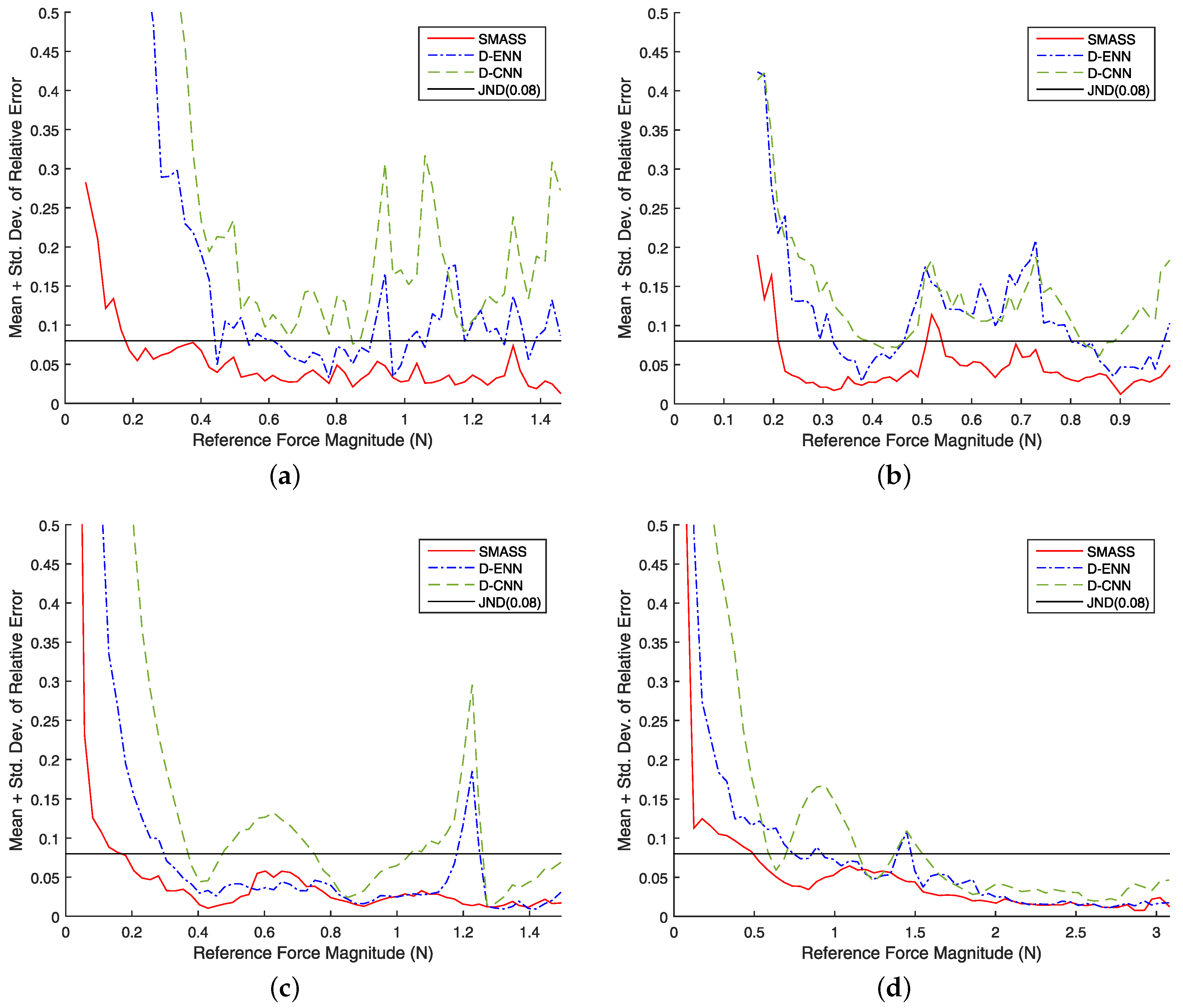
SMASS selects a high number of representative points when the reference stimulus is low, while it selects a low number of points when the reference stimulus is high, which fits well to the human perception characteristic: stimuli difference in small magnitude is more prone to be detected than that in large magnitudes, e.g., humans can detect the difference between 0.3 N and 0.5 N but cannot do it between 30.3 N and 30.5 N (see Section 5 for more details).
-
SMASS processes multivariate output as a whole, unlike most other algorithms that work with uni-dimensional projections of multivariate output data (one at a time). This significantly increases the training efficiency when there are multiple dimensions in output.
-
The computation speed of the proposed algorithm is very high due to its simplicity and the use of the binary partitioning approach.
-
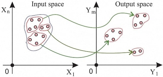
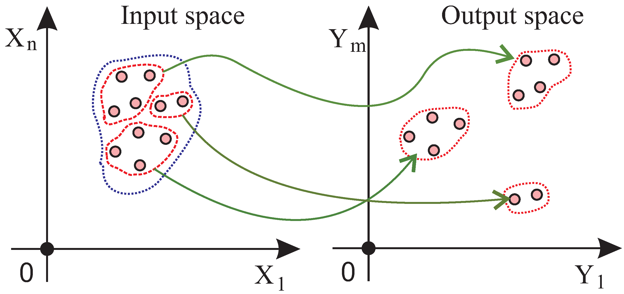
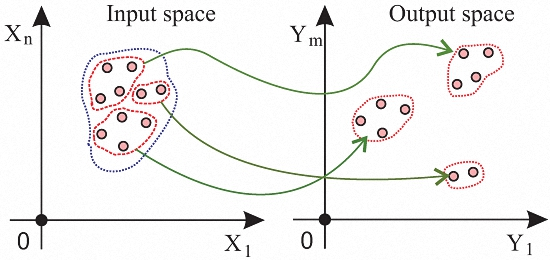
Unlike previous approaches, both the input and output and their relationship are used for the selection of representative samples. This allows an appropriate sample selection in the case when closely clustered input points are mapped to sparsely distributed output points, and vice versa. Previous approaches that only see input or output would fail to capture the relationship in such cases.
The rest of the paper is structured as follows. The literature review is provided in Section 2. The algorithm is described in Section 3. Then, the datasets and the data recording setup are described in Section 4. The discussion in Section 6 is provided based on experimental results and evaluation from Section 5. Finally, the paper is concluded in Section 7.

2. Related Works

Sample selection techniques are used to reduce the size of the dataset while preserving the characteristics of the entire dataset. This reduction in size leads to increased efficiency, reduced storage, and decreased computational complexity. A variety of approaches have been proposed for this purpose with applications across different research areas. For example, in the field of computer vision, researchers used sample selection algorithms for scene categorization in images and videos [18,19,20]. Evolutionary algorithms for sample selection were used for text classification and traffic sign recognition in [21,22], respectively. Sample selection algorithms are readily used in medical datasets in [23,24]. However, sample selection techniques find most usage in the field of data mining. The authors in [25,26] used scalable sample selection algorithms for dealing with very large scale datasets. Furthermore,[27] also provides a data condensation algorithm for large datasets in machine learning.
For an overall view, the authors in [28,29,30] provide a taxonomy for the methods used for sample selection, where the methods are classified on the basis of differences in type of selected samples, direction of search for selecting samples, and evaluation of search. Previously, most of the sample selection algorithms were used for classification of the dataset into sub-classes. This approach works well only when the dataset is discrete and fails when the algorithms have to predict a continuous output. Additionally, the number of sub-classes to be predicted are also very low. In order to tackle a continuous output and achieve a higher number of sub-classes, recent research has focused on using regression for prediction.
The first usage of regression for sample selection can be accredited to [31]. Afterwards, the authors in [32] used genetic algorithms for detection of outliers and sample selection in linear regression models in the context of cross-section data. In [33], sample selection was carried out in the framework of Multi Objective Evolutionary Learning (MOEL) of Fuzzy Rule-Based Systems (FRBSs) by using a co-evolutionary method. With a reduced sample set of 10% and 20% of the overall dataset, they were able to get results that were almost comparable to the results from the whole dataset. The computation time was also reduced by over 85% with the reduced dataset. Recently, researchers have used sample selection techniques, which were mainly applied to classification problems, for regression tasks. In [34,35], the authors proposed algorithms which used modified versions of Edited Nearest Neighbor (ENN [36]), Condensed Nearest Neighbor (CNN [37]), and CA [38] for sample selection for regression. Another sample selection method, Class Conditional Instance Selection (CCIS [39]), was modified for regression tasks in [40] and was applied for reducing variance in Genetic Fuzzy Systems (GFSs). Furthermore, in [41], a simpler and more robust sample selection algorithm is proposed for noise filtering. The main advantage of this method is that it can be applied to any sample selection approach. Afterwards, the output is discretized into a predefined number of quantization levels for regression purposes.
Recently, the authors in [16] used modified versions of CNN and ENN for regression. Two strategies were presented; threshold-based (T-CNN, T-ENN), and discretization-based (D-CNN, D-ENN). The threshold-based method is density driven. It selects or rejects samples based on the comparison of error between given and predicted output values with a threshold value, while, in the discretization-based method, the output is discretized into evenly spaced levels by employing equal-width binning using leave-one-out estimated entropy technique.
Sample selection algorithms are used in various research fields; however, one common aspect of all these algorithms is that they consider uni-dimensional projections of the output, which considerably decreases the computational efficiency of the system in the case of multi-dimensional output. The proposed algorithm tackles this problem by processing the output as a multivariate signal.
Another important aspect for sample selection algorithms is the structure or distribution of data points in space. Most of the algorithms assume that the data is homogeneously distributed or clustered into separable groups. However, this might not be the case in most real-world scenarios. In order to consider the effect of inhomogeniety of the data points, Li et al. in [42] considered the Local Probabilistic Centers (LPC). The LPC was modified for higher dimensional datasets in [43]. In [44], Wen et al. presented a new algorithm called Relative Local Mean Classifier (RLMC) for dealing with sparse high dimensional data. They transformed the Local Mean Classifier (LMC) [45], using Euclidean distance, in accordance with the human visual perception ability for better classification. This algorithm was further improved by considering the densities of classes in [46]. Furthermore, the authors in [47] presented a new algorithm where dense regions were identified and an effort was made to select fewer samples from those regions to avoid overfitting. In [48], the presented algorithm gathers useful information from the neighborhood and heuristically organizes the local distribution characteristics for faster classification accuracy and speeds.
Furthermore, most of the previous sample selection algorithms are used for classification purposes, which are difficult to be directly applied to data-driven haptics where sample selection is used for regression purposes. The present algorithm can be directly applied to this regression task. There are a few algorithms for regression tasks. Among them, the state-of-the-art work was introduced in [16]. However, this algorithm again focuses on maintaining an absolute error, instead of a relative error. A new approach is needed for the case where perception-related relative error is important.

Sample Selection in Haptics

In data-driven haptic modeling for virtual reality, which is closely related to the present work, little research exists. For example, in order to deal with object inhomogeneity, Sianov et al. segmented the dataset into relatively homogeneous regions during initial scanning phase [49]. Then, each region was represented with a single set of data-points. The training complexity of their interpolation model, i.e., radial basis function model, was reduced by applying l 1 minimization technique.
In [15], the authors proposed three techniques for input-output point selection for non-linear force feedback rendering incorporating visco-elastic nature of a soft body. The technique that provided the best approximation was the k-d tree selection algorithm [14] which was adopted from the quad-tree method in [50]. The barycenters of each leaf of the k-d tree form the representative set of samples. The algorithm starts with an initial partition into two leafs and stops when the number of leaves reach the desirable number of samples. The leaf that contains the worst approximated sample relative to the force JND curve becomes a candidate for bisection.
Some parts of the above mentioned algorithms are dependent on approximation algorithm, and thus it is sometimes not easy to apply the algorithms to general data-driven modeling. Thus, one of the goals of the present work is to make a more general sample selection algorithm for data-driven modeling. Additionally, in [14], the authors did not consider the forces below 0.1 N due to an over segmentation problem in the low reference force range. The present algorithm solves this by a magnitude adaptive sample selection strategy.

3. Stimuli-Magnitude-Adaptive Sample Selection Algorithm

3.1. Problem Definition and Approach

The core part of data-driven modeling is to train an interpolation model for mapping the input dataset to the output dataset. The input points are sometimes gathered in a distinct group inside the input space, whereas the corresponding output samples are scattered, or the other way around, as shown in Figure 1. In this case, the sample selection strategy that observes only an input or only an output set of data-points might provide a poor or even wrong set of representative samples. Instead, the input grouping can be guided by corresponding output distributions, as an additional source of information for selection procedure. In this section, we propose a novel sample selection algorithm that selects a representative set of input-output pairs based on ties between input and corresponding output groups of points.
Suppose that all the input samples, S R n , can be divided into i groups, S i , which can be represented by a single vector, e.g., mean sample of S i . Then, in order to select representative input-output pairs, the corresponding groups T i from the output set T has to form distinct groups. In addition, each group must show a relatively low variance. A relatively high variance of T i indicates that the data points are dispersed in the output space, which reduces applicability of the single input-output pair as representative. The first constraint for this algorithm is to partition the set S, so that the ratio of the standard deviation to the mean of corresponding subsets T i is less then or equal to a threshold τ, such that,
P = { T i | σ i μ i τ , i = 1 , , k } ,
where P is a set of k clusters that corresponds to the grouping of the input space S k . The standard deviation and the mean of subset T i are denoted as σ i and μ i , respectively. The number of representative pairs k varies in the range from 1 to the number of elements.
The second constraint for this algorithm is to find the minimal number of clusters k from the set S so the corresponding clusters from T meet constraints in Equation (1). This minimum number is the bottom line which merely guarantees a τ degree of accuracy. Once the minimal set of clusters satisfying Equation (1) is selected, representative data pairs can be selected based on a predefined rule, i.e., points closest to the mean from S i and T i .
The first constraint uses the standard deviation to the mean ratio to ensure that the relative error remains under the threshold τ. For example, a group of samples having a standard deviation of two has a more pronounced effect if the mean value is 10 as compared to a mean value of 100. Therefore, it is important to use this ratio in applications where the relative error has to be kept under a specific threshold. Specifically, in the field of haptic perception, the difference between two stimuli, to be perceptually discriminable, increases with the magnitude of the stimuli.
The second constraint is used for minimizing the total number of clusters. The constraint tries to reduce the number of clusters while upholding the first constraint. Thus, the best solution is the one where ratio of standard deviation to mean tends to τ for all clusters.
In order to partition the input space while fulfilling the constraints, we need appropriate data structure to (1) efficiently manage the search for the minimal number of groups; and (2) determine appropriate partitioning strategy. The next section explains how our algorithm deals with these requirements in a unified framework.

3.2. Algorithm

The input space can be partitioned and stored in different ways. The most common technique used for this purpose is the use of the tree data structure. In this research, we used the BSP-tree technique. It organizes the input into a form where each node is linked to a set of patterns (clusters). Binary partitioning is carried out at each node until each leaf node is associated with a single data pattern. The nodes store parameters related to the associated patterns which help in increasing the computation speed of each iteration.
BSP-tree [17] and other such algorithms are used as a pre-processing step for k-means. According to [51] the partitioning policy of BSP-tree (approximate hierarchical clustering) provides a higher quality tree with higher intra-partition similarity that allows k-means to converge quickly. The BSP-KM (Binary Space Partitioning K-Means) algorithm shows better scalability, lower computation time, and higher efficiency, as compared to the k-d tree algorithm, as the dimensionality of the data space increases. Motivated by the BSP-KM algorithm, we decided to use the BSP-tree to store the input partitions, and k-means algorithm for leaf partitioning.
In this work, we redesigned the BSP-KM to find the optimal number of representative pairs from S and T, that are conditioned by Equation (1). The algorithm starts with partitioning the input space into two sets using the k-means clustering technique. In accordance to the sample indexes in each group of S k , the algorithm classifies the elements of the set T k . Afterwards, the mean and standard deviation are calculated for each T i . If the ratio of the standard deviation to the mean of the group is less or equal to the threshold value τ, the element closest to the mean of each cluster in T i and the corresponding element from S i of the leaf are marked as a representative pair. Otherwise, the algorithm continues to split the leaf recursively. The algorithm stops partitioning when all leaves from T k meet the above mentioned condition. The final step is the traversal of the tree and extracting the marked pairs. Thus, in the form of representative pairs, we select a subset of the overall dataset. Algorithm 1 shows the pseudo code for the proposed algorithm.
Using the ratio of the standard deviation to the mean of the group, as a termination criteria for selection algorithm, has one critical drawback. When the mean is equal to or very close to zero, the algorithm tends to over segment. The number of selected samples might increase in a way that all the samples close to zero are selected. In order to prevent this over sampling, an additional threshold ψ is introduced. The threshold ψ defines the level below which the mean value of T i is considered as zero. Once the mean value of a given cluster is defined to be below ψ, the decision about partitioning depends on the value of μ i + σ i . If the value of μ i + σ i is higher than ψ, partitioning continues. Otherwise, the algorithm stops and returns the mean points of S i and T i as representatives.
The value of ψ is dependent on the type of application and data. For example, in certain cases, a value of 0.1 can be considered as a zero value, while in other cases, a value of 0.01 can also be considered as a significant value. In the case of haptic applications, it is recommended to select ψ according to the absolute threshold of haptic perception. Absolute threshold is the minimum amount of stimulus that can be perceived by a human.
Entropy 18 00222 i001

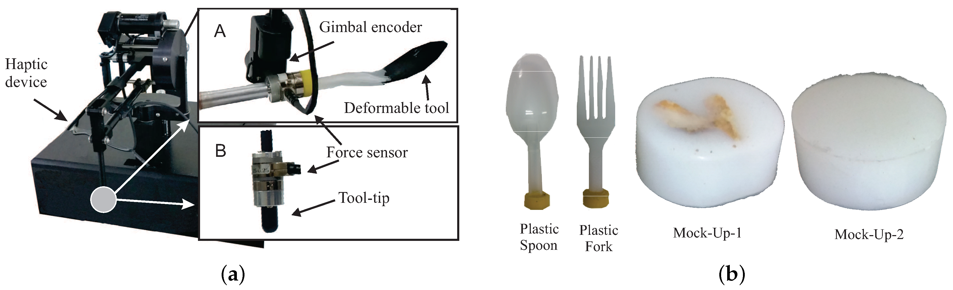
4. Dataset Collection and Recording Setup

The proposed algorithm is evaluated in a typical haptic interaction scenario where a user (holding a rigid tool) is touching a deformable object or a user is holding a deformable tool touching a rigid object. The data input used in the scenario is multiple three-dimensional vectors capturing user’s movement, and the output is the corresponding reaction force vector due to the stiffness of the touched object. We selected this scenario since the haptic rendering of a deformable object is one of the most challenging tasks in the haptics field, and the data-driven approach has proved to be the most proper solution [10]. Since we are dealing with multiple three-dimensional vectors, a large amount of data captured should be processed in the training. This scenario can be considered as a good example for testing the algorithm.
The algorithm was evaluated with four different haptic datasets. Two datasets were collected from deformable tools, i.e., a plastic spoon and a plastic fork, by palpating a rigid surface with the tools (see Figure 2b). The other two were collected from deformable objects i.e., mock-up-1 and mock-up-2 (see Figure 2b). Data were recorded by palpating each deformable object with an 8 mm rigid tool.
In order to collect data for our experiment, a data acquisition setup was built, as shown in Figure 2a. We collected two three-dimensional vectors for capturing user’s movement: initial contact position and displacement vector. The former is the position of the tool tip at the moment of initial contact and plays the role of a reference point for the deformation. The latter is the relative distance between the initial contact point and the current tool tip, which represents the degree of deformation. Both the position data are measured using the position sensing capability of the haptic interface (PHANToM Premium 1.0; Geomagic Inc., Rock Hill, SC, USA). The position sensing resolution is 0.03 mm. Different tools for interaction (see Figure 2a) were attached to the PHANToM end effector for data recording. The three-dimensional force signal at the tool tip was captured using a force/torque sensor (Nano17; ATI Technologies, Markham, ON, Canada) attached to the tools. The signal from both sources was recorded at 1 kHz using NI DAQ acquisition board (PCI-6220; National Instruments, Austin, TX, USA).
The data recorded from these datasets were in the form of input-output pairs. The output from all the datasets was a three-dimensional force vector, whereas the input data varied depending on the scenario. The displacement vector for the deformable tool scenarios (spoon and fork) was calculated by measuring the distance of the tool tip between the initial contact point and the imaginary tool tip position if there was no deformation. For the deformable object scenarios (with rigid tools) the displacement vector was calculated by measuring the distance between the tool tip and the initial contact point. Thus, each dataset consisted of six input attributes and three output attributes.
The dataset from the spoon scenario represents general non-linear input-output mapping. A total of 3843 data points were collected. The dataset from the fork scenario shows a more complex behavior than the spoon due to the self-collision of its tines. A total of 3419 data points were collected. Mock-up-1 was made from silicon with stones embedded inside it, which alters the homogeneity of the mockup, making the input-output relationship more complex. The size of the dataset was 8375. Mock-up-2 was made purely from silicon, and the main characteristic of this dataset was to cover a larger scanning area with varying speeds and palpation durations. This strategy made the dataset relative larger than the others (21,537 data points), which will be available at an external link [52].

5. Experimental Evaluation

Since the proposed algorithm falls into the category of sample selection for regression tasks, two recent algorithms D-ENN, and D-CNN [16] were selected for comparison. Along with the above mentioned algorithms, Arnaiz-González et al., also proposed threshold based algorithms i.e., T-ENN, T-CNN, and their ensembles. However, during our pilot tests, the latter algorithms showed a relatively low compression ratio (large number of selected points) as compared to other algorithms, including the proposed algorithm. The requirement of a low number of selected samples was imposed due to the fact that these samples are involved in real time approximation in rendering. Additionally, since the datasets were related to haptics where a minimum update rate of 1 kHz is required, the acquisition of a low number of selected samples was paramount. These reasons contributed towards the exclusion of the T-ENN, T-CNN, and their ensemble algorithms from the comparison for evaluation.

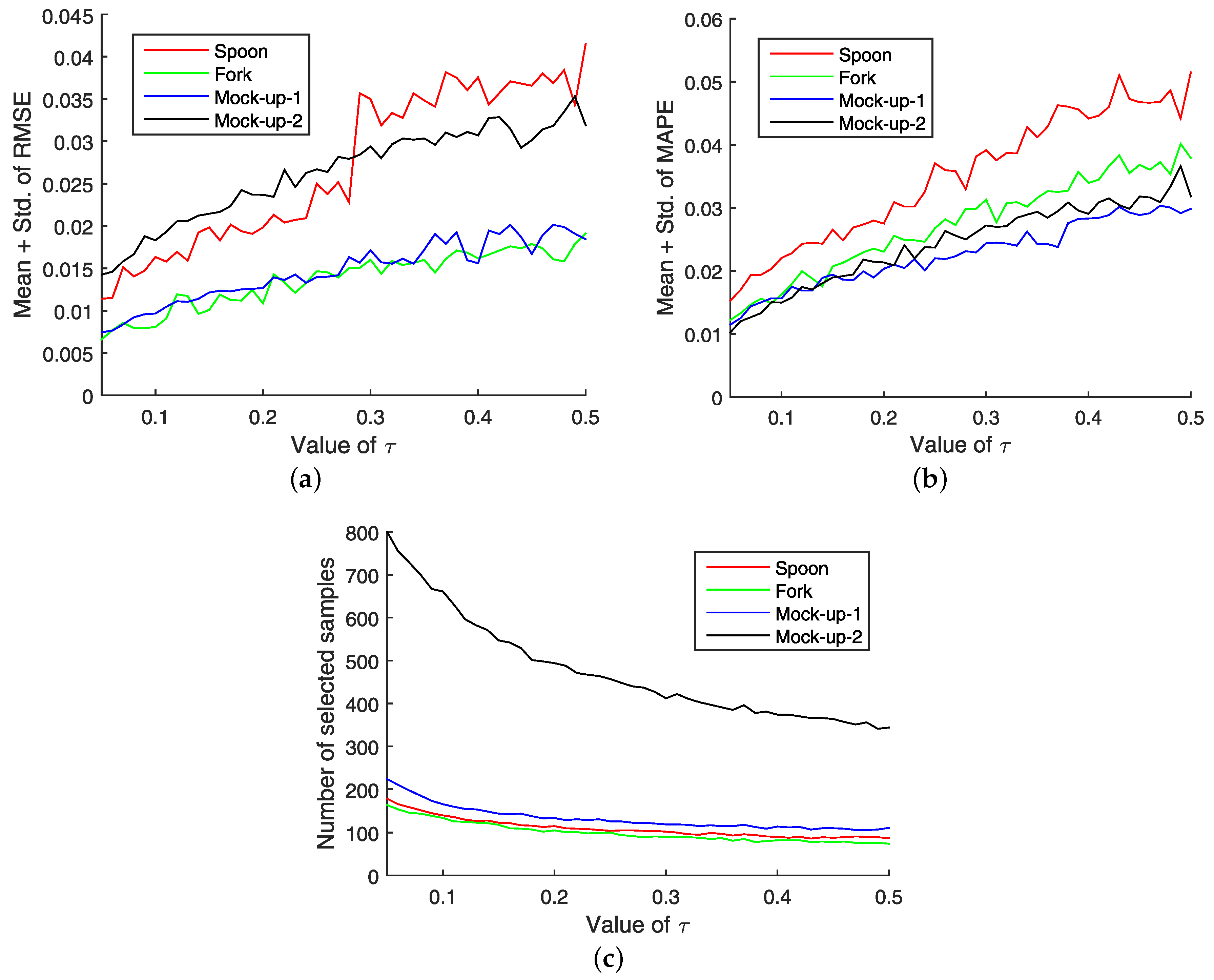
5.1. Parameter Selection
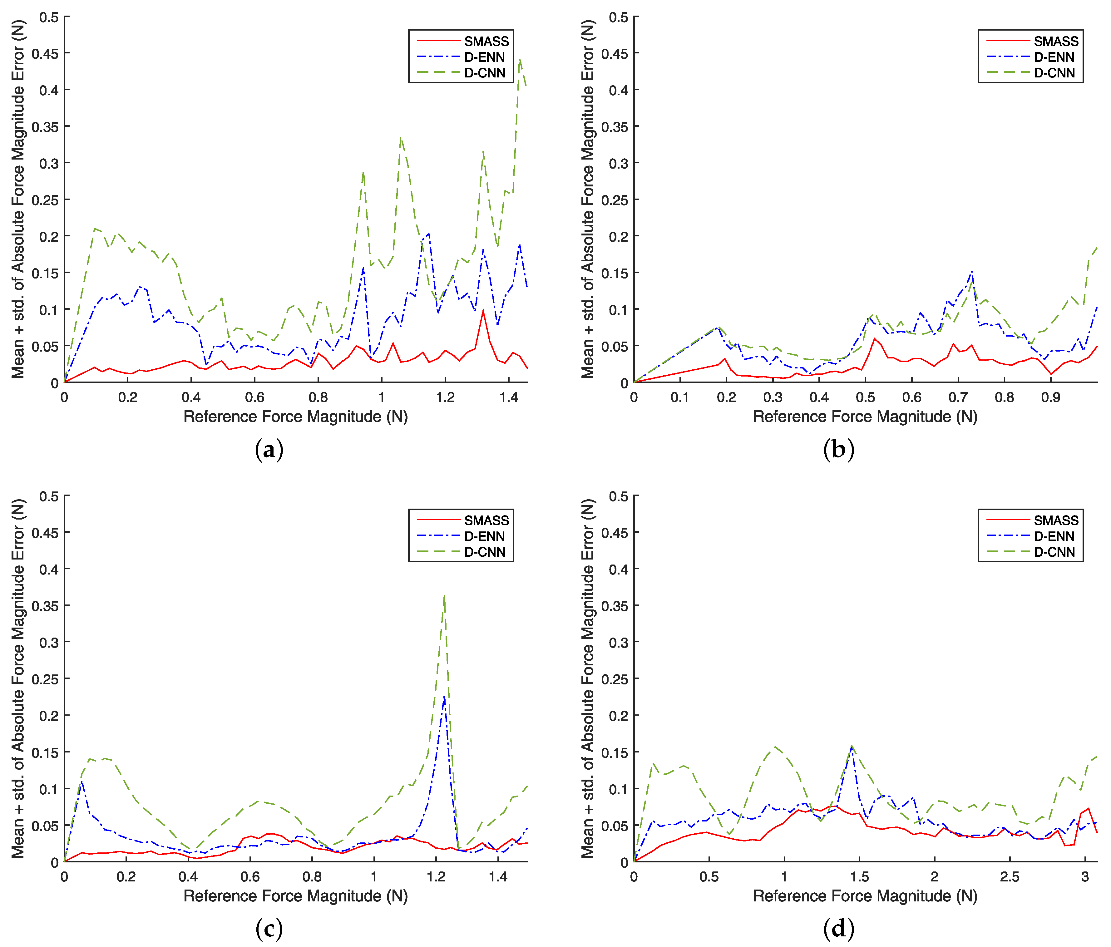
For evaluation purposes, the threshold value τ should be determined according to the application and the nature of data. In order to find the optimal value of τ for our application, we analyzed the effect of τ on relative force magnitude error in prediction (as shown in Figure 3a), absolute force magnitude error in prediction (as shown in Figure 3b), and the number of selected samples (as shown in Figure 3c). It was found that the value of τ is positively correlated with the absolute and relative errors of reconstructed signal and negatively correlated with the number of selected samples. Thus, the value of τ is a trade-off between the number of selected samples and the error rate. The value of τ can be tuned to achieve a certain number of representative pairs or to minimize the error rate of reconstructed signal to a certain level.
Figure 3c shows that the decrease in the total number of selected samples with the increasing value of τ is not significant after τ equals 0.2, whereas the error values constantly increase with the increase in the value of τ. Thus, selecting a value of τ greater than 0.2 proved less beneficial for the given datasets, as the reduction in the number of samples was less significant as compared to the increase in the error values. Therefore, it was decided to set the value of τ at 0.2. This value is considered as optimal for the current datasets, but the value of τ for other datasets can also be calculated in a similar fashion.
Since we are dealing with haptic force perception, the threshold value for ψ can be selected as 0.03 N following the absolute threshold of human perception [53]. The absolute threshold is the minimum amount of force that a human can perceive. After setting the thresholds, the proposed algorithm was used to determine the number of selected samples.
A special effort was made to choose an equal number of selected samples for all the algorithms to provide a level ground for comparison. The parameters of the other algorithms were tuned to make the number of selected samples approximately equal, while maintaining a high approximation quality. These parameters included the number of discretization levels and k for the underlying k-NN algorithm. This ensured that, besides the desirable number of samples, the best possible selection accuracy is achieved. Additionally, D-ENN and D-CNN can only work with a uni-dimensional output space; therefore, each dimension of the three-dimensional space was used iteratively, one at a time. The final number of selected samples is shown in Table 1.

5.2. Results

All of the algorithms, including the proposed algorithm, were implemented in MATLAB™ (R2014b), Natick, MA, USA, to provide a fair basis for comparison. The speed of D-ENN and D-CNN algorithms depends on the computational complexity of the underlying k-NN algorithm. Therefore, the k-d tree data structure was used for accelerating the k-NN algorithm. On the other hand, the speed of the proposed algorithm depends on the speed of BSP-tree leaf partitioning. For achieving a high computation speed, k-means + + algorithm [54] was used. The k-d tree and k-means + + are available in MATLAB™.
For all of the algorithms, the radial basis function network (RBFN) was chosen as a base model for output signal approximation. Selected data points by sample selection algorithms were considered as the centers for RBFN. The cubic spline technique was selected as the kernel for RBFN. A weight vector and a polynomial term for RBFN was obtained using a SpaRSA algorithm [55]. The time for RBFN training and approximation was not included for evaluation.
The performance results for all the algorithms were achieved using ten-fold cross validation. Each dataset was randomly partitioned into ten equal sized groups, where nine groups were used for training and one group was used for testing. The process was repeated ten times so that each group was used for testing. The Mean Absolute Percentage Error (MAPE), Root Mean Square Error (RMSE), and the average computation time are provided in Table 2. Both RMSE and MAPE were calculated based on the magnitude of three dimensional error vector, i.e., the vector pointing from reference data point to the approximated one in the three-dimensional space. The relative force magnitude error is depicted in Figure 4. The absolute force magnitude error can be seen in Figure 5. It is evident from Figure 4 that the relative error value for the proposed algorithm mostly lies below the value of 8%. This 8% is the approximate value of haptic force JND, which does not vary with test conditions, body sites or reference force [56,57]. JND is the minimum amount of difference between two stimuli due to which they are perceived as different from one another. This rule was first proposed in [58], where it was stated that JND depends on the intensity of the reference stimuli while the ratio (d) between the difference in stimuli to the reference force (d = ΔI/I) remains constant over a wide range of intensities. The fact that humans cannot distinguish between forces that fall inside the JND threshold, shows that it is possible to eliminate such forces from the data without compromising on the quality of perception. The algorithms for which the relative error in the reconstructed signal falls below the JND are considered as suited to haptic applications.

6. Discussion

The relative error of proposed algorithm showed the best results across every dataset. Just a single spike appeared above the JND level for the fork dataset only. For the spoon dataset, the proposed algorithm considerably outperformed the others, especially for low reference forces in terms of relative error magnitude. Similarly, the stability of the proposed algorithm was better through out the force range, more so in the higher reference force range for the spoon dataset. The D-ENN algorithm showed weaker performance for low reference force along every dataset in comparison to the proposed one. It is worth considering that, in case of the Mock-up-1 and Mock-up-2 datasets, the D-ENN and the proposed algorithm are comparable for high reference forces. However, several spikes appear on the relative error curve of D-ENN for high reference forces for most datasets, which causes instability. The D-CNN showed the worst results for relative errors across every dataset.
The absolute error in reconstructed signals for the proposed algorithm showed stable error rates along the whole range of forces. Only a few low magnitude spikes can be seen for forces higher than 0.4 N in the fork and spoon datasets. The proposed algorithm shows lower absolute error values, both for low and high reference forces, as compared to other algorithms across all the datasets. Similarly, the curve for the absolute error of the proposed algorithm shows higher stability. The worst result was exhibited by D-CNN algorithm, especially for low reference forces. The absolute error curve for D-ENN shows sudden spikes for all of the datasets. Summarizing the results of the absolute error, we can conclude that the proposed algorithm showed the best results for low and high reference forces. However, for the high reference forces, the D-ENN algorithm showed comparable results to the proposed algorithm only in the Mock-up-2 dataset.
Computational time is another aspect that was observed for all of the algorithms. The time for sample selection increases significantly for D-ENN and D-CNN with increasing number of samples in the set. In this regard, the proposed algorithm outperforms the other two algorithms significantly. The Mock-up-2 dataset contained the most samples, and the proposed algorithm completed the sample selection task within eight seconds, while it took around 46 minutes for D-ENN and around nine minutes for D-CNN to complete the said task. Details of the computation time for all the algorithms across all datasets are provided in Table 2. Thus, for bulky sensory data, the proposed algorithm easily outperforms the others.
The proposed algorithm is revealed as the most suitable for data-driven haptic modeling. It showed the best performance for all datasets with the lowest relative and absolute errors (see Table 2). The D-CNN and D-ENN algorithms showed relatively poorer performance on our datasets.

7. Conclusions

In this paper, a new algorithm was proposed for sample selection where representatives were selected based on the ratio of standard deviation to the mean of a particular group of samples. Such a strategy reduces the relative error by selecting more representatives from the low reference stimuli region and selecting a low number of representatives from the high reference stimuli region. The proposed algorithm was compared with two state-of-the-art algorithms for sample selection. The results showed that the proposed algorithm outperformed the other algorithms across all the datasets.
Furthermore, the computational complexity of the proposed algorithm was significantly lower. The significance of the proposed algorithm is that it can be used in any system where human perception is involved. The algorithm finds its most application in virtual and augmented reality systems.
Selecting an optimal value for the threshold proved to be a critical step in the algorithm. Currently, this value was selected analytically for the given datasets. As a future work, we would like to incorporate our algorithm with a dataset invariant threshold selection mechanism so that the algorithm can specify the thresholds without user intervention.
Furthermore, we would like to find the extent to which we can automate our algorithm, as in certain cases human intervention proves more beneficial [59].

Acknowledgments

This research was supported by the Global Frontier Program (NRF-2012M3A6A3056074) and the ERC program (2011-0030075) both through NRF Korea, and by the ITRC program (IITP-2016-H8501-16-1015) through IITP Korea.

Author Contributions

Arsen Abdulali and Seokhee Jeon conceived the idea and design. Arsen Abdulali and Waseem Hassan performed the experiment. Seokhee Jeon analyzed the data. Seokhee Jeon and Waseem Hassan prepared the datasets. Waseem Hassan and Arsen Abdulali wrote the paper. All of the authors read and approved the final manuscript.

Conflicts of Interest

The authors declare no conflict of interest.

References

  1. Lin, M.C.; Otaduy, M. Haptic Rendering: Foundations, Algorithms, and Applications; CRC Press: Boca Raton, FL, USA, 2008; Chapter 15; pp. 311–331. [Google Scholar]
  2. Lebiedź, J.; Skokowski, J.; Flisikowski, P. Modeling of human tissue for medical purposes. Development 2012, 27, 43–48. [Google Scholar]
  3. Maule, M.; Maciel, A.; Nedel, L. Efficient Collision Detection and Physics-based Deformation for Haptic Simulation with Local Spherical Hash. In Proceedings of the 23rd SIBGRAPI Conference on Graphics, Patterns and Images, Gramado, Brazil, 30 August–3 September 2010; pp. 9–16.
  4. Vaughan, N.; Dubey, V.N.; Wee, M.Y.; Isaacs, R. Haptic feedback from human tissues of various stiffness and homogeneity. Adv. Robot. Res. 2015, 1, 215–237. [Google Scholar]
  5. Laycock, S.D.; Day, A. Incorporating haptic feedback for the simulation of a deformable tool in a rigid scene. Comput. Graph. 2005, 29, 341–351. [Google Scholar] [CrossRef]
  6. Wang, H.; Wang, Y.; Esen, H. Modeling of deformable objects in haptic rendering system for virtual reality. In Proceedings of the International Conference on Mechatronics and Automation, Changchun, China, 9–12 August 2009; pp. 90–94.
  7. Susa, I.; Takehana, Y.; Balandra, A.; Mitake, H.; Hasegawa, S. Haptic rendering based on finite element simulation of vibration. In Proceedings of the 2014 IEEE Haptics Symposium, Houston, TX, USA, 23–26 February 2014; pp. 123–128.
  8. Höver, R.; Harders, M.; Székely, G. Data-driven haptic rendering of visco-elastic effects. In Proceedings of the Symposium on Haptic interfaces for virtual environment and teleoperator systems, Reno, NV, USA, 13–14 March 2008; pp. 201–208.
  9. Yim, S.; Jeon, S.; Choi, S. Data-driven haptic modeling and rendering of deformable objects including sliding friction. In Proceedings of the World Haptics Conference (WHC), Chicago, IL, USA, 22–25 June 2015; pp. 305–312.
  10. Hover, R.; Kósa, G.; Székely, G.; Harders, M. Data-driven haptic rendering-from viscous fluids to visco-elastic solids. IEEE Trans. Haptics 2009, 2, 15–27. [Google Scholar] [CrossRef]
  11. Jeon, S.; Metzger, J.C.; Choi, S.; Harders, M. Extensions to haptic augmented reality: Modulating friction and weight. In Proceedings of the World Haptics Conference (WHC), Istanbul, Turkey, 21–24 June 2011; pp. 227–232.
  12. Okamura, A.M.; Webster, R.J., III; Nolin, J.T.; Johnson, K.; Jafry, H. The haptic scissors: Cutting in virtual environments. In Proceedings of the IEEE International Conference on Robotics and Automation, Taipei, Taiwan, 14–19 September 2003; Volume 1, pp. 828–833.
  13. Holzinger, A.; Nischelwitzer, A.K. People with motor and mobility impairment: Innovative multimodal interfaces to wheelchairs. In Computers Helping People with Special Needs; Springer: Berlin/Heidelberg, Germany, 2006; pp. 989–991. [Google Scholar]
  14. Höver, R.; Luca, M.D.; Harders, M. User-based evaluation of data-driven haptic rendering. ACM Trans. Appl. Percept. 2010, 8. [Google Scholar] [CrossRef]
  15. Höver, R.; Di Luca, M.; Székely, G.; Harders, M. Computationally efficient techniques for data-driven haptic rendering. In Proceedings of the Third Joint EuroHaptics Conference, 2009 and Symposium on Haptic Interfaces for Virtual Environment and Teleoperator Systems, Salt Lake City, UT, USA, 18–20 March 2009; pp. 39–44.
  16. Arnaiz-González, Á.; Blachnik, M.; Kordos, M.; García-Osorio, C. Fusion of instance selection methods in regression tasks. Inf. Fusion 2016, 30, 69–79. [Google Scholar] [CrossRef]
  17. Fuchs, H.; Kedem, Z.M.; Naylor, B.F. On visible surface generation by a priori tree structures. In ACM SIGGRAPH Computer Graphics; ACM: New York, NY, USA, 1980; Volume 14, pp. 124–133. [Google Scholar]
  18. Elhamifar, E.; Sapiro, G.; Vidal, R. See all by looking at a few: Sparse modeling for finding representative objects. In Proceedings of the 2012 IEEE Conference on Computer Vision and Pattern Recognition (CVPR), Zurich, Switzerland, 6–12 September 2012; pp. 1600–1607.
  19. Elhamifar, E.; Sapiro, G.; Sastry, S. Dissimilarity-Based Sparse Subset Selection. IEEE Trans. Pattern Anal. Mach. Intell. 2014. [Google Scholar] [CrossRef] [PubMed]
  20. Gong, B.; Chao, W.L.; Grauman, K.; Sha, F. Diverse sequential subset selection for supervised video summarization. In Proceedings of Advances in Neural Information Processing Systems 27 (NIPS 2014), Montréal, QC, Canada, 8–13 December 2014; pp. 2069–2077.
  21. Tsai, C.F.; Chen, Z.Y.; Ke, S.W. Evolutionary instance selection for text classification. J. Syst. Softw. 2014, 90, 104–113. [Google Scholar] [CrossRef]
  22. Lin, H.; Bilmes, J.; Xie, S. Graph-based submodular selection for extractive summarization. In Proceedings of the IEEE Workshop on Automatic Speech Recognition & Understanding, Merano/Meran, Italy, 13–17 December 2009; pp. 381–386.
  23. Martínez-Ballesteros, M.; Bacardit, J.; Troncoso, A.; Riquelme, J.C. Enhancing the scalability of a genetic algorithm to discover quantitative association rules in large-scale datasets. Integr. Comput. Aided Eng. 2015, 22, 21–39. [Google Scholar]
  24. Hu, Y.H.; Lin, W.C.; Tsai, C.F.; Ke, S.W.; Chen, C.W. An efficient data preprocessing approach for large scale medical data mining. Technol. Health Care 2015, 23, 153–160. [Google Scholar] [PubMed]
  25. Garcia-Pedrajas, N.; de Haro-Garcia, A.; Perez-Rodriguez, J. A scalable approach to simultaneous evolutionary instance and feature selection. Inf. Sci. 2013, 228, 150–174. [Google Scholar] [CrossRef]
  26. Lin, W.C.; Tsai, C.F.; Ke, S.W.; Hung, C.W.; Eberle, W. Learning to detect representative data for large scale instance selection. J. Syst. Softw. 2015, 106, 1–8. [Google Scholar] [CrossRef]
  27. Nikolaidis, K.; Mu, T.; Goulermas, J.Y. Prototype reduction based on direct weighted pruning. Pattern Recognit. Lett. 2014, 36, 22–28. [Google Scholar] [CrossRef]
  28. Triguero, I.; Derrac, J.; Garcia, S.; Herrera, F. A taxonomy and experimental study on prototype generation for nearest neighbor classification. IEEE Trans. Syst. Man Cyber. Part C Appl. Rev. 2012, 42, 86–100. [Google Scholar] [CrossRef]
  29. Garcia, S.; Derrac, J.; Cano, J.R.; Herrera, F. Prototype selection for nearest neighbor classification: Taxonomy and empirical study. IEEE Trans. Pattern Anal. Mach. Intell. 2012, 34, 417–435. [Google Scholar] [CrossRef] [PubMed]
  30. Jankowski, N.; Grochowski, M. Comparison of instances seletion algorithms i. algorithms survey. In Artificial Intelligence and Soft Computing-ICAISC 2004; Springer: Berlin/Heidelberg, Germany, 2004; pp. 598–603. [Google Scholar]
  31. Aha, D.W.; Kibler, D.; Albert, M.K. Instance-based learning algorithms. Mach. Learn. 1991, 6, 37–66. [Google Scholar] [CrossRef]
  32. Tolvi, J. Genetic algorithms for outlier detection and variable selection in linear regression models. Soft Comput. 2004, 8, 527–533. [Google Scholar] [CrossRef]
  33. Antonelli, M.; Ducange, P.; Marcelloni, F. Genetic training instance selection in multiobjective evolutionary fuzzy systems: A coevolutionary approach. IEEE Trans. Fuzzy Syst. 2012, 20, 276–290. [Google Scholar] [CrossRef]
  34. Kordos, M.; Blachnik, M. Instance selection with neural networks for regression problems. In Artificial Neural Networks and Machine Learning—ICANN 2012; Springer: Berlin/Heidelberg, Germany, 2012; pp. 263–270. [Google Scholar]
  35. Kordos, M.; Białka, S.; Blachnik, M. Instance selection in logical rule extraction for regression problems. In Artificial Intelligence and Soft Computing; Springer: Berlin/Heidelberg, Germany, 2013; pp. 167–175. [Google Scholar]
  36. Wilson, D.L. Asymptotic properties of nearest neighbor rules using edited data. IEEE Trans. Syst. Man Cyber. 1972, 2, 408–421. [Google Scholar] [CrossRef]
  37. Hart, P. The condensed nearest neighbor rule. IEEE Trans. Inf. Theory 1968, 14, 515–516. [Google Scholar] [CrossRef]
  38. Chang, C.L. Finding prototypes for nearest neighbor classifiers. IEEE Trans. Comput. 1974, 100, 1179–1184. [Google Scholar] [CrossRef]
  39. Marchiori, E. Class conditional nearest neighbor for large margin instance selection. IEEE Trans. Pattern Anal. Mach. Intell. 2010, 32, 364–370. [Google Scholar] [CrossRef] [PubMed] [Green Version]
  40. Rodriguez-Fdez, I.; Mucientes, M.; Bugarin, A. An instance selection algorithm for regression and its application in variance reduction. In Proceedings of the 2013 IEEE International Conference on Fuzzy Systems (FUZZ), Hyderabad, India, 7–10 July 2013; pp. 1–8.
  41. Arnaiz-González, Á.; Díez-Pastor, J.F.; Rodríguez, J.J.; García-Osorio, C.I. Instance selection for regression by discretization. Expert Syst. Appl. 2016, 54, 340–350. [Google Scholar] [CrossRef]
  42. Li, B.; Chen, Y.W.; Chen, Y.Q. The nearest neighbor algorithm of local probability centers. IEEE Trans. Syst. Man Cyber. Part B Cyber. 2008, 38, 141–154. [Google Scholar] [CrossRef] [PubMed]
  43. Li, I.; Wu, J.L. A New Nearest Neighbor Classification Algorithm Based on Local Probability Centers. Math. Probl. Eng. 2014, 2014. [Google Scholar] [CrossRef]
  44. Wen, G.; Jiang, L. Relative Local Mean Classifier with Optimized Decision Rule. In Proceedings of the 2011 Seventh International Conference on Computational Intelligence and Security (CIS), Surat, India, 21–25 May 2011; pp. 477–481.
  45. Mitani, Y.; Hamamoto, Y. A local mean-based nonparametric classifier. Pattern Recognit. Lett. 2006, 27, 1151–1159. [Google Scholar] [CrossRef]
  46. Sun, Y.; Wen, G. Cognitive gravitation model-based relative transformation for classification. Soft Comput. 2016. [Google Scholar] [CrossRef]
  47. Sun, X.; Chan, P.K. An Analysis of Instance Selection for Neural Networks to Improve Training Speed. In Proceedings of the 2014 13th International Conference on Machine Learning and Applications (ICMLA), Detroit, MI, USA, 3–5 December 2014; pp. 288–293.
  48. Mao, C.; Hu, B.; Wang, M.; Moore, P. Learning from neighborhood for classification with local distribution characteristics. In Proceedings of the 2015 International Joint Conference on Neural Networks (IJCNN), Killarney, Ireland, 12–17 July 2015; pp. 1–8.
  49. Sianov, A.; Harders, M. Data-driven haptics: Addressing inhomogeneities and computational formulation. In Proceedings of the World Haptics Conference (WHC), Daejeon, Korea, 14–17 April 2013; pp. 301–306.
  50. Iske, A.; Levesley, J. Multilevel scattered data approximation by adaptive domain decomposition. Numer. Algorithms 2005, 39, 187–198. [Google Scholar] [CrossRef]
  51. Pettinger, D.; Di Fatta, G. Space partitioning for scalable k-means. In Proceedings of the 2010 Ninth International Conference on Machine Learning and Applications (ICMLA), Washington, DC, USA, 12–14 December 2010; pp. 319–324.
  52. SMASS Dataset. Available online: http://dx.doi.org/10.5281/zenodo.53938 (accessed on 6 June 2016).
  53. Zadeh, M.H.; Wang, D.; Kubica, E. Perception-based lossy haptic compression considerations for velocity-based interactions. Multimed. Syst. 2008, 13, 275–282. [Google Scholar] [CrossRef]
  54. Arthur, D.; Vassilvitskii, S. k-means++: The advantages of careful seeding. In Proceedings of the Eighteenth Annual ACM-SIAM Symposium on Discrete Algorithms, Society for Industrial and Applied Mathematics, Philadelphia, PA, USA, 7–9 January 2007; pp. 1027–1035.
  55. Wright, S.J.; Nowak, R.D.; Figueiredo, M.A. Sparse reconstruction by separable approximation. IEEE Trans. Signal Process. 2009, 57, 2479–2493. [Google Scholar] [CrossRef]
  56. Jones, L.A. Matching forces: Constant errors and differential thresholds. Perception 1989, 18, 681–687. [Google Scholar] [CrossRef] [PubMed]
  57. Pang, X.D.; Tan, H.Z.; Durlach, N.I. Manual discrimination of force using active finger motion. Percept. Psychophys. 1991, 49, 531–540. [Google Scholar] [CrossRef] [PubMed]
  58. Weber, E.H. EH Weber: The Sense of Touch; Academic Press: Cambridge, MA, USA, 1978. [Google Scholar]
  59. Holzinger, A. Interactive machine learning for health informatics: when do we need the human-in-the-loop? Brain Inform. 2016, 3, 119–131. [Google Scholar] [CrossRef]
Figure 1. Example of an input-output relationship where a single group of inputs forms multiple distinct groups in output space.
Entropy 18 00222 g001
Figure 2. The data collection setup and the samples for dataset extraction. (a) data collection setup: A is the end effector for deformable tools. B is the end effector for deformable object with a rigid tool; (b) the four samples used for establishing the datasets. The left two are the deformable tools; a spoon and a fork. Both are made of elastic material. The right two are the deformable mock-ups made of silicone. Mock-up-1 has a harder inclusion inside.
Entropy 18 00222 g002
Figure 3. Input–output relationship and thresholds for low output magnitude description. (a) average root-mean-square error (RMSE) vs. tau; (b) average mean-absolute-percentage error (MAPE) vs. tau; (c) number of selected samples vs. tau.
Entropy 18 00222 g003
Figure 4. Mean plus standard deviation of the relative force magnitude error. (a) spoon; (b) fork; (c) Mock-up-1; (d) Mock-up-2.
Entropy 18 00222 g004
Figure 5. Mean plus standard deviation of the absolute force magnitude error. (a) spoon; (b) fork; (c) Mock-up-1; (d) Mock-up-2.
Entropy 18 00222 g005
Table 1. Number of selected samples. k i ( i = x , y , z ) is the number of samples per each output dimension and k μ is their average.
D-ENND-CNNSMASS
k x k y k z k μ k x k y k z k μ k
Spoon114 ± 12116 ± 18107 ± 11112106 ± 2110 ± 1105 ± 3107111 ± 2
Fork110 ± 3121 ± 7113 ± 8114100 ± 4113 ± 2101 ± 2104100 ± 2
Mock-up-1134 ± 12136 ± 8133 ± 7134134 ± 1136 ± 3127 ± 4132131 ± 3
Mock-up-2480 ± 34493 ± 19471 ± 26481483 ± 9489 ± 11479 ± 9483476 ± 6
Table 2. Performance comparison. MAPE is the mean absolute percentage error, RMSE is the root mean squared error, t is the computation time (excluding signal approximation time). The bold face values show the best values in the corresponding metric.
D-ENND-CNNSMASS
MAPERMSEt (s)MAPERMSEt (s)MAPERMSEt (s)
Spoon0.12030.0615171.430.27660.121795.730.03220.02151.7465
Fork0.06490.0302127.130.07600.038683.650.02610.01321.4912
Mock-up-10.10680.0529561.560.16950.0935204.530.02120.01481.7960
Mock-up-20.08340.03532767.50.16070.0596538.150.02380.02587.7340

