
Selection of Entropy Based Features for Automatic Analysis of Essential Tremor †


 ,
,  ,
,
Abstract
:1. Introduction
2. Materials
2.1. Acquisition System
2.2. Database of Individuals
2.3. Individuals Selected for the Study
3. Methods
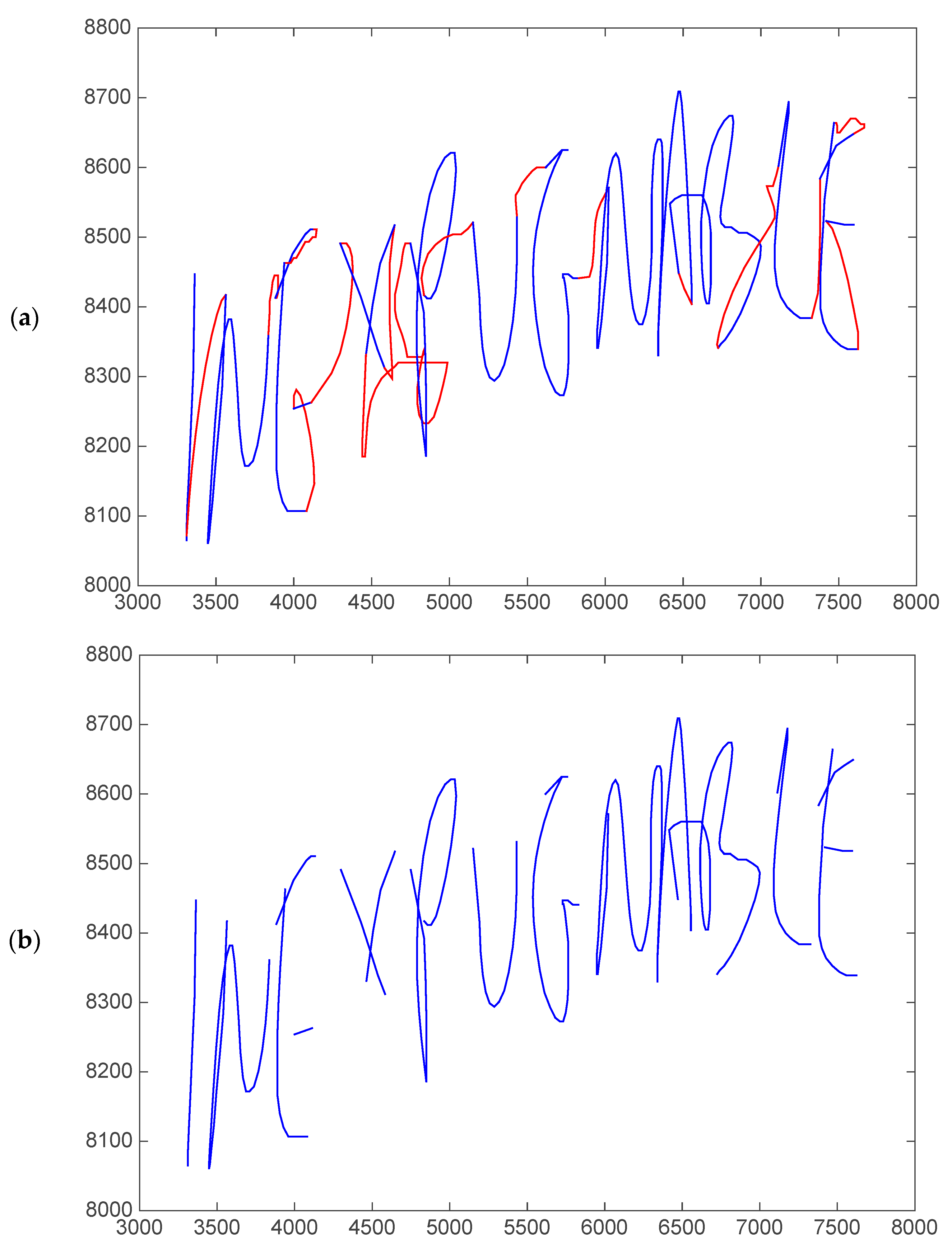
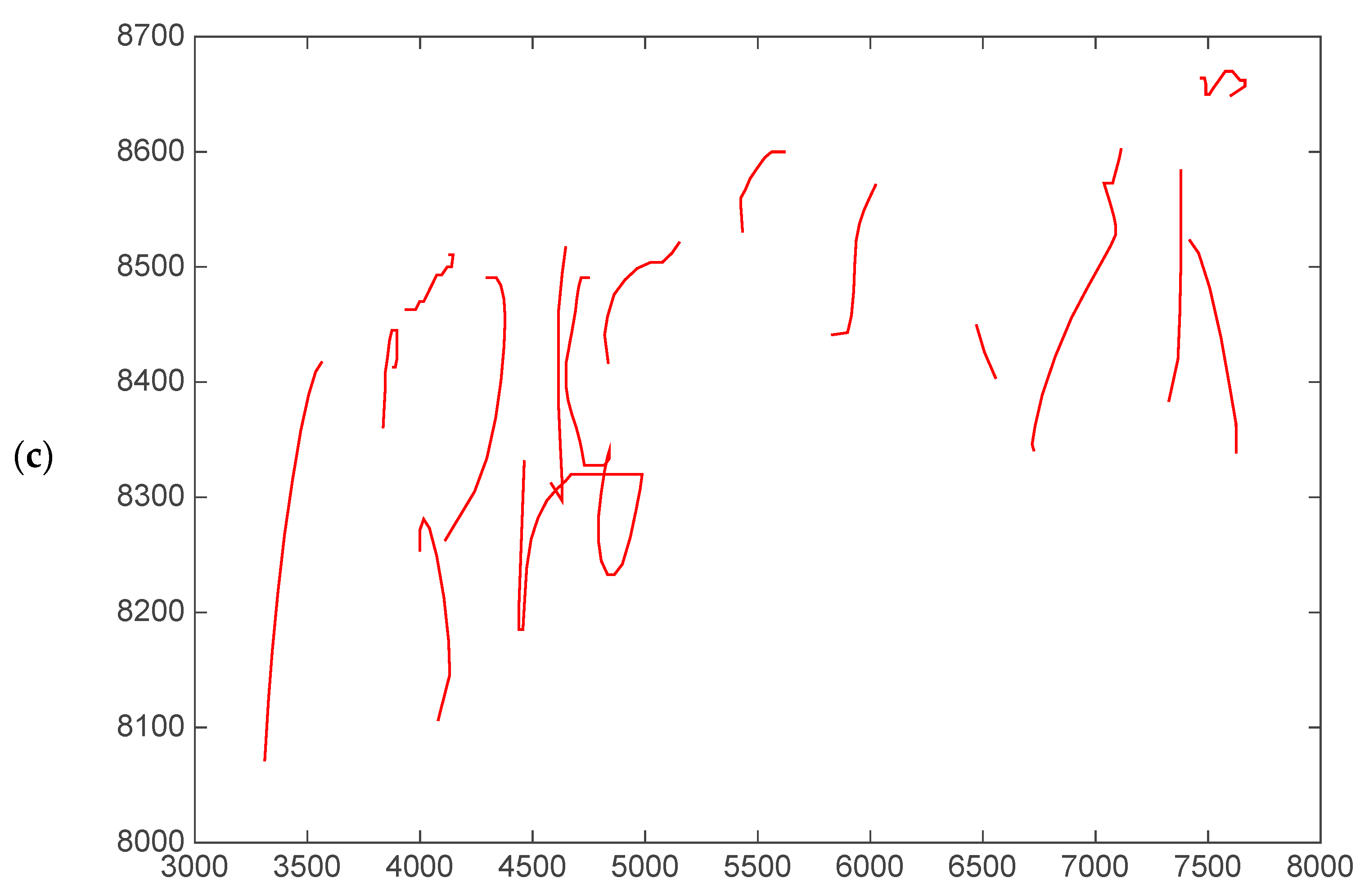
3.1. Online Drawing Applied to Health Analysis
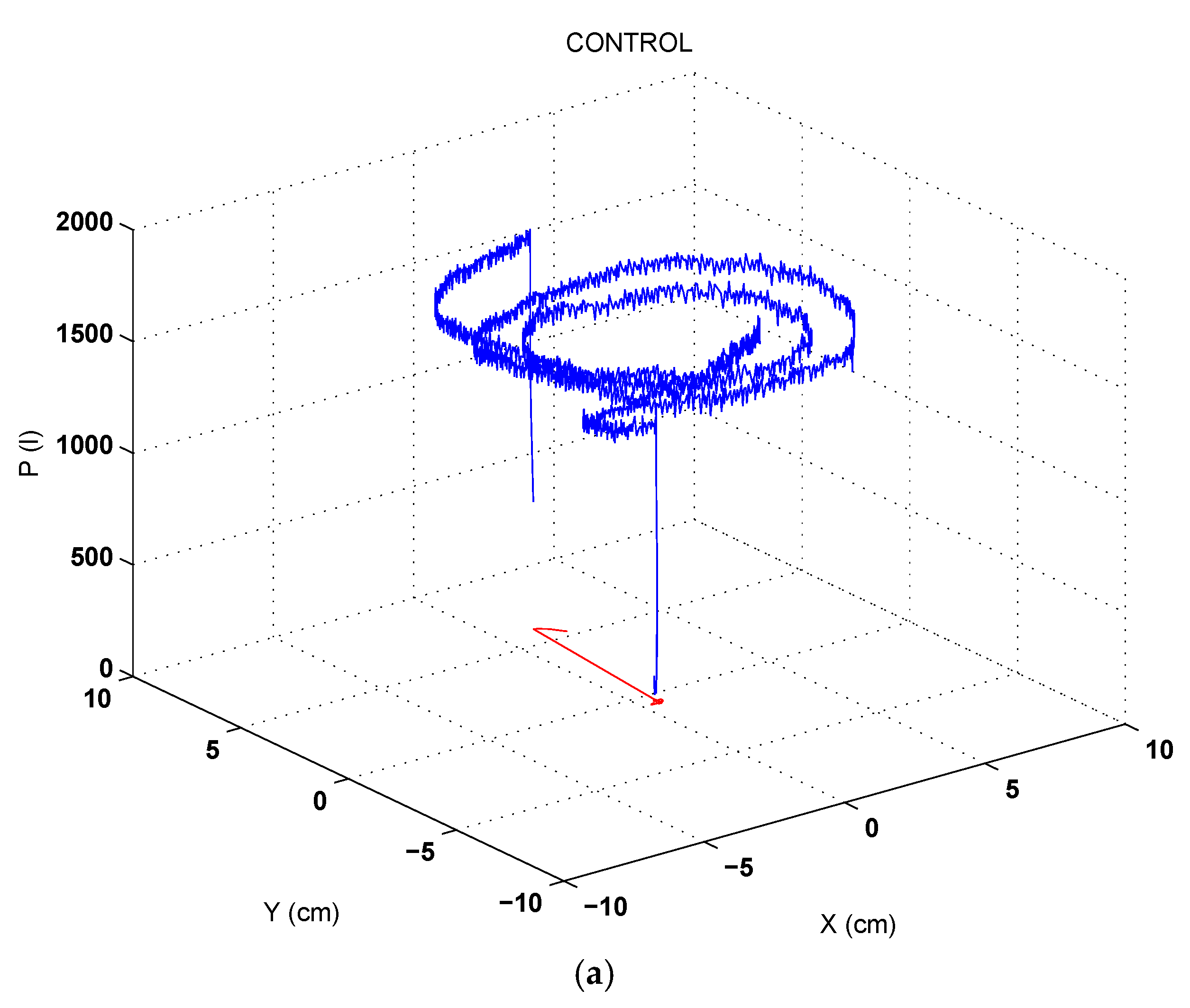
3.2. Pressure Derived Measures and in-Air Analysis
3.3. Features Extraction
3.3.1. Linear Features
- Time related measures: Time in-air, time on-surface and total time (in-air plus on-surface). Time has been measured as number of samples.
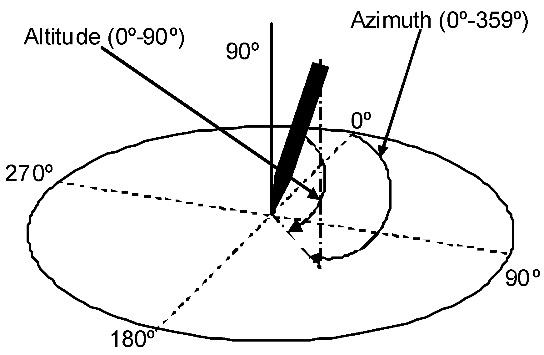
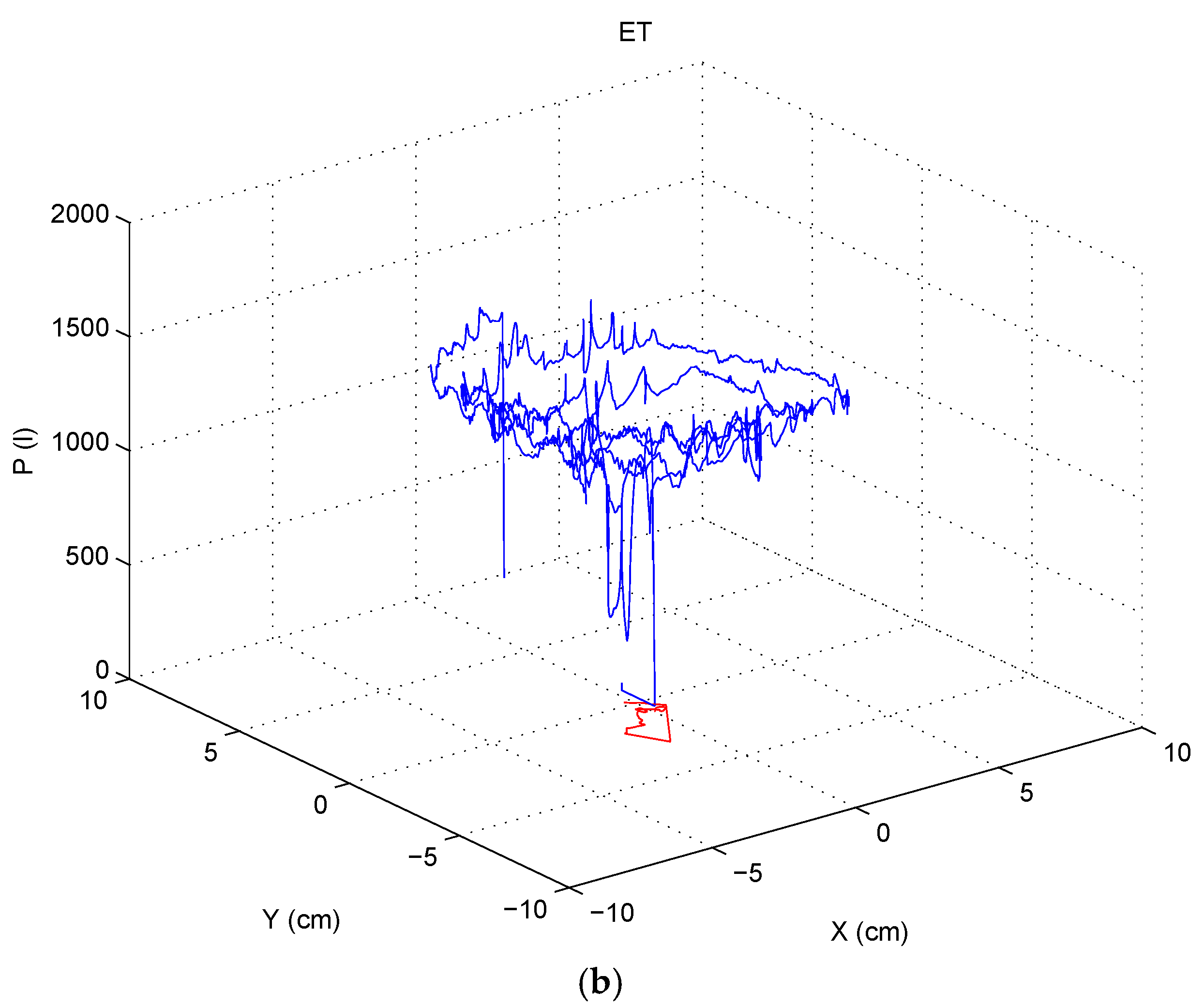
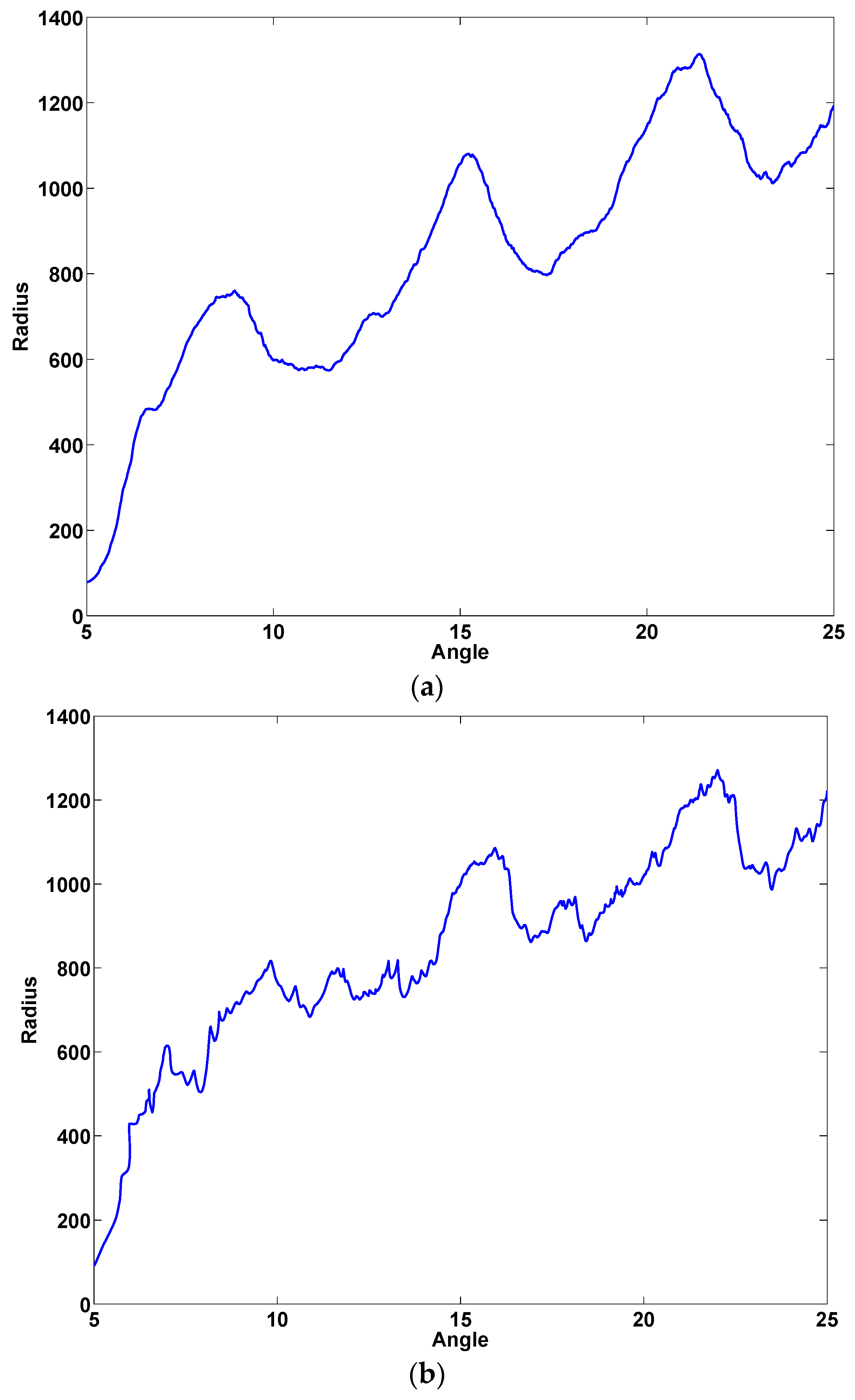
- Spatial components and their variants: and Cartesian coordinates, altitude () and azimuth () angles, and angle and modulus polar components ( and , respectively) and their projections over a horizontal axis for both pen-down and pen-up signal (see Figure 4 for an example of the distortion of the polar components in the sample of the ET patient).
- Pressure and its variants.
- Dynamic features and their variants: Speed and acceleration for both pen-down and pen-up signals.
- Zero crossing rate: The rate which evaluates the sign-changes along a signal.
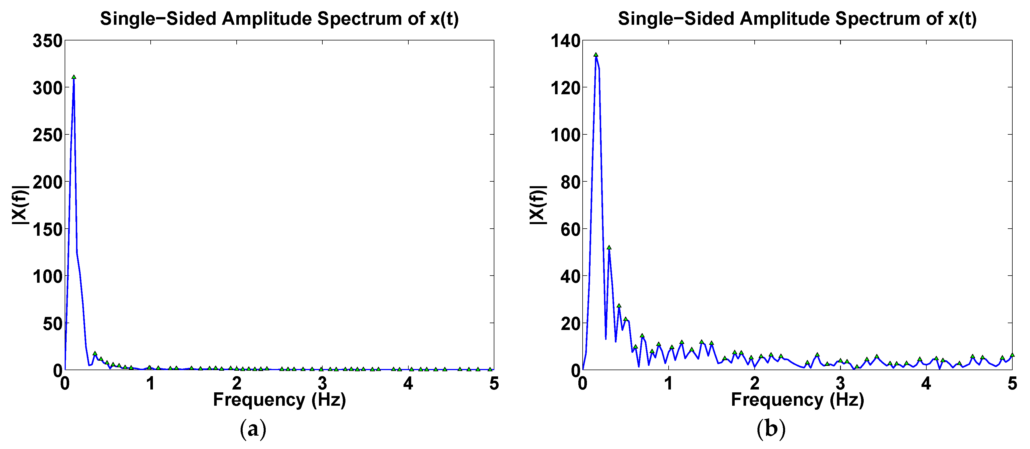
- Frequency domain: Spectral components for both pen-down and pen-up signals (Figure 5).
3.3.2. Non-Linear Features: Entropy
Shannon Entropy
Approximate Entropy versus Sample Entropy
Multivariate Multiscale Permutation Entropy
- (i)
- From the original time series, multiple successive coarse-grained versions are extracted by , where ε is the scale factor. Each element of the coarse-grained time series is calculated as:
- (ii)
- For each scaled series, the PE is calculated.
- (i)
- Different time scales of increasing length are defined by coarse-graining the original multivariate time series, i.e., {,t}, for (where is the number of channels) and for (where is number of samples in each time series). For a scale factor ε, the elements of the multivariate coarse-grained time series can be derived as:
- (ii)
- Calculate the multivariate permutation entropy, MPE, for each coarse-grained multivariate and all variants of average.
3.3.3. Feature Sets
- Linear features set (LF), the set described in Section 3.3.1
- Non-linear features sets (NLF) that consist of LF and the features described in Section 3.3.2: linear features + Shannon entropy (SE), linear features + Approximate Entropy (ApEn), linear features + Sample Entropy (SmEn) and linear features + permutation entropy (PE).
- Set after selection of features by ANOVA: selection of linear features (SLF), Selection of linear features + Shannon Entropy (SSE), Selection of linear features + Approximate Entropy (SApEn), Selection of linear features + Sample Entropy (SSmEn) and Selection of linear features + permutation entropy (SPE).
3.4. Automatic Selection of Features by ANOVA
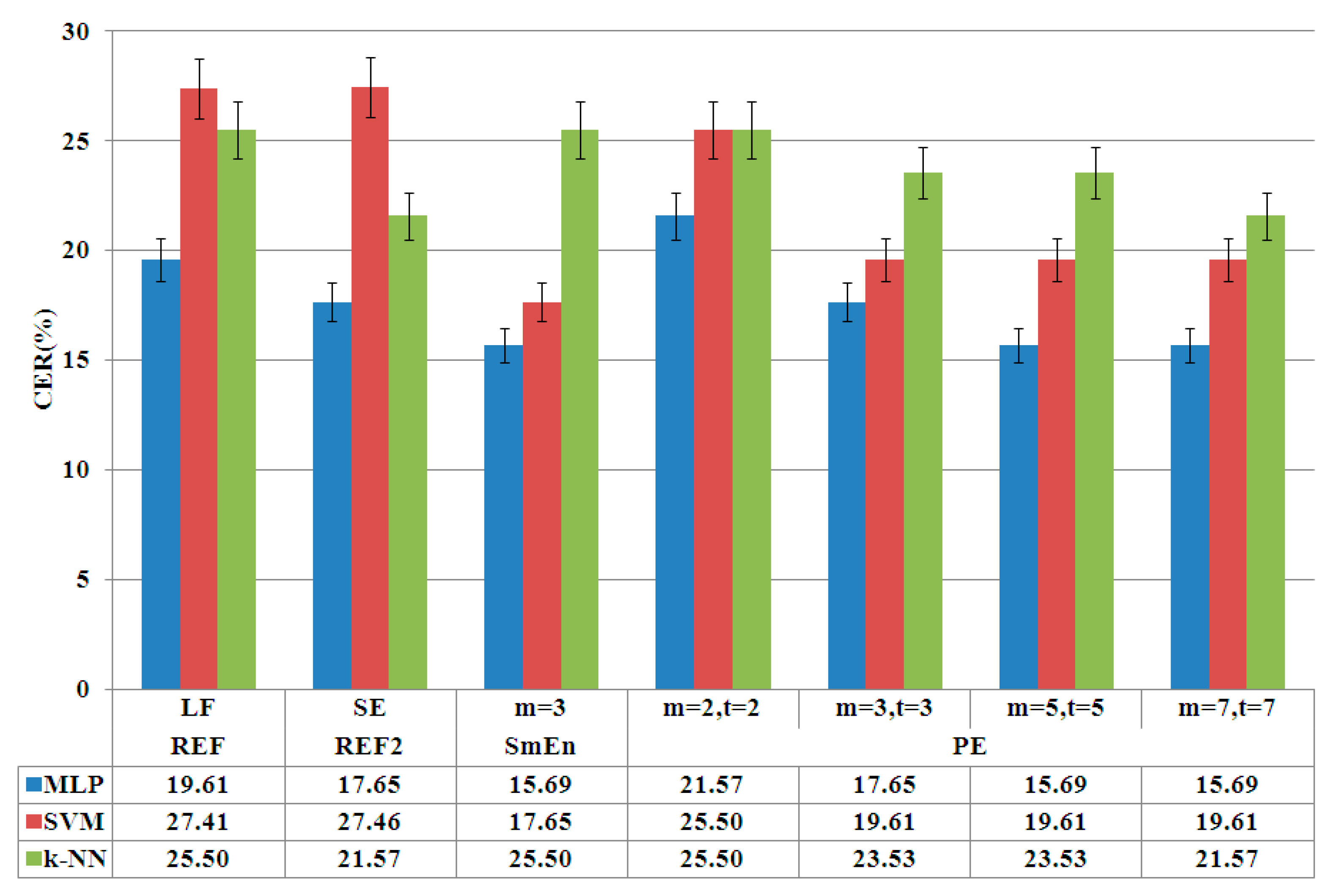
3.5. Modeling and Automatic Classification
- A Support Vector Machine (SVM) with polynomial kernel;
- A Multi Layer Perceptron (MLP) with number of units in the hidden layer given () by = max (Attribute/Number + Classes/Number) and training step (TS) = ; and
- A k Nearest Neighbor (k-NN) k-NN algorithm.
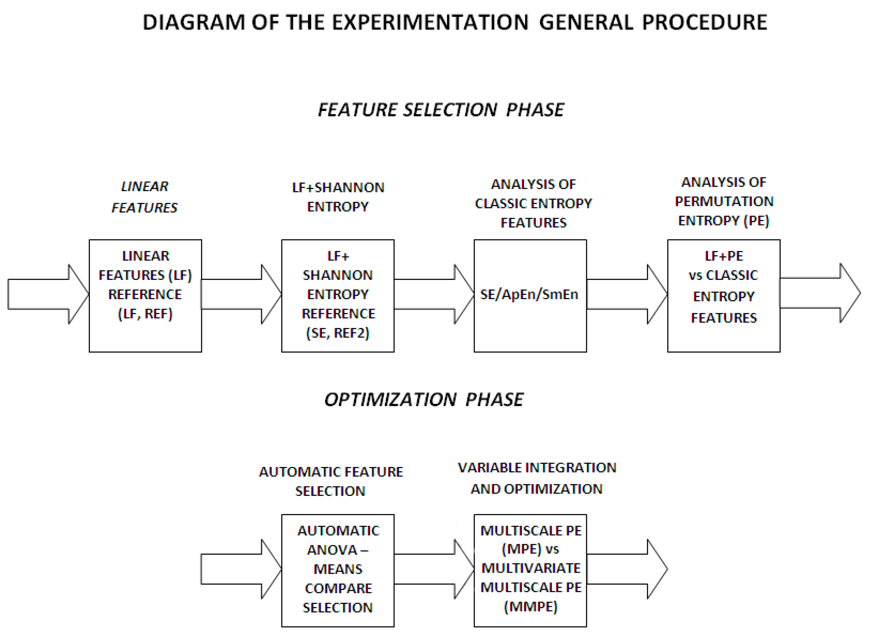
3.6. General Procedure of the Experimentation
- (1)
- Analysis of classic linear features. An automatic classification is carried out in order to obtain the reference rates (LF) for linear features.
- (2)
- Analysis of linear features and Shannon entropy. A second reference (SE) is calculated integrating linear and the classic entropy feature, Shannon entropy.
- (3)
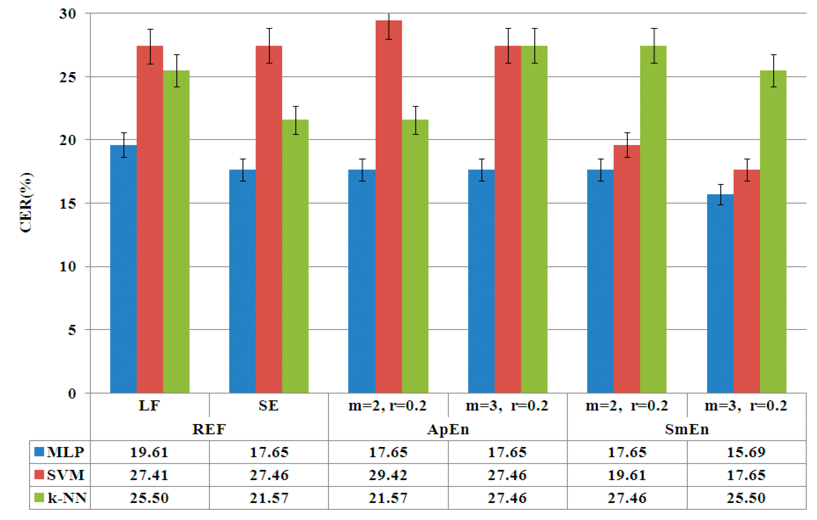
- Analysis of classic entropy features. ApEn and SmEn are analyzed and compared in order to adjust and select optimum parameters for the algorithms ( and ).
- (4)
- Entropy based classic features vs. permutation entropy. An analysis of the previous adjusted classic entropy features against permutation entropy is carried out in order to obtain the optimum parameters for permutation entropy.
- (1)
- Automatic feature selection. An automatic feature selection is carried out based on statistical-medical criteria by ANOVA and a multiple comparisons test of the group means. Thus, only the linear and non-linear features with a -value under a fixed threshold are selected and an optimum feature set is obtained.
- (2)
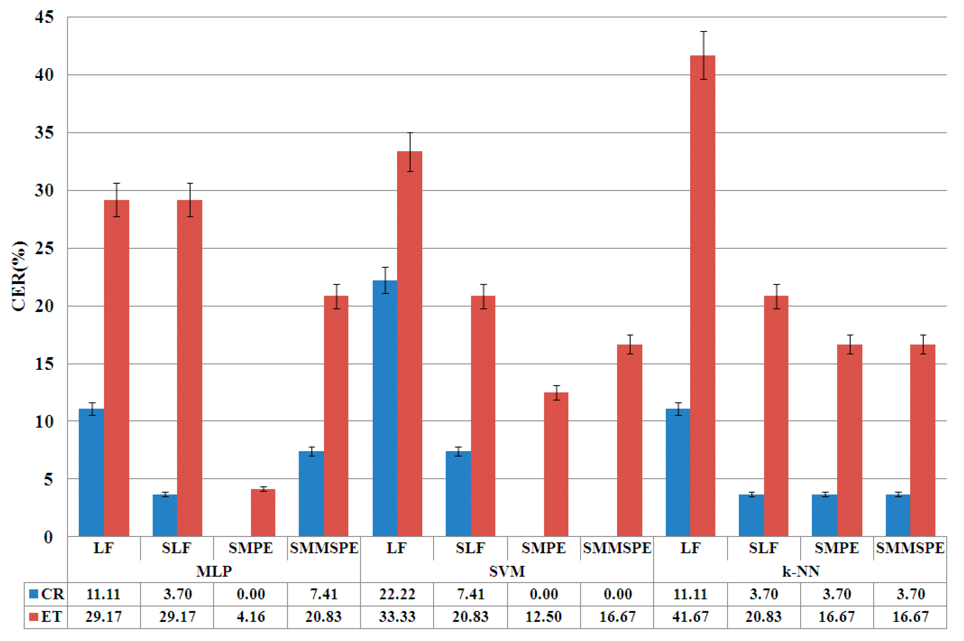
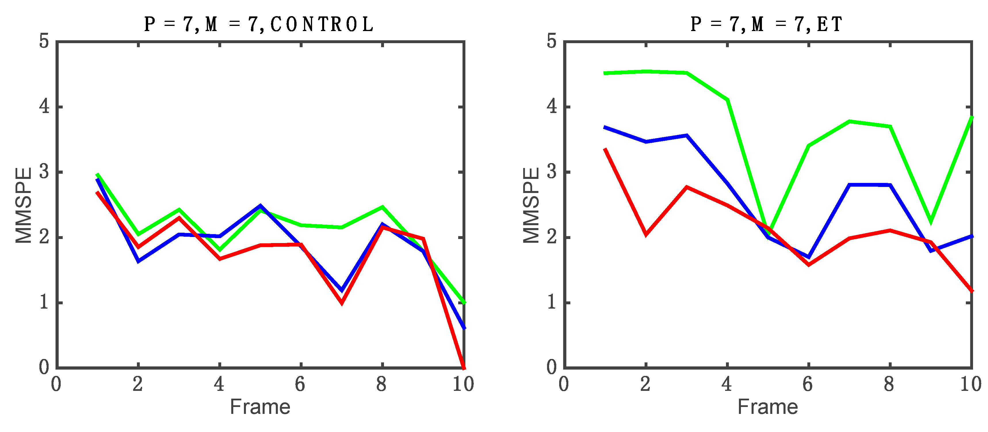
- Optimization. Finally, an optimization analysis of the PE based features is carried out. Two new algorithms are used based on: (1) scale analysis by multiscale permutation entropy (MPE); and (2) the integration of signals and scale analysis by the novel multivariate multiscale permutation entropy (MMSPE) algorithm. This last step is oriented to integrate signal correlations and to reduce even more the number of features for real-time system purposes.
4. Results and Discussion
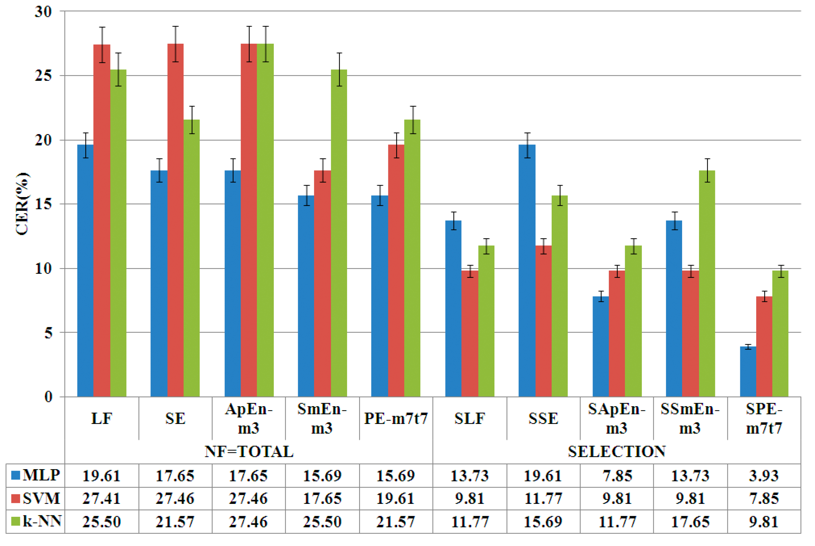
4.1. Phase of Entropy Feature Selection
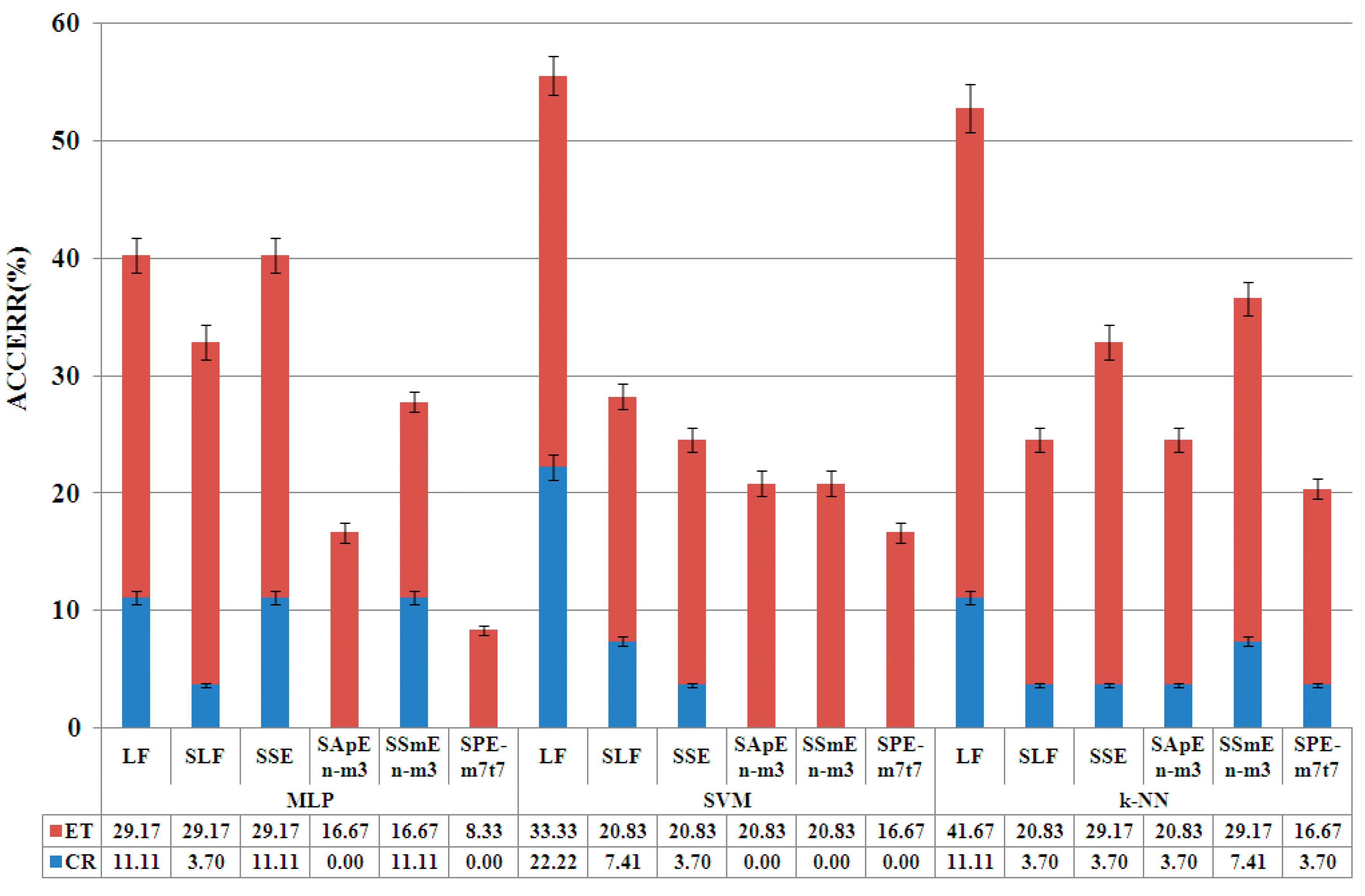
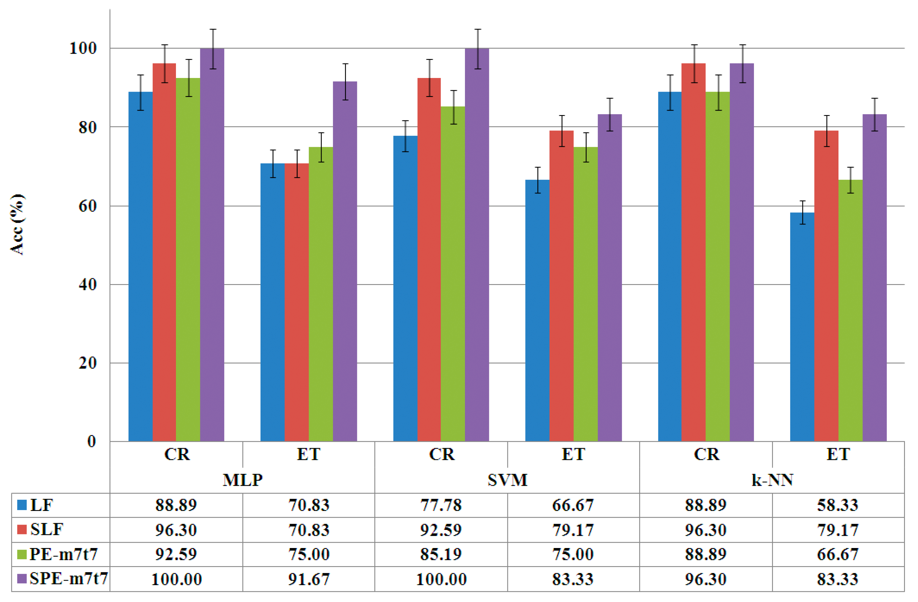
4.2. Optimization Phase
5. Conclusions
Acknowledgments
Author Contributions
Conflicts of Interest
Abbreviations
| CR | control group |
| ET | essential tremor |
| EPT | electrophysiological test |
| fMRI | functional magnetic resonance imaging |
| MoCA | Montreal Cognitive Assessment |
| EMG | electromyography |
| AD | Alzheimer’s disease |
| LF | linear features (reference) |
| SLF | selection of linear features |
| NLF | non-linear features |
| SE | linear features + Shannon entropy (reference) |
| ApEn | linear features + Approximate Entropy |
| SmEn | linear features + Sample Entropy |
| EEG | electroencephalography |
| PE | permutation entropy |
| MPE | multi scale permutation entropy |
| MSE | multiscale entropy |
| MMSE | multivariate multiscale entropy |
| MMSPE | multivariate multiscale permutation entropy |
| MLP | Multi Layer Perceptron |
| NNHL | number of hidden layers units |
| SVM | Support Vector Machine |
| CER | classification error rate |
| ACCERR | Accumulative Classification Error Rate |
| ACC | Accuracy |
| SE | linear features + Shannon entropy |
| SSE | Selection of linear features + Shannon Entropy |
| SApEn | Selection of linear features + Approximate Entropy |
| SSmEn | Selection of linear features + Sample Entropy |
| SPE | Selection of linear features + Permutation Entropy |
| SMPE | Selection of linear features + Multi scale Permutation Entropy |
| SMMSPE | Selection of linear features + Multivariate Multiscale Permutation Entropy |
References
- Zanin, M.; Zunino, L.; Rosso, O.A.; Papo, D. Permutation entropy and its main biomedical and econophysics applications: A review. Entropy 2012, 14, 1553–1577. [Google Scholar] [CrossRef]
- Morabito, F.C.; Labate, D.; La Foresta, F.; Bramanti, A.; Morabito, G.; Palamara, I. Multivariate Multi-Scale Permutation Entropy for Complexiy Analysis of Alzheimer’s Disease EEG. Entropy 2012, 14, 1186–1202. [Google Scholar] [CrossRef]
- Eguiraun, H.; López-de-Ipiña, K.; Martinez, I. Application of, Entropy and Fractal Dimension Analyses to the Pattern Recognition of Contaminated Fish Responses in Aquaculture. Entropy 2014, 16, 6133–6151. [Google Scholar] [CrossRef]
- Costa, M.; Goldberger, A.; Peng, C.K. Multiscale entropy analysis of biological signals. Phys. Rev. 2005, 71. [Google Scholar] [CrossRef] [PubMed]
- Louis, E.D.; Vonsattel, J.P. The emerging neuropathology of essential tremor. Mov. Disord. 2007, 23, 174–182. [Google Scholar] [CrossRef] [PubMed]
- Faundez-Zanuy, M.; Hussain, A.; Mekyska, J.; Sesa-Nogueras, E.; Monte-Moreno, E.; Esposito, A.; Chetouani, M.; Garre-Olmo, J.; Abel, A.; Smekal, Z.; et al. Biometric Applications Related to Human Beings: There Is Life beyond Security. Cogn. Comput. 2013, 5, 136–151. [Google Scholar] [CrossRef]
- López-de-Ipiña, K.; Alonso, J.B.; Solé-Casals, J.; Barroso, N.; Faundez-Zanuy, M.; Travieso, C.; Ecay-Torres, M.; Martinez-Lage, P.; Martinez-de-Lizardui, U. On the selection of non-invasive methods based on speech analysis oriented to Automatic Alzheimer Disease Diagnosis. Sensors 2013, 13, 6730–6745. [Google Scholar] [CrossRef] [PubMed] [Green Version]
- Laske, C.; Sohrabi, H.R.; Frost, S.M.; López-de-Ipiña, K.; Garrard, P.; Buscem, M.; Dauwels, J.; Soekadar, S.R.; Mueller, S.; Linnemann, C.; et al. Innovative diagnostic tools for early detection of Alzheimer’s disease. Alzheimer Dement. 2015, 11, 561–578. [Google Scholar] [CrossRef] [PubMed]
- Sesa-Nogueras, E.; Faundez-Zanuy, M. Biometric recognition using online uppercase handwritten text. Pattern Recognit. 2012, 45, 128–144. [Google Scholar] [CrossRef]
- Pullman, S.L. Spiral Analysis: A New Technique for Measuring Tremor with a Digitizing Tablet. Mov. Disord. 1998, 13, 85–89. [Google Scholar] [CrossRef] [PubMed]
- WACOM. Available online: http://www.wacom.com (accessed on 10 May 2016).
- Faundez-Zanuy, M. Online signature recognition based on VQ-DTW. J. Pattern Recognit. 2007, 40, 981–982. [Google Scholar] [CrossRef]
- López-de-Ipiña, K.; Bergareche, A.; De La Riva, P.; Faundez-Zanuy, M.; Calvo, P.M.; Roure, J.; Sesa-Nogueras, E. Automatic non-linear analysis of non-invasive writing signals, applied to essential tremor. J. Appl. Log. 2015. [Google Scholar] [CrossRef]
- López-de-Ipiña, K.; Iturrate, M.; Calvo, P.M.; Beitia, B.; Garcia-Melero, J.; Bergareche, A.; De La Riva, P.; Marti-Masso, J.F.; Faundez-Zanuy, M.; Sesa-Nogueras, E.; et al. Selection of Entropy Based Features for the Analysis of the Archimedes’ Spiral Applied to Essential Tremor. In Proceedings of the 4th IEEE International Work Conference on Bioinspired, Intelligence, Donostia, Spain, 9–12 June 2015; pp. 157–162.
- Ortega-Garcia, J.; Gonzalez-Rodriguez, J.; Simon-Zorita, D.; Cruz-Llanas, S. From Biometrics Technology to Applications Regarding Face, Voice, Signature and Fingerprint Recognition Systems. In Biometric Solutions for Authentication in an E-World; Kluwer Academic Publishers: Berlin, Germany, 2002; pp. 289–337. [Google Scholar]
- The Montreal Cognitive Assessment (MoCA). Available online: http://www.mocatest.org/ (accessed on 10 May 2016).
- Faundez-Zanuy, M.; Sesa-Nogueras, E.; Roure-Alcobé, J.; Garré-Olmo, J.; López-de-Ipiña, K.; Solé-Casals, K. Online Drawings for Dementia Diagnose: In-Air and Pressure Information Analysis. In XIII Mediterranean Conference on Medical and Biological Engineering and Computing; Springer International Publishing: New York, NY, USA, 2014; pp. 567–570. [Google Scholar]
- Neils-Strunjas, J.; Groves-Wright, K.; Mashima, P.; Harnish, S. Dysgraphia in Alzheimer’s disease: A review for clinical and research purposes. J. Speech Lang. Hear. Res. 2006, 49, 1313–1330. [Google Scholar] [CrossRef]
- Phillips, J.G.; Ogeil, R.P.; Müller, F. Alcohol consumption and handwriting: A kinematic analysis. Hum. Mov. Sci. 2009, 28, 619–632. [Google Scholar] [CrossRef] [PubMed]
- Foley, R.G.; Miller, A.L. The effects of marijuana and alcohol usage on handwriting. Forensic Sci. Int. 1979, 14, 159–164. [Google Scholar] [CrossRef]
- Tucha, O.; Walitza, S.; Mecklinger, L.; Stasik, D.; Sontag, T.; Lange, K.W. The effect of caffeine on handwriting movements in skilled writers. Hum. Mov. Sci. 2006, 25, 523–535. [Google Scholar] [CrossRef] [PubMed]
- Rosenblum, S.; Parush, S.; Weiss, P.L. The in Air Phenomenon: Temporal and Spatial Correlates of the Handwriting Process. Percept. Mot. Skills 2003, 96, 933–954. [Google Scholar] [CrossRef] [PubMed]
- Sadikov, A.; Groznik, V.; Žabkar, J.; Mozina, M.; Georgiev, D.; Pirtosek, Z.; Bratko, I. Parkinson Check smart phone app. In Frontiers in Artificial Intelligence and Applications; IOS Press: Amsterdam, The Netherlands, 2014; Volume 263, pp. 1213–1214. [Google Scholar]
- Georgiev, D.; Groznik, V.; Sadikov, A.; Mozina, M.; Guid, M.; Kragelj, V.; Bratko, I.; Ribaric, S.; Pirtosek, Z. Digitalised spirography and clinical examination based decision support system of differentiating between tremors. Eur. J. Neurol. 2012, 19, 298. [Google Scholar]
- Bolle, R.; Pankanti, S. Biometrics, Personal Identification in Networked Society; Jain, A., Ed.; Kluwer Academic Publishers: Norwell, MA, USA, 1998. [Google Scholar]
- Faundez-Zanuy, M. Privacy issues on biometric systems. In IEEE Aerospace and Electronic Systems Magazine; IEEE Xplore: New York, NY, USA, 2005; Volume 20, pp. 13–15. [Google Scholar]
- Gray, R.M. Entropy and Information Theory; Springer: Berlin/Heidelberg, Germany, 1990. [Google Scholar]
- Brissaud, J.B. The meaning of entropy. Entropy 2005, 7, 68–96. [Google Scholar] [CrossRef]
- Shannon, C.E. A mathematical theory of communication. Bell Syst. Tech. J. 1948, 27, 379–423. [Google Scholar] [CrossRef]
- Shannon, C.E.; Weaver, W. The Mathematical Theory of Communication; University of Illinois Press: Champaign, IL, USA, 1949. [Google Scholar]
- Richman, J.S.; Moorman, J.R. Physiological time-series analysis using approximate entropy and sample entropy. Am. J. Physiol. Heart Circ. Physiol. 2000, 278, 2039–2049. [Google Scholar]
- Pincus, S.M.; Huang, W.M. Approximate entropy, statistical properties and applications. Commun. Stat. Theory Methods 1992, 21, 3061–3077. [Google Scholar] [CrossRef]
- Pincus, S.M. Approximate entropy as a measure of system complexity. Proc. Natl. Acad. Sci. USA 1991, 88, 2297–2301. [Google Scholar] [CrossRef] [PubMed]
- Dragomir, A.; Akay, Y.; Curran, A.K. Investigating the complexity of respiratory patterns during the laryngeal chemoreflex. J. NeuroEng. Rehabil. 2008, 5. [Google Scholar] [CrossRef] [PubMed]
- Yentes, J.M.; Hunt, N.; Schmid, K.; Kaipust, J.P.; McGrath, D.; Stergiou, N. The use of approximate entropy and sample entropy with short data sets. Ann. Biomed. Eng. 2013, 41, 349–365. [Google Scholar] [CrossRef] [PubMed]
- Ramanand, P.; Nampoori, V.P.; Sreenivasan, R. Complexity quantification of dense array EEG using sample entropy analysis. J. Integr. Neurosci. 2004, 3, 343–358. [Google Scholar] [CrossRef] [PubMed]
- Solé-Casals, J.; Vialatte, F.B. Towards Semi-Automatic Artifact Rejection for the Improvement of Alzheimer’s Disease Screening from EEG Signals. Sensors 2015, 15, 17963–17976. [Google Scholar] [CrossRef] [PubMed]
- Bandt, C.; Pompe, B. Permutation entropy: A natural complexity measure for time series. Phys. Rev. Lett. 2002, 88. [Google Scholar] [CrossRef] [PubMed]
- Keller, K.; Lauffer, H. Symbolic analysis of high-dimensional time series. Int. J. Bifurc. Chaos 2003, 13, 2657–2668. [Google Scholar] [CrossRef]
- Ahmed, M.U.; Mandic, D.P. Multivariate multiscale entropy. In IEEE Signal Processing Letters; IEEE Xplore: New York, NY, USA, 2012; Volume 19, pp. 91–95. [Google Scholar]
- Mathworks. Available online: http://www.mathworks.com (accessed on 10 May 2016).
- Weka. Available online: http://www.cs.waikato.ac.nz/ml/weka (accessed on 10 May 2016).
- Picard, R.; Cook, D. Cross-Validation of Regression Models. J. Am. Stat. Assoc. 1984, 79, 575–583. [Google Scholar] [CrossRef]
- Witten, I.H.; Frank, E. Data Mining: Practical Machine Learning Tools and Techniques, 2nd ed.; Morgan Kaufmann: San Francisco, CA, USA, 2005. [Google Scholar]


| ET_X | EPT Features | Diagnosis | Demography | |||
|---|---|---|---|---|---|---|
| Frequency (Hz) | Amplitude (v) | Pattern | FTM Scale | Age | Gender | |
| ET_01 | 8.5 | 20 | synchronous | 1 | 48 | Female |
| ET_02 | 6.5 | variable | alternating | 8 | 72 | Male |
| ET_03 | 10.5 | 200 | synchronous | 1 | 46 | Male |
| ET_04 | 4.5 | 503.6 | synchronous | 3 | 80 | Female |
| ET_05 | 6.6 | 298 | synchronous | 22 | 68 | Female |
| ET_06 | 9.5 | 46 | synchronous | 2 | 46 | Female |
| ET_07 | 5 | 173 | synchronous | 50 | 75 | Male |
| ET_08 | 6.5 | 159 | synchronous | 40 | 75 | Male |
| ET_09 | 8 | 128 | asynchronous | 9 | 75 | Female |
| LF | SE | ApEn-m3 | SmEn-m3 | PE-m7t7 | SLF | SSE | SApEn-m3 | SSmEn-m3 | SPE-m7t7 | |
|---|---|---|---|---|---|---|---|---|---|---|
| FN | 186 | 198 | 198 | 198 | 198 | 70 | 76 | 73 | 77 | 78 |
| MLP | SVM | k-NN | |
|---|---|---|---|
| LF | 19.61 | 27.41 | 25.50 |
| SLF | 13.73 | 9.81 | 11.77 |
| SPE-m7t7 | 3.93 | 7.85 | 9.81 |
© 2016 by the authors; licensee MDPI, Basel, Switzerland. This article is an open access article distributed under the terms and conditions of the Creative Commons Attribution (CC-BY) license (http://creativecommons.org/licenses/by/4.0/).
Share and Cite
López-de-Ipiña, K.; Solé-Casals, J.; Faundez-Zanuy, M.; Calvo, P.M.; Sesa, E.; Martinez de Lizarduy, U.; De La Riva, P.; Marti-Masso, J.F.; Beitia, B.; Bergareche, A. Selection of Entropy Based Features for Automatic Analysis of Essential Tremor. Entropy 2016, 18, 184. https://doi.org/10.3390/e18050184
López-de-Ipiña K, Solé-Casals J, Faundez-Zanuy M, Calvo PM, Sesa E, Martinez de Lizarduy U, De La Riva P, Marti-Masso JF, Beitia B, Bergareche A. Selection of Entropy Based Features for Automatic Analysis of Essential Tremor. Entropy. 2016; 18(5):184. https://doi.org/10.3390/e18050184
Chicago/Turabian StyleLópez-de-Ipiña, Karmele, Jordi Solé-Casals, Marcos Faundez-Zanuy, Pilar M. Calvo, Enric Sesa, Unai Martinez de Lizarduy, Patricia De La Riva, Jose F. Marti-Masso, Blanca Beitia, and Alberto Bergareche. 2016. "Selection of Entropy Based Features for Automatic Analysis of Essential Tremor" Entropy 18, no. 5: 184. https://doi.org/10.3390/e18050184