Training Concept, Evolution Time, and the Maximum Entropy Production Principle

Abstract

The maximum entropy production principle (MEPP) is a type of entropy optimization which demands that complex non-equilibrium systems should organize such that the rate of the entropy production is maximized. Our take on this principle is that to prove or disprove the validity of the MEPP and to test the scope of its applicability, it is necessary to conduct experiments in which the entropy produced per unit time is measured with a high precision. Thus we study electric-field-induced self-assembly in suspensions of carbon nanotubes and realize precise measurements of the entropy production rate (EPR). As a strong voltage is applied the suspended nanotubes merge together into a conducting cloud which produces Joule heat and, correspondingly, produces entropy. We introduce two types of EPR, which have qualitatively different significance: global EPR (g-EPR) and the entropy production rate of the dissipative cloud itself (DC-EPR). The following results are obtained: (1) As the system reaches the maximum of the DC-EPR, it becomes stable because the applied voltage acts as a stabilizing thermodynamic potential; (2) We discover metastable states characterized by high, near-maximum values of the DC-EPR. Under certain conditions, such efficient entropy-producing regimes can only be achieved if the system is allowed to initially evolve under mildly non-equilibrium conditions, namely at a reduced voltage; (3) Without such a “training” period the system typically is not able to reach the allowed maximum of the DC-EPR if the bias is high; (4) We observe that the DC-EPR maximum is achieved within a time, T_e, the evolution time, which scales as a power-law function of the applied voltage; (5) Finally, we present a clear example in which the g-EPR theoretical maximum can never be achieved. Yet, under a wide range of conditions, the system can self-organize and achieve a dissipative regime in which the DC-EPR equals its theoretical maximum.

1. Introduction

Nature appears to be ordered in multiple ways and at various levels, seemingly contradicting the second law of thermodynamics, which demands the maximum disorder. Moreover, it seems that in Nature the order increases over time, as exemplified by the occurrence and the evolution of the life on Earth. Apparently, life is initiated and maintained by the ordering effect of the Sun. Technically speaking, the Sun provides us with a flow of high energy photons, which, due to their relatively high temperature, as compared to the cosmic background, as well as due to their non-equilibrium frequency distribution as they arrive to Earth, represent a state with a large free energy and with a strongly reduced entropy. Thus the sunlight has an ordering effect and can thus initiate and sustain biological life.

On the other hand, it appears that many living organisms, which represent a highly organized state with a reduced entropy, can be viewed as systems which are efficient in harvesting free energy deposited by the sunlight and efficient in generating entropy. Such a view on life has been discussed by Schrödinger [1]. For examples, plants are good at capturing photons and producing sugar, and animals are good at eating this sugar and generating heat, i.e., these biological systems seem to contribute to the entropy production. Any self-organized system occurring far from equilibrium can be characterized quantitatively by the increase of its entropy per unit time, i.e., by its entropy production rate (EPR) [2,3].

The central question is this: if a source of free energy is present, should a complex system, which is able to intercept the free energy flow, self-organize to the extent that the EPR is always maximized? Another big question is stated in [2], namely to understand the reasons why the life continuously develops and becomes more and more complex (a possible answer is suggested in Section 10). And is it possible to answer this question within the scope of thermodynamics? A significant progress in the understanding of such important question is only possible if rigorous experiments are performed, in parallel with the advancement of theory. Yet, as the far as we know, experimental investigations of the entropy generation rate in systems far from equilibrium are lacking. This fact gives us a strong motivation to study experimentally model systems which can be understood in terms of the entropy production rate.

Here we present experiments which indicate that in some cases the most efficient regime, i.e., the regime corresponding to the DC-EPR maximum, is much more stable than all other stages of the system evolution. We have also observed cases in which the system can achieve its DC-EPR maximum if it is introduced to the metastable regime through a particular process, termed “training”, which is essentially an evolution under mildly non-equilibrium conditions. If such training is not provided then its DC-EPR, as well as g-EPR, remain much lower than their maximum allowed values, at all times. Here and everywhere we use the notation of DC-EPR to refer to the entropy production by the dissipative cloud itself, while g-EPR refers to the entropy production by the entire system, including the source and the load. Let us clarify once again that the DC-EPR is the amount of heat generated within the self-assembled cloud per unit time divided by the temperature of the environment.

The global entropy production rate, g-EPR, is the amount of heat generated in the entire circuit per unit time, divided by the temperature of the environment. Thus DC-EPR is the entropy production rate caused by the dissipative cloud and the g-EPR is the entropy production rate caused by the dissipative cloud and the source of the free energy taken together. We argue and confirm experimentally that g-EPR cannot be achieved, at least in the systems analogous to our system with limited dissipation.

We also present evidence that the evolution time, needed to achieve the DC-EPR maximum, scales approximately as a power law with the applied thermodynamic potential (the voltage). And, to achieve the DC-EPR maximum, the conditions should be within some acceptable range. To obtain these results we study a system in which the maximum values of the DC-EPR and the g-EPR are both well-defined and can be easily calculated as well as accurately measured.

2. Historical Remarks on MEPP

Maximum entropy production principle (MEPP) has been discussed by many authors. Some of the earlier works belong to Onsager [4,5], Ziegler [6,7], Swenson and Turvey [8,9]. According to the MEPP, a non-equilibrium system evolves such as to maximize its EPR under the present constraints [8,9]. Thus MEPP has been suggested by some authors as a hypothetical new law of Nature, which might be needed to explain climate patterns [10,11,12], biological systems [13,14], and physical problems [15,16,17,18]. A modeling of electric discharge with entropy production rate has been published by Christen [19]. More details about the MEPP can be found in recent review articles [20,21,22]. Different versions of the MEPP have been considered previously [4,5,6,7]. Some authors argued that the MEPP is not true [23,24,25,26,27,28]. However, according to Martyushev and Seleznev [21,29] all these claims refer to experiments which violate, in one way or another, some applicability conditions of the principle. To further clarify the subject we need more experiments on systems in which: (1) the EPR can be measured with a high precision and (2) the maximum possible EPR is known precisely. Below we present a brief overview of what has been done and suggest what should be studied next.

It is well known that complex systems (i.e., systems containing a macroscopic number of interacting particles) frequently show some ordering or patterns [30]. A spontaneous self-assembly has been studied in systems of particles dispersed in colloids [31,32,33]. Particles suspended at air-fluid interfaces [34,35] as well as at a fluid-fluid interfaces [36] can also present an orderly behavior.

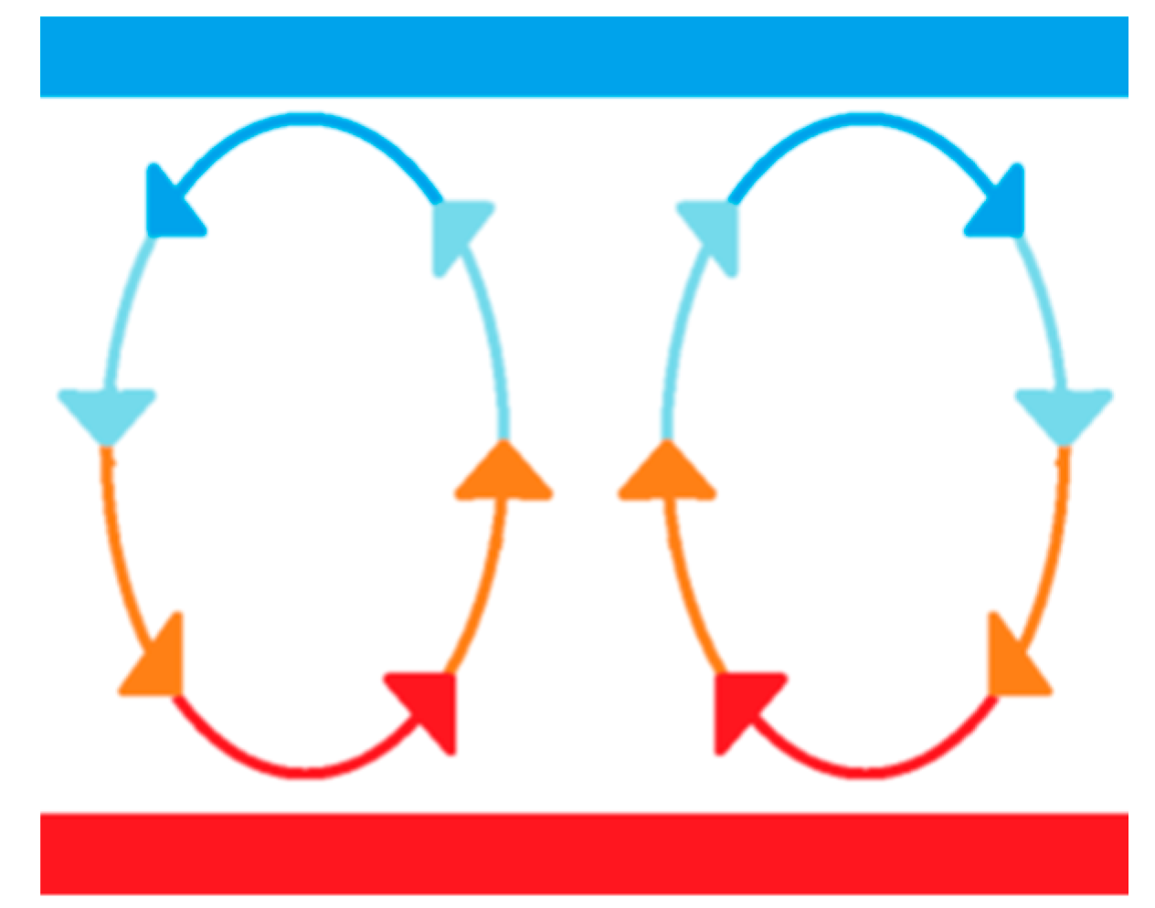
One of the best-known examples of an ordering phenomenon, which leads to a drastic increase of the EPR, is the self-organization of a heated fluid into so-called Rayleigh–Bénard (RB) convection cells [37]. The RB convection cells occur if a plane horizontal layer of a viscous fluid (e.g., oil) is placed on a hot plate, and the fluid is heated from below (Figure 1).

It appears as though the heated oil in the Bénard cell experiments becomes somewhat “intelligent”: A pattern of convection cells occurs since in this case the hot fluid from the bottom and the cold fluid from the top can move without mutual interference, in a spatially separated region. Thus the free energy is consumed faster and the entropy production is increased due to the RB convection. In this example the equilibrium state is the state in which the hot plate cools down to the temperature of the cold reservoir. The entropy production in the RB experiment is defined by the amount of heat transferred from the hot plate to the cold reservoir per unit time, dQ/dt. The formula is well known from the elementary thermodynamics, namely dS/dt = (dQ/dt)(1/T_c − 1/T_h) where T_h is the temperature of the bottom hot plate and T_c is the temperature of the top cold reservoir. What appears to be not well understood is the question on whether the occurrence of the RB convection allows the system to achieve the maximum possible value of the EPR or it does not. Of course the question is not a very easy one because one can just say that whatever value of EPR is achieved that value should be taken as the maximum possible value. In such interpretation MEPP is always correct but it does not have any predictive value. To make the hypothetical principle scientifically valuable and to prove it, two key conditions have to be satisfied: (1) There should be an independent way to determine the maximum rate of the entropy production for the given constraints. This can be achieved by a theoretical evaluation of the system considered, or by some independent experiment; (2) There should be a method to measure precisely the entropy produced per unit time, in order to compare to the expected and the actual entropy production rates. It seems that so far such conditions have not been realized in many case. Here we propose a model system which allows such evaluations.

Here we study a system where the EPR can be measured precisely, because it is defined by an electric current in the circuit, and it is a rather straightforward task to measure the electric current. The system studied is a suspension of electrically conducting carbon nanotubes biased with a high voltage. The entropy generated in a unit of time is defined by the Joule heating power. The interesting feature of the system is the existence of quasi-stable dynamic regimes, some of which have a high value of EPR and some are low. Thus the system does not always end up in the dynamic regime in which the entropy production is the highest possible. The advantage of our model system is that the maximum value of EPR is well defined and it can be simply calculated, which will be discussed in detail later in the paper.

3. Maximum Entropy Production Principle and Our Main Findings

As Hill stated [38], it seems plausible that if the total entropy of the system and its environment must approach the maximum (according to the second law of thermodynamics) then it should do so as fast as possible. This statement is equivalent to saying that the entropy should be produced by the system at a maximum possible rate. The main questions are: (1) how to formulate this statement mathematically; and (2) how to prove this hypothesis experimentally.

Swenson and Turvey conjectured that the maximum entropy production principle should be viewed as a physical selection principle. They explain that “thermodynamic fields will behave in such a fashion as to get to the final state—minimize the field potential or maximize the entropy—at the fastest possible rate given the constraints”. To prove or disprove this MEPP formulation one needs an independent way to determine what value of the EPR corresponds to its maximum. And how to define the constraints mathematically is not well established. We need to be able to determine somehow the value of the fastest possible rate of the entropy maximization, for a given system with all its constraints. This seems to be a very complicated task, unless a simple model system is selected [39].

We study experimentally a model system with a limited dissipation power. The main constraint in this system is that, no matter how much organization is achieved in the system, the heat power is always less than a certain finite value (we will see later that this value is V²/R_s for the whole system and V²/(4R_s) for the fluid with nanotubes). Of course, in any realistic system the EPR must be limited. So such a feature of our model system is useful and realistic. In our system the EPR can be computed if the current or the resistance of the fluid with nanotubes are known. In fact the EPR equals the Joule heating power divided by the temperature of the environment. Our consideration is limited to the cases where the temperature variations are negligible. The current is measured with a high precision apparatus. Thus, the Joule heating power and the entropy production rate can be determined experimentally. Therefore an experimental verification of the MEPP is achieved here.

Our experiments suggest that there are some limitations to the MEPP. In many situations, the MEPP appears to have a probabilistic nature, not a deterministic one. In other words, thermodynamic systems far from equilibrium are not always able to maximize its EPR. In certain situations the state in which DC-EPR is a maximum or near its maximum is a quasi-stable one, while the state in which the DC-EPR is very low compared to the maximum is a quasi-stable also. In what follows we investigate the limiting factors to the applicability of the MEPP, observed on carbon nanotube suspensions.

The first limiting factor to the hypothesis that EPR is always at its maximum is the obvious idea that it takes time for the system to organize from a completely disordered configuration. Note that our underlying assumption is that the system initially is disordered, then a strong thermodynamic potential is applied and the system begins to self-organize to minimize this potential. Furthermore, disordered configurations usually cannot generate as much entropy as the ordered ones. Thus it is plausible that EPR might not be able to achieve its theoretically possible maximum at the beginning of the evolution of the dissipative structure. Our tests show that the evolution time scales with the applied potential approximately as a power law.

The second limiting factor is presence of metastable states. Consider first an obvious example, a forest fire. Let us assume that if the fire is active then EPR is at its maximum. But the fire could be extinguished, or it could never start in the first place if there is no triggering event such as, e.g., a lightning strike. Therefore, if there is no fire, the entropy would be produced at a much lower rate. Thus, although the state with a high EPR (the fire) is an allowed state, it is not true to say that such state is always realized, within a finite time of observation (although, in the limit of infinite time, it might be true that the fire would always happen, sooner or later). Therefore EPR might not always be at its maximum. This appears to be in contradiction to the theoretical proposals requiring that EPR must always be maximized.

Here we observe that for a high-EPR metastable state to occur the system should be allowed to undergo some initial evolution at a relatively low potential. This gives it a chance to organize and achieve the maximum DC-EPR at a given low potential. We call this initial evolution as the “training” period. Then, as the potential is increased, the system is ready for this and it remains in the high EPR regime even at a high bias, for a seemingly indefinitely long times. Yet, if the applied potential is high from the very beginning then the high-EPR regime is never achieved, although it is not forbidden by the existing constraints, as is demonstrated experimentally by observing the high-EPR dissipative cloud at the same high potential, but after a “training session” was provided.

The third limiting factor is that the thermodynamic potential driving the self-assembly should not be too high or too low for the DC-EPR to approach its theoretical maximum. Otherwise, again, the system is not able to produce an ordered pattern corresponding to the highest rate of the entropy production. We have observed that the dissipative cloud of nanotubes does not form if the voltage bias is too high or if it is too low.

Thus it appears that significant deviation from the EPR maximization can happen if: (1) the evolution is not allowed to continue for a sufficiently long time (2) if the metastable high-EPR state is separated by a high ordering barrier from the disordered state with a low EPR; or (3) if the driving thermodynamic potential is outside of some system-specific range in which the self-assembly tendency overcomes all the destructive tendencies, such as, e.g., gravity, thermal fluctuations, electrostatic repulsion forces between charged nanotubes, etc.

The limitation listed above appear to be quite general since they also apply to a much more complex process of evolution of life on a planet: (1) It is true that the evolution cannot happen instantly but might take billions of years. Thus, if life represents an ordered state with an ability to maximize the EPR, it is clear that one has to wait a long time to achieve such high-EPR regime; (2) Ordering barriers are known in evolution: a qualitative and complex modification of a living entity is usually needed in order to make a mutation useful; (3) The parameters of the planet should be within a quit narrow range, for life to occur. This is obvious from the fact that so far no life has been found, except on Earth.

4. Experimental Realization of MEPP Model System

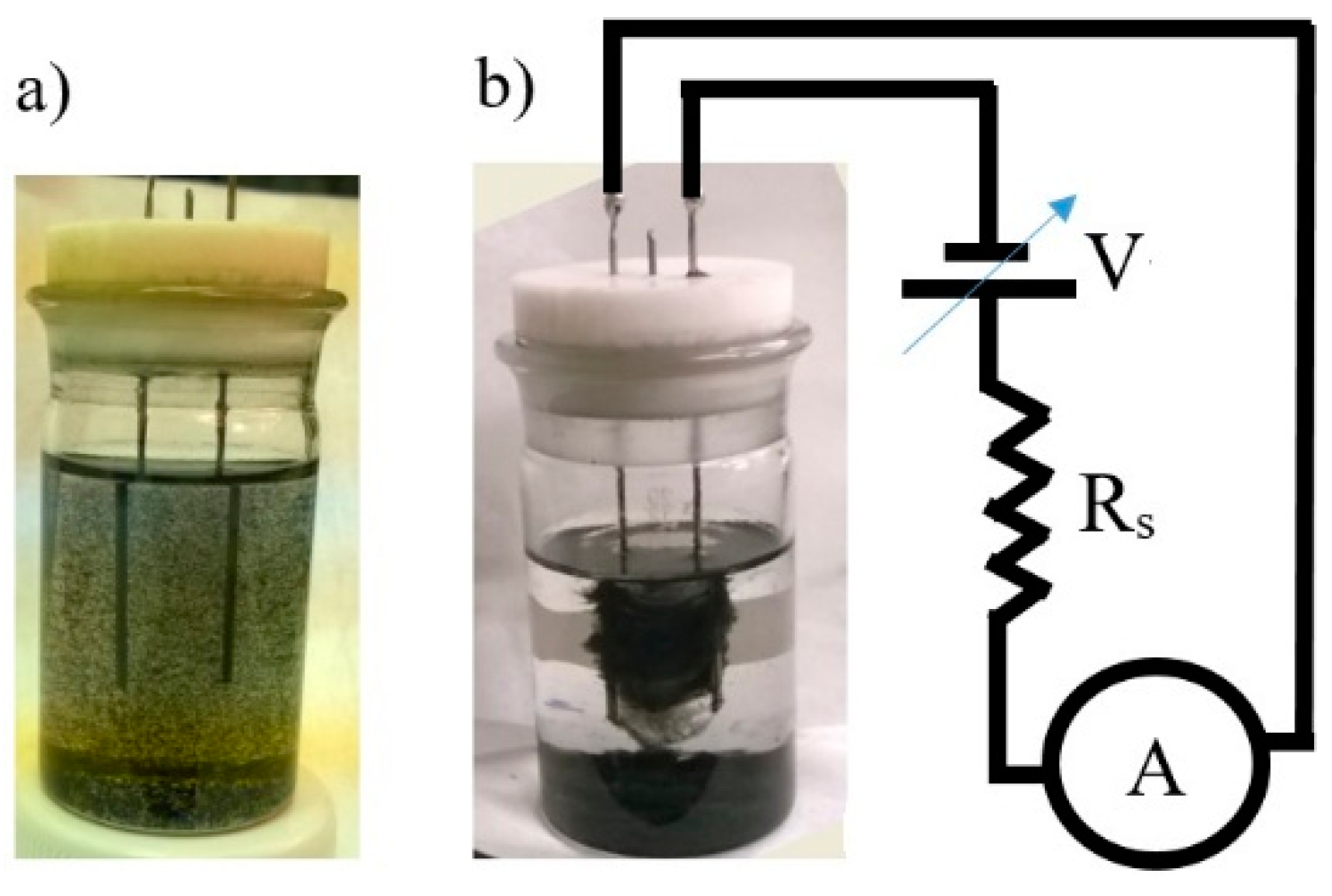
The system we study includes an adjustable voltage source (Keithley 6517B), V, a fixed resistor, R_s, connected in series with the voltage source and a self-assembly cell, which is connected in series with the resistor and the voltage source (Figure 2b). The ammeter, “A” (the same Keithley 6517B), which is also connected in series with the other elements, measures the current, I, in the circuit. The current is the same in all elements of the circuit. The self-assembly cell is a small glass vial with two needles inserted through its Teflon cap (Figure 2a,b). The design of the experimental setup is the same as in [40,41]. The self-assembly cell (the vial) is filled with a suspension of multiwall carbon nanotubes, dispersed in toluene. The toluene is chose because it has negligible electrical conductivity. Thus all the current measured in these experiments represents the current carried by the nanotubes, forming a cloud when voltage is applied. A homogeneous dispersion of nanotubes was prepared at the beginning of the measurements using a sonication bath. Typically the concentration of the nanotubes was in the range 0.1 to 0.4 mg/mL [42].

The physical mechanism of how the applied voltage and the corresponding electric field produce aligned conducting chains of nanotubes has been discussed in [41]. Briefly speaking, the mechanism is analogous to dielectrophoresis. Previously it has been applied, for example, to graphite nanoparticles but at a smaller scale [43,44]. It works as follows: the nanotubes are polarized be the electric field, like any conducting wire or molecule would, and therefore their positively charged ends are attracted to the negatively charged ends of their neighbors. Thus conducting chains of nanotubes form. Eventually the chains connect to the electrodes (the needles) and allow the current to flow in the circuit. The mechanism is analogous to the electrostatic trapping [43], developed for single metallic particles, but here it is applied to large ensembles of nanotubes, generalizing previous results [44]. The techniques of electrostatic trapping [43] and electrostatic self-assembly [44] apply to electrically conducting (i.e., metallic) particles, and carbon nanotubes can be good conductors of electricity [45]. Although here we use multiwall nanotubes, they should be even better conductors at room temperature due to their larger diameters. Note that the energy gap of the nanotube electronic spectrum is reduced as the nanotube radius is increased. Depending on the nanotube chirality, the energy gap can be zero in many cases.

The resistance, R, of the fluid (nanotubes+toluene), measured between the electrodes (Figure 2), is initially very large, ~10⁹ Ω (i.e., in the range of GΩ), because the nanotubes are disordered and toluene is a dielectric fluid. If a sufficiently high voltage is applied a self-assembly process begins, driven be the applied electric field [41]. In a certain range of the experimental parameters the nanotubes self-organize into a cloud surrounding the electrodes (Figure 2b). The cloud is electrically conducting, because each or almost each multiwall carbon nanotube is electrically conducting and the nanotubes connect to each other and form continuous chains within the cloud. If a sufficient evolution time is allowed, the resistance of the cloud attached to the electrodes tends to be of the order of the fixed series resistor, R ≈ R_s. The condition R ≈ R_s ensures that the power dissipated in the cloud is the maximum or near the maximum. One possible interpretation to such behavior is that the system adopts to the imposed conditions and self-organizes to maximize the entropy production. The technical reason of why the evolution halts or becomes very slow as R ≈ R_s is that at this level of self-organization the voltage on the fluid is already significantly reduced compared to the voltage applied by the source, simply because half of the applied potential drops on the series resistor. Any further ordering and any further reduction of the resistance of the nanotube cloud leads to further drop of the electric field in the fluid. Such reduction of the electric field prevents the evolution of the cloud from continuing further. This factor forces the evolution to become much slower at R < R_s compared to the initial stages where R >> R_s. Note that the voltage on the dissipative cloud is V₁ = V − IR_s = VR/(R + R_s). Obviously V₁ approaches zero if R approaches zero. As self-assembly proceeds and R drops, so does V₁. This should be a general property applicable to a wide range of systems with limited dissipation.

Since V₁ = RI is the voltage between the electrodes (Figure 2b), which is responsible for the ordering of the nanotubes, it is therefore natural to expect that at some point the ordering effect of the electric field will become comparable to the destructive forces of thermal fluctuations, vibrations, and gravity and thus the self-assembly process will become very slow. This is exactly what happens in experiments. As R becomes lower than R_s, the self-assembly progression becomes very slow and the resistance R remains near the level set by R_s, as long as the test continues. Such situation represents the impedance-matching condition, in which the power dissipated in the fluid is near its maximum. In some cases the resistance freezes exactly at the level defined by R = R_s, which represents the exact maximum. It is not understood why the systems sometimes satisfies MEPP approximately and in some situations with a high precision (i.e., within one percent or so).

Our system (Figure 2b) allows us to calculate and measure all essential quantities. In particular, the current in the circuit, according to Ohm’s law, is I = V/(R + R_s), because the self-assembly cell is connected in series with the resistor R_s. So the total Joule heating in the entire system is P_t = IV. We could not detect any difference in temperature inside the self-assembly cell compared to the environment [40], so we take it T = 293 K. Thus the total entropy production rate (i.e., the g-EPR) in the entire system is dS_t/dt = IV/T = V²/[T(R + R_s)]. The voltage V and the series resistor R_s are fixed during the evolution. The only adjustable part in the system is R, i.e., the resistance of the self-assembled cell, i.e., the resistance between the two needles. Note that R is defined by the number and the ordering of the carbon nanotubes connecting the needles. For example, if the nanotubes are parallel to each other the contact resistance between them should be much smaller compared to the case when the nanotubes are touching each other at random angles.

5. Experimental Results: “Successful” and “Unsuccessful” Evolution Scenarios

Evolution of partially ordered dissipative structures in our self-assembly cells can be broadly classified as “successful evolution” and “unsuccessful evolution”. The definitions of these notions are as follows. The successful evolution is such that it reaches the optimal current at which the rate of the entropy production inside the dissipative cloud is the maximum, i.e., dS/dt = (dS/dt)_max. This condition is classified as the DC-EPR maximum. This condition is practically possible and it requires the nanotubes to make a structure such that its resistance equals the series resistor in the circuit, i.e., R = R_s. The time needed to achieve the DC-EPR maximum is called the evolution time, t_e (below we present results indicating that t_e scales with the applied voltage as a power low). Once the maximum of the entropy production rate is achieved within the cloud, the entire system becomes stable, in the sense that the current can never drop below the level V/(2R_s), no matter how long we waited.

The unsuccessful evolution is a process in which the system is unable to organize to the extent that dS/dt = (dS/dt)_max, i.e., the system can never achieve the DC-EPR maximum. In this case the resistance between the needles remains larger than the series resistor in the circuit. In such case the development of the dissipative cloud cannot continue indefinitely. The structures formed under the effect of the applied field remain unstable if dS/dt < (dS/dt)_max. Sooner or later all or almost all nanotubes precipitate to the bottom of the self-assembly cell due to the effect of gravity. In this case they remain at the bottom indefinitely long. Thus dS/dt continues to drop and the chances that a strong dissipative cloud will form approach to zero. Thus unsuccessful evolution is not happening because we do not wait long enough time, but it is happening because nanotubes cannot form a stable cloud quickly enough and, as time goes by, they get removed from the self-assembly process completely, usually by gravity. Such two versions of the evolution have been observed in [41]. In the case of the so-called unsuccessful evolution the current was always observed to approach zero eventually, if we waited for a sufficiently long period of time.

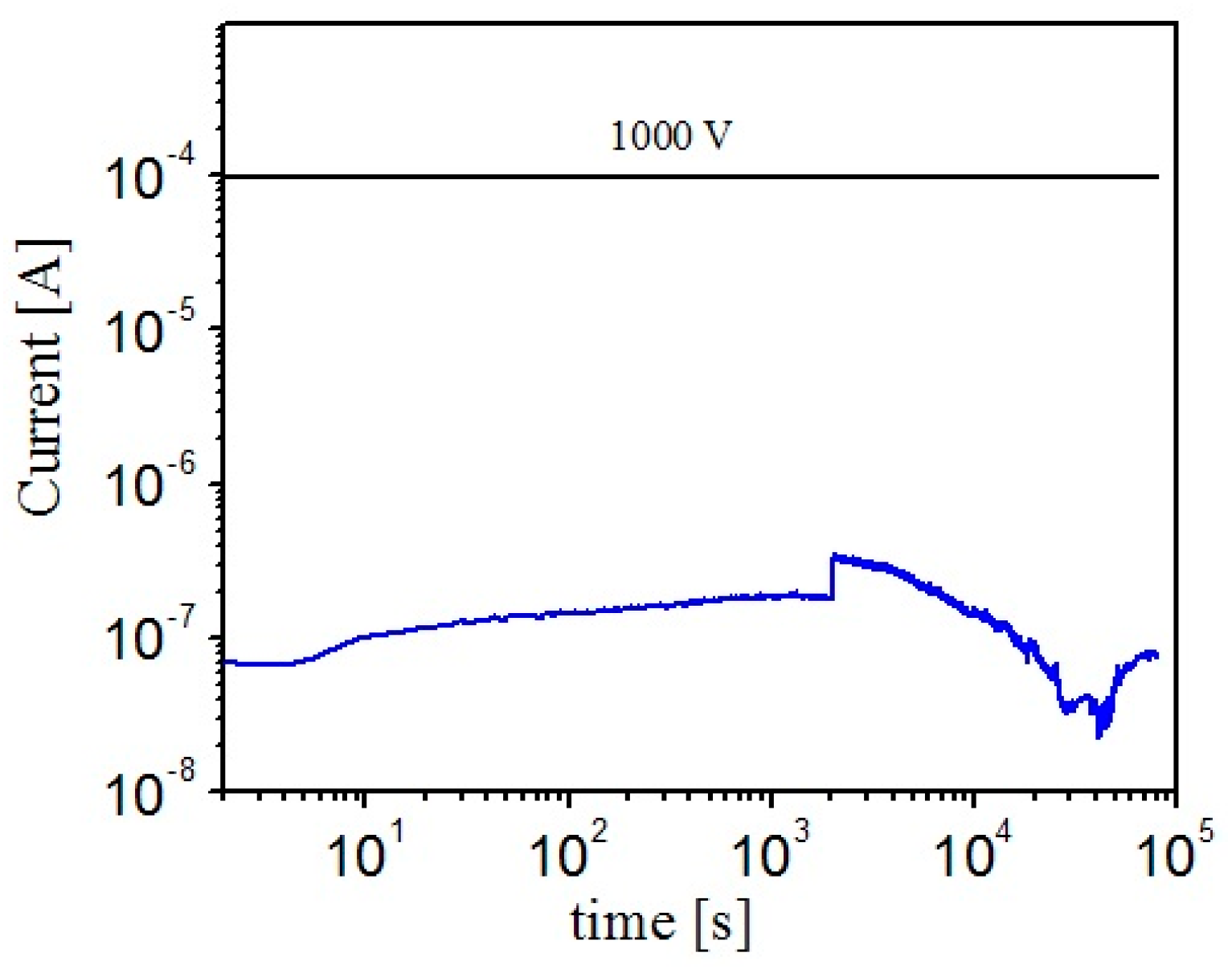
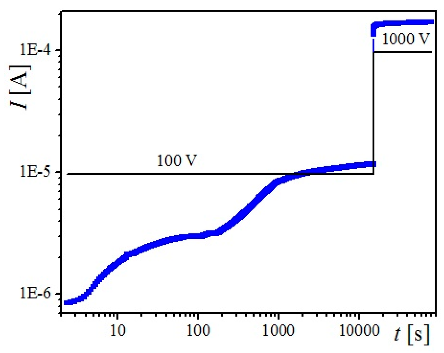
An example of a successful evolution is shown in Figure 3. In this case the system is allowed to evolve at 100 V bias first. A dissipative cloud of nanotubes forms rather quickly and achieves the maximum DC-EPR within 1796 s. After this we allowed this cloud to evolve for additional 13,484 s. During this additional time the current remained near the optimal value (more precisely slightly higher) and the entropy production was near the theoretically allowed maximum, dS/dt ≈ (dS/dt)_max. It was observed on other runs that even if the system is allowed for a longer evolution time, the dissipative cloud remained highly conducting and did not show any signs of deterioration, provided that the condition dS/dt ≥ (dS/dt)_max is achieved [41]. Note that S represents the entropy produced within the cloud, which should not be confused with the global or total entropy production rate in the entire circuit, S_t.

At t = 15,280 s a stability test was performed: The voltage was increased to 1000 V. After that the system remained in the state of the effective entropy generation, dS/dt ≈ (dS/dt)_max. This is a general observation: If the system has reached the maximum DC-EPR at a lower voltage, it remains stable and produces entropy at or near the maximum value if the voltage is strongly increase. Note that if the voltage would be set as high from the beginning of the experiment then the evolution would be unsuccessful, as will be shown below.

An example of an unsuccessful evolution is shown in Figure 4. In this experiment the voltage was too high for a stable pattern to naturally evolve. Thus dissipated power in the fluid with nanotubes was always low, less than 1% of the maximum possible power. Thus the entropy production was also less than 1% of the maximum possible. At the end of the evolution most of the nanotubes left the suspension and either precipitated on the bottom or were found stuck on the wall of the self-assembly cell.

Based on these and many similar experiments the behavior can be generalized as follows. As the voltage is applied the evolution of the dissipative cloud begins and entropy production goes up. If the optimal state of the DC-EPR maximum, i.e., R = R_s is achieved the resistance of the system either remains constant or slowly decreases in time. This means that the DC-EPR may be constant or slowly decrease, why g-EPR remains constant or slowly increases. The condition R < R_s represent a stability condition since one it is achieved the system never evolves to a less dissipative regime, R < R_s. One the other hand, if the system cannot achieve the regime R = R_s sufficiently quickly then both DC-EPT and g-EPR begin to decline, sooner or later, and eventually evolve to zero or very low values (unsuccessful evolution). If we use the language appropriate for biological living systems, then we can say that if the self-assembled dissipative cloud cannot reach its theoretical maximum of the entropy production rate then it “dies” eventually. But if the cloud can achieve the maximum DC-EPR then it “lives” forever.

6. The Impossibility to Achieve the Global Maximum of the Entropy Production Rate

The maximum g-EPR value, (dS_t/dt)_max = V²/(TR_s), would be achieved only if R = 0. Such situation of a perfect ordering is unattainable for the nanotube cloud, of course, because there is always some level of disorder in the nanotube dissipative cloud, so it is always true that R > 0. Thus the maximum of the global entropy production can never be achieved, i.e., (dS_t/dt) < (dS_t/dt)_max. Such rule should be a general property of any system in which the dissipation rate is limited, because the system has to achieve a perfect order (which is typically not possible) to produce heat at a maximum possible rate dissipation. Any real system can approach this level but cannot achieve it.

According to the simple analysis presented above our model system can be characterized as a system with limited dissipation: no matter how perfect the cloud of nanotubes is organized, it cannot dissipate more Joule heat than V²/R_s per second. Such limited dissipation condition is analogous to many real life situation. For example, in the example of an oil on hot plate (Figure 1), the energy provided to the hot plate is limited by the power of the heater. So if the oil can organize in a perfect array of convection cells, the heat flowing from the hot plate to the cold reservoir can approach the power of the hot plate, but can never exceed this limit. In reality the oil will always present some resistance to the heat flow. Thus, according to the principle suggested above, the entropy production would always be lower than the upper limit.

The general discussion of a system with limited dissipation leads to important general conclusions. It appears one cannot formulate MEPP as a statement that some certain level of g-EPR must be achieved. This is because the system can always drift or slowly evolve to approach the regime in which (dS_t/dt) = (dS_t/dt)_max, yet it is usually quite far from the regime in which g-EPR is maximum, which would require, in our context, a perfect organization in the dissipative structure so that it does not allow any potential to build up on itself.

So, if one suggests that a general law is the statement (dS_t/dt) = (dS_t/dt)_max then it is not true because no real dissipative system would have zero resistance and therefore in any practical situation we should have (dS_t/dt) < (dS_t/dt)_max. If we say that the true law of nature must be formulated as (dS_t/dt) = K(dS_t/dt)_max, where K is a constant such that K < 1, then it cannot be true either. The reason is that if the system achieves the regime (dS_t/dt) = K(dS_t/dt)_max then it can order a little bit more and achieve a state with even lower resistance and a higher value of dS_t/dt, i.e., the system can always progress to a state with (dS_t/dt) > K(dS_t/dt)_max. Thus the proposed modified equality will be violated at some point in time. If, on the other hand, the system can never reach the level of ordering characterized by some condition of the form (dS_t/dt) = K(dS_t/dt)_max then this condition would not be a true law also, because the system cannot achieve the regime characterized by this condition. Consequently a condition (dS_t/dt) = K(dS_t/dt)_max cannot describe a general law of nature either.

7. Two Possible Formulations of the Maximum Entropy Production Principle (MEPP)

In the systems where the source of the free energy and the self-organized system are distinguishable and separate, there are two ways to define the MEPP. The first formulation is to demand that the system is organized in such a way that the global entropy production (g-EPR) is maximized. This formulation cannot be always satisfied. For example, in our model system the global maximum is achieved only if R = 0, i.e., only if the cloud of nanotubes becomes superconducting. This is just not possible, because there is always contact resistance between the nanotubes and some level of disorder in the nanotubes. Thus, the formulation given above cannot be viewed as a general law, simply because it cannot be achieved, at least in our model system with limited dissipation. Perhaps it can be reformulated somehow. For example, one can say that the system approaches the global EPR maximum as time goes by but never achieves it.

A possible second formulation of the MEPP is to require that the entropy production within the dissipative cloud (DC-EPR) has to be maximized. It seems to be closely related to the local formulation proposed in [2,3]. The entropy produced in the cloud per unit time is dS/dt = V₁I/T. The maximum of this function is achieved if R = R_s. The corresponding maximum of the DC-EPR value is (dS/dt)_max = V²/(4TR_s). It was previously found [41] and confirmed here that the system can achieve this limit under a rather wide range of parameters. Thus the second definition of the MEPP appears to be more plausible. Practically, it is this condition which defines in many ways the behavior of the self-assembly cell. Thus it appears to be practically relevant for the description of evolution processes.

8. Our Proposed Formulation of the Maximum Entropy Production Principle (MEPP)

Our numerous experiments lead to the following conclusion: (1) dS/dt can achieve its theoretical maximum and plays an important role in defining the behavior of the system; (2) The g-EPR, dS_t/dt, can never achieve the maximum and does not even come close to the maximum in all experiments we have performed. Thus we always refer to the condition dS/dt = (dS/dt)_max as the regime of the maximum entropy production rate.

In our view this characteristics of systems with limited dissipation to always slowly approach but never being able to reach the g-EPR maximum makes the formulation of MEPP quite challenging: The correct principle cannot be stated as (dS_t/dt) = (dS_t/dt)_max and it cannot be stated as (dS_t/dt) = K(dS_t/dt)_max, where K is some constant less than one. This argument shows that the fourth law of thermodynamics, if it exists, cannot be formulated by saying that the global entropy production is the maximum, unless the maximum itself is understood very creatively, as some sort of a “moving target”. The only possible way to save the usual formulation of the MEPP is to admit that the maximum EPR is a time-dependent function. Our proposed idea is to use DC-EPR, rather than g-EPR, to formulate general rules of the system evolution.

In conclusion, if MEPP does hold as a general principle (as of now MEPP can be proven only in linear systems, but sometimes works in nonlinear systems also, for reasons which are not well understood), the principle will be formulated as dS/dt = (dS/dt)_max and not as dS_t/dt = (dS_t/dt)_max. This means that non-equilibrium thermodynamic systems are able and tend to maximize the entropy production in the self-assembly part of the system.

9. The “Training Effect”

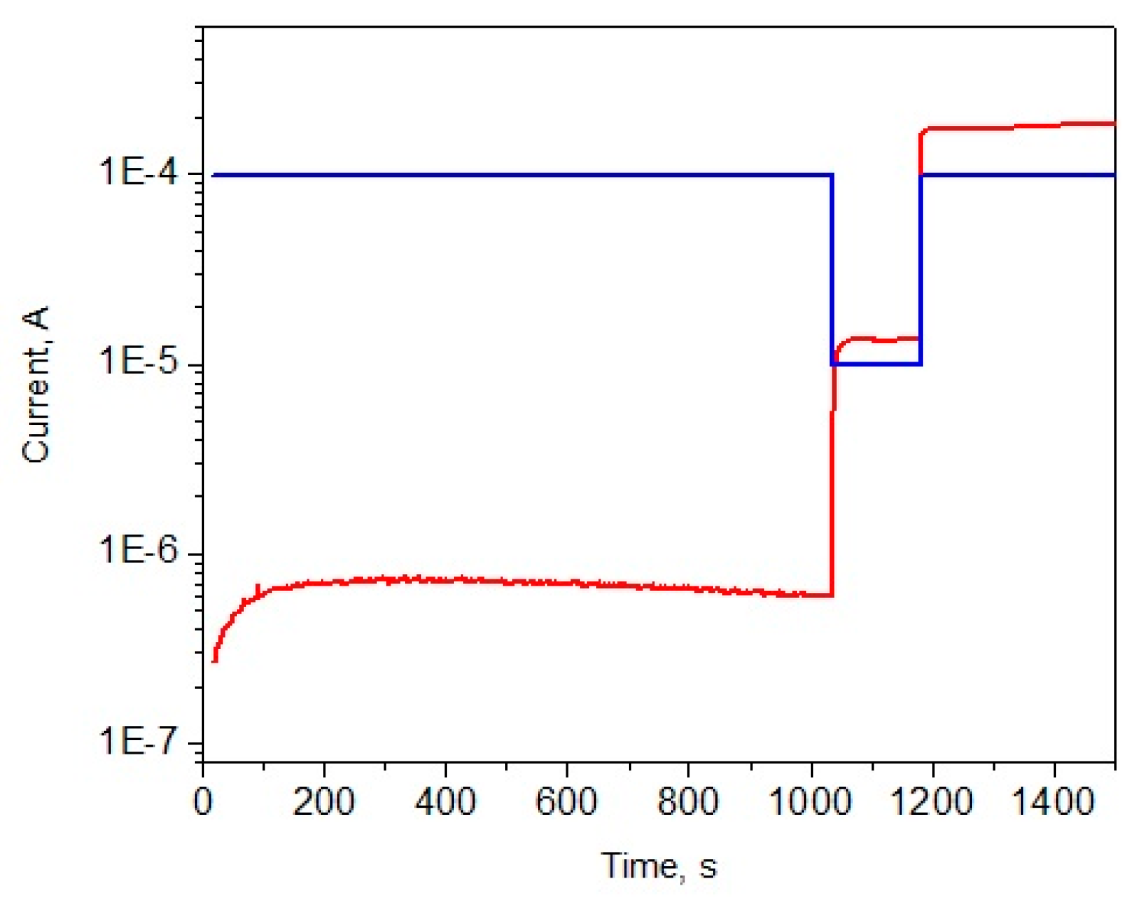
We have found external conditions (namely, high bias voltage) under which the maximum DC-EPR is possible in principle, but the system has to overcome some sort of an ordering barrier to get to the high DC-EPR regime. Under such conditions (namely, high bias voltage) the barrier is so significant that the system can never achieve the maximum of the entropy production rate (Figure 4). Yet, if a certain “help” is provided then the system can exist, practically indefinitely long, in the maximum DC-EPR regime without extenal help. Such inability to achieve the maximum DC-EPR regime, regardless the fact that such regime is clearly possible, was observed at high voltage bias, e.g., V = 1000 V for our typical parameters. In the example shown in Figure 5 the initial voltage bias was high, namely 1000 V. Such bias appeared to be too high for the system to form conducting chains [46]. Thus the DC-EPR stayed low as long as the 1000 V was maintained. Indeed, in the example typical graph of Figure 5 we observe that the current initially is very low, ≈ 0.7 μA, while the maximum rate dS/dt would be realized if the current would achieve 98 μA. In other words, the current has to be two orders of magnitude higher in order to produce the maximum possible amount of entropy per unit time, within the suspension. Then, at t = 1036 s the voltage was temporarily reduced to 100 V. This new voltage was within the range at which the suspended nanotubes were able to naturally self-organize into a conducting cloud and to achieve the optimal state in which the DC-EPR is maximized (or near the maximum possible), i.e., (dS/dt) ≈ (dS/dt)_max = V²/(4TR_s). The optimal current, I_opt = V/(2R_s), is shown by the blue horizontal lines in Figure 5. This is the current which, if achieved, ensures that the dissipative cloud of nanotubes generates the maximum possible amount of entropy per second. For the bias V = 100 V its value is I_opt = 9.8 μA. The nanotubes quickly, within just a few seconds, organize into an efficient cloud which achieves the maximum DC-EPR. The current achieved by the self-assembly cell is similar, namely 13.6 μA. This observation indicates that the evolution process frequently “overshoots” the exact value of the optimal current. Thus dS/dt appears slightly lower and dS_t/dt is slightly higher than it would be in the case I = I_opt.

The most important finding is that the dissipative cloud formed at 100 V remains stable even at much higher voltage. Indeed, at t = 1182 s the voltage was increased again to 1000 V. The dissipative cloud survived this ten-fold increase. The shape of the cloud changed only slightly. The cloud appears very similar to the one shown in Figure 2b. The current was again somewhat higher than the optimal current (Figure 5). Thus, at the high bias, the power dissipated within the self-assembled cloud was near it theoretical maximum. And, correspondingly, the entropy production was near its maximum too.

Figure 3 also shows an example of a training effect. There the system is allowed to evolve to the maximum DC-EPR regime at a low-range potential of V = 100 V. Then the voltage is switched to V = 1000 V. The system remains highly conducting and produces the entropy at a rate near the maximum possible. Yet, if the system would be evolving at V = 1000 V from the very beginning then it would not be able to approach the maximum DC-EPR regime, as is illustrated Figure 4.

The training effect outlined above confirms the existence of quasi-stable dissipative regimes in which the dissipation is much higher than in the more stable low-dissipation regime. The low DC-EPR regime is more stable because it represents the state in which the dissipative cloud does not form and the small current between the electrodes is carried out, probably, by electro-convection. The low-dissipation regime (Figure 4) progresses to the state in which all or most of the nanotube precipitate to the bottom of the convection cell. That is why its probability to switch to the highly-dissipative dissipative cloud state is negligibly low. On the other hand, we have observed, just once, that a low DC-EPR dynamic state suddenly switched to a high DC-EPR state, so the low DC-EPR regime is not absolutely stable. At the same time we have never seen a switch from a stable dissipative cloud, characterized by the stable regime condition, I > I_opt, to a low dissipation state. The question of stability of different dynamic dissipative states is not fully understood. Note that in this discussion the high-dissipation regime is such that the Joule heating power generated within the self-assembled nanotube cloud is of the order of the maximum possible value; the low-dissipation regime is such that the Joule heating power is much lower than the maximum possible value.

The existence of multiple metastable states is important since the existing models of the entropy production apparently neglects the possibility that the system can jump between different dynamic dissipative regimes, characterized by drastically different values of the entropy production rates. The existence of these regimes and the ability of the system to either high-dissipation or low-dissipation regimes, depending on chance and/or training, leads to a conclusion that the entropy production might not be at its maximum at all times. Thus, possibly, the MEPP should be understood probabilistically, as other principles of thermodynamics.

Possible physical reasons for the training effect exist. One possible explanation is that the newly formed chain attaches first to one of the electrodes, then it gets charged, very quickly, if the voltage is high. Consequently the chain gets repelled from the electrode and the self-assembly process get interrupted or pushed backward. When the voltage is reduced such Coulomb repulsion effect might not be sufficiently strong to interrupt the self-assembly process. Another alternative explanation is that the nanotubes become locally heated by the Joule dissipation when the resistance of the chain drops. Such local heating can interrupt the self-assembly due to an accelerated Brownian motion and enhanced thermal fluctuations. Again, if the voltage is reduced the effect of heating might not be critically significant. If many chains are formed, the collective effect of their parallel conductance is to reduce the voltage on the fluid (because more voltage drops on the series resistor if the resistance of the fluid is low). Thus when a large number of conducting chains is present then the system can withstand even a high voltage. Such collective effect has been discussed in [41] where experiments have been matched by a model.

10. Stability Critical Point R = R_s

The question of stability is of great importance [3]. In our experiments it was observed that if the current is equal or slightly higher than the optimal current the system is very stable. Even if the self-assembly cell is shaken to the extent that half of the dissipative cloud is destroyed, it is able to regenerate and to keep the current slightly above the optimal current, I_opt. Yet, if the damage done to the system is so strong that its current drops lower than I_opt then the system becomes unstable and immediately get dispersed by the high bias voltage. Such behavior is typically seen at a high bias, e.g., 1000 V, at which a low-voltage training session is, in general, needed to allow a highly dissipative cloud to form.

As was stated above the system remains unstable until the DC-EPR maximum is reached (thus we will illustrate the physical significance of the DC-EPR maximum). A useful example to illustrate this conclusion is the stability/instability against a voltage hike. For an illustration see Video S1 in the Supplementary Materials. In this experiment the system was allowed to evolve at V = 100 V for a sufficiently long time, so that a visible dissipative cloud was formed. Yet evolution time provided was not sufficient to reach the DC-EPR maximum, i.e., the resistance of the fluid remained high, R > R_s. Then the voltage was increased from 100 to 1000 V. This voltage hike was applied about 4 s after the beginning of the movie. Since the dissipative cloud was not able to reach the maximum of the CD-EPR during its preceding evolution, the cloud could not withstand this strong voltage increase. The movie shows how the dissipative cloud is quickly dispersed by the increased electric field. In this test the current was I/I_opt = 0.0038 before the voltage hike and the current became I/I_opt = 2.7 × 10⁻⁵ after the voltage was increased. The current dropped strongly due the fact that the applied voltage destroyed the dissipative cloud. Note that both of these current values represent the condition dS/dt << (dS/dt)_max.

Another example is shown in Video S2 in the Supplementary Materials. In this case the system was trained at 100 V and it was able to achieve the optimal entropy-generating regime I = I_opt and even moved up in current. At the moment of the test it was in the stable regime, i.e., R < R_s or, what is the same, I > I_opt. To demonstrate the stability of the dissipative cloud in this regime the voltage was increased by a factor of 10, about 18 second after the beginning of the movie. The dissipative cloud reshaped itself a little bit but remained stable and efficient to produce entropy. In this test the current was I = 1.05 I_opt before the voltage was increased and the current became I = 1.49 I_opt after the voltage hike. Both of these current values represent the condition dS/dt ~ (dS/dt)_max. Note that the cloud is the most dense between the needles; this is the region where most of the current is flowing.

These results (Video S1 and S2 and the damage test discussed above) illustrate that the point of the maximum DC-EPR, defined above as dS/dt = (dS/dt)_max, or, equivalently, as R = R_s, or as I = I_opt = V/2R_s, has a special significance as a stability-instability transition point. In other words, our experiments seem to suggest that the self-organizing system becomes stable when it realizes the maximum entropy production rate within itself. An analogous stabilization transition at R = R_s has been previously observed in a simple self-assembly model suggested in [41].

Based on these observations one can try to answer the question posed by Martyushev [2], namely the following: “However, the above question still remains: what forces the life to continuously develop and become more complex…?” A natural answer following from the analysis of the stability point is that the biological life evolution is governed by the dissipation limits set by the Sun. The life evolution should stop or become comparatively very slow only if the maximum possible dissipation (or entropy production) is achieved. This can only happen if a so-called “Dyson sphere” is constructed, which surrounds the entire Sun and captures all its radiation (and then the biological life forms, who created the sphere use this captured energy and eventually convert it into thermal radiation at a much lower temperature). Obviously this scenario represents a very distant future, if it ever happens at all. If the Dyson sphere is eventually constructed and the DC-EPR of the civilization reaches its maximum, then, if the analogy holds, the civilization and, probably, each of its elements, should become stable. Interestingly, this stability might imply, among other things, that some form of immortality will be achieved. Such scenario is suggested by the fact that, in our experiments, the dissipative cloud never “dies” after it has reached the DC-EPR maximum.

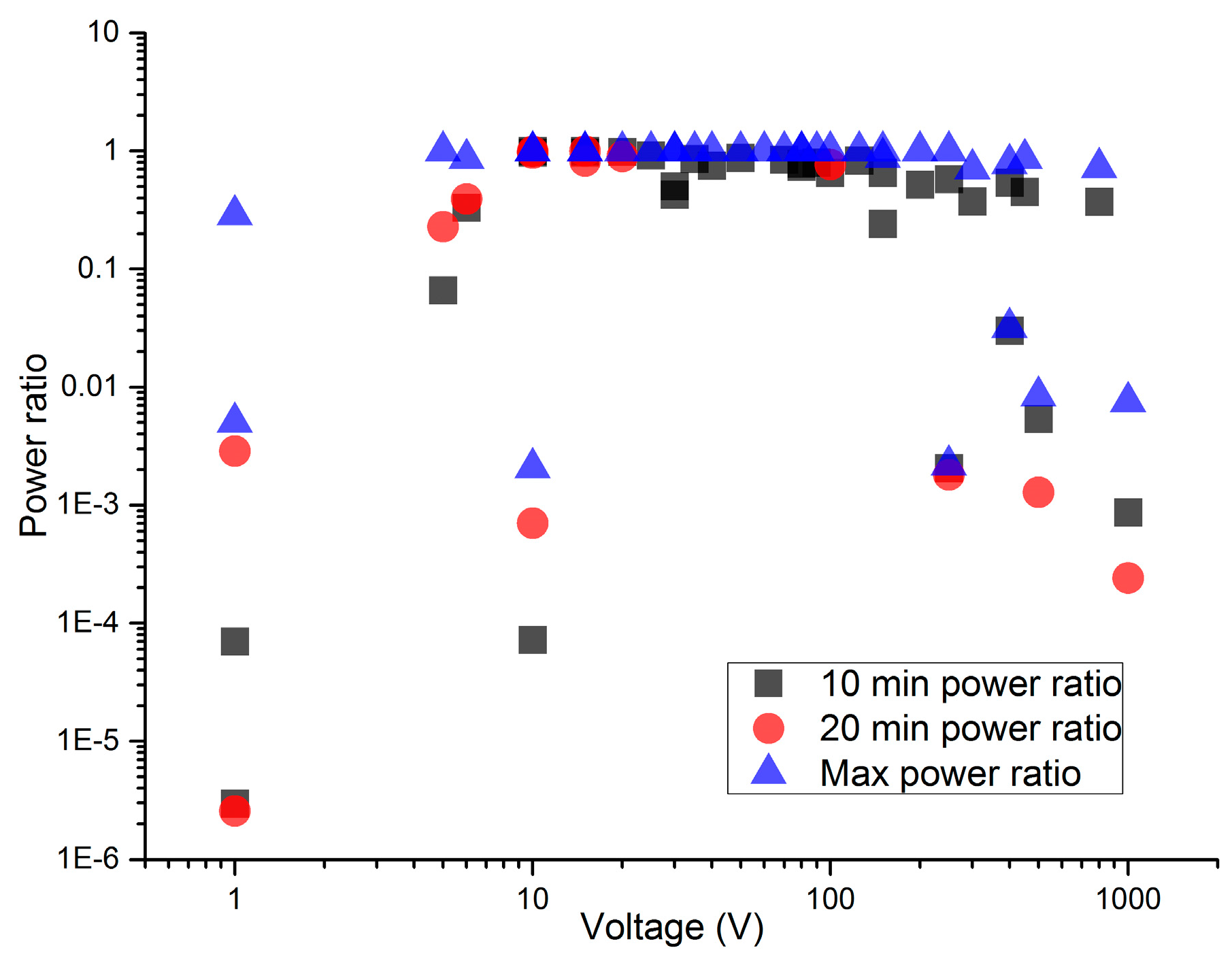
11. Range of Applicability

As the preceding paragraphs have shown, when an electric potential is applied to a suspension of nanotubes, the nanotubes will not always successfully self-assemble and reach the DC-EPR (the entropy production rate within the dissipative cloud) maximum. To determine the parameters where the nanotubes would successfully self-assemble, varying voltages were applied to a fixed concentration of multiwall nanotubes. The multiwall nanotubes were able to self-assemble and maximize their power production over more than an order of magnitude of applied voltage. Figure 6 shows the relationship between the level of organization of the system and the applied voltage.

In Figure 6, the different data points, measured after different evolution times, show the relation between self-assembly duration and increasing entropy production as a function of time. The unsuccessful trials between these voltages illustrate the randomizing effect of avalanches [41].

12. Power-Law Scaling of the Evolution Time with the Applied Voltage

Once the range of maximal entropy production for multiwall nanotubes was determined, an investigation was made into the relationship between the time required for a current to reach the maximal EPR in the self-assembly cell and the value of the applied voltage.

Experimental runs which did not reach the maximal rate of power production in the fluid were excluded from the analysis. In particular, an experiment was determined to have not reached the maximal power production rate if all or almost all the nanotubes had settled at the bottom of the container. Such runs are classified as unsuccessful evolution runs (see e.g., Figure 4). To determine if the nanotubes had settled out, the container was visually inspected to see if the toluene was transparent and no longer translucent or opaque from floating nanotubes and if the base of the container was black from a coating of nanotubes. Furthermore, the experiment was determined to have not reached maximal power if the power was two orders of magnitude below the maximum after 12 or more hours of testing. The two order of magnitude cutoff was chosen because no self-assembly events occurring after six hours have been ever observed to increase the power dissipation by over two orders of magnitude. Hence, the chance that a successful evolution test was ended too early can be considered practically zero. These cutoffs are justified because nanotubes in toluene are a suspension and not a solution, so once nanotubes settle on the bottom they cannot reenter the suspension, without sonication.

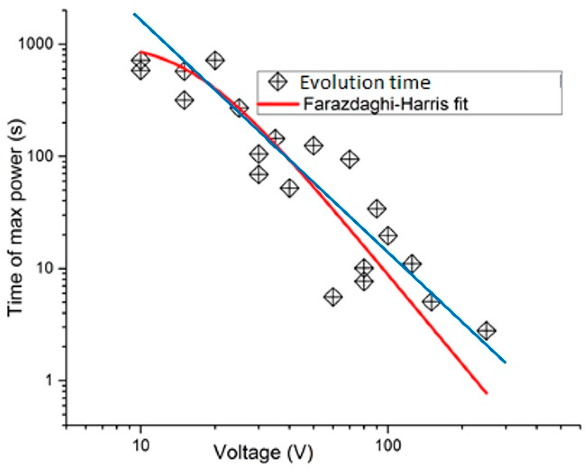
The results of multiple runs are summarized in Figure 7. There one can see that, approximately speaking, the evolution time scales as a power law with the applied voltage. In these logarithmic coordinates an exact power-law dependence would be a straight line. The data points appear to follow a linear dependence (blue line) approximately. Apart from the noise, there seems to be a systematic downward deviation from a straight line dependence at low bias voltage. This may be due to the effect mentioned above, namely the precipitation of carbon nanotubes at large time scales (note that if the nanotubes collect at the bottom before a dissipative cloud forms then the run will be classified as unsuccessful and no date point would be introduced to the plot).

The experimental data (Figure 7) can be best described mathematically using Farazdaghi–Harris fit, namely T_e = 1/(a + bV^c), where a and b are the fitting parameters and c is the best-fit exponent.

The results presented in this paragraphs seem to suggest that there is a power-law governing the evolution. Unfortunately the range of accessible voltages was limited to slightly more than one order of magnitude. To achieve a more substantial verification of this power-law dependence a different system, with a wider range of the thermodynamic potential should be found. Note that a power-law distribution of avalanches is a similar system has been reported in [41].

13. Conclusions

We have performed a series of experiments on a model system with limited dissipation. It is shown that the system cannot reach the maximum of the entropy production rate in the entire whole system, which includes the self-assembly cell and the voltage source and the series resistor. Yet it is found that the system can readily achieve the maximum rate of the entropy production within the self-assembled dissipative cloud, if the conditions are within the appropriate range of parameter and the system is allowed to evolve for a sufficiently long time. In some cases, to achieve this maximum the system needs a certain preliminary process, termed “training”, namely an initial stage of the evolution in which the system can evolve at a reduced potential and thus can develop a dissipative cloud. After the training stage the dissipative cloud can withstand a much higher potential, if and only if it was able to reach the maximum of the entropy production rate within the dissipative cloud (DC-EPR) during the training stage. Thus we suggest the maximum entropy production principle should be viewed as a stability threshold: The self-assembled non-equilibrium system becomes much more stable and, for example, can withstand a much higher bias if the maximum DC-EPR is reached.

14. Future Plans

(1) In order to further demonstrate the relevance of the entropy production rate we plan to study self-assembly processes at various temperatures. For example, two cells with suspended nanotubes can be connected in series. The cells will be maintained at different temperatures. Since the entropy production is proportional to the dissipated heat and inversely proportional to the temperature, one might expect that the cell with a lower temperatures should self-assemble more efficiently to allow a faster entropy production.

(2) Self-assembly with larger metallic spheres will be attempted. The goal is to make images and to analyze the fractal structure of the self-assembly pattern and to correlate this structure with the entropy production rate.

(3) We plan to study reproductive ability of the dissipative clouds. This question might be relevant in the situation when the voltage is high and the cloud cannot evolve on its own. It would be interesting to test if a new dissipative cloud develop after a small segment of a dissipative cloud formed in a separate environment is added to the fluid subjected to a high voltage.