1. Introduction
This paper concerns the efficiency of holographic heat engines, which were defined in [
1]. They are a natural concept in
extended gravitational thermodynamics, which, in making dynamical the cosmological constant (Λ) in a theory of gravity, supplies (here we are using geometrical units where
have been set to unity) a pressure variable
and its conjugate volume
V (see [
2,
3,
4,
5,
6,
7,
8,
9,
10,
11,
12,
13]).
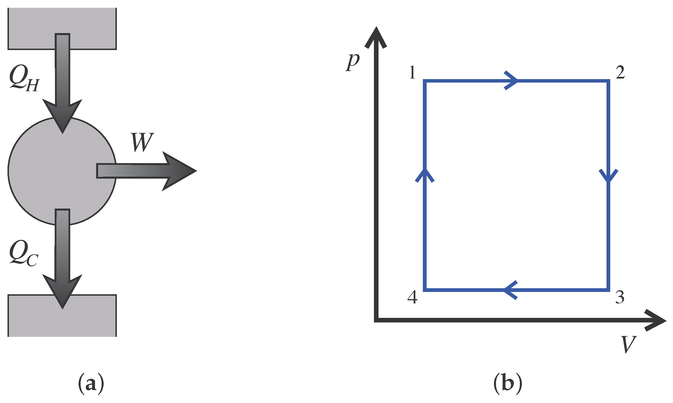
One may extract mechanical work via the
term in the First Law of Thermodynamics, and so it is possible to define a cycle in state space during which there is a net input heat
flow, a net output heat flow
, and a net output work
W such that
. See
Figure 1a. The efficiency is then
. Its value is determined by the equation of state of the system and the choice of cycle in state space. The gravitational solution (a black hole, in the cases studied here) supplies the equation of state: The temperature
T, entropy
S, and other quantities can be computed [
14,
15,
16,
17], and there are relations between them. There’s also a relation between the thermodynamic volume
V and the horizon radius of the black hole [
2]. The precise form of all these relations depends upon the type of black hole, and of course the parent theory of gravity under discussion. For example, [
18,
19] study the efficiency in the situation when the parent gravity theory has Gauss–Bonnet and Born–Infeld sectors.
In this extended thermodynamics context, we work with a negative cosmological constant (defining a positive pressure), for which such physics has an holographic duality [
20,
21,
22,
23,
24] to non–gravitational field theories in one dimension fewer, at large
N (where
N is the rank of a field theory gauge group, or an analogue thereof). This is why our heat engines in this context are called “holographic”. As pointed out in [
1], since changing Λ involves changing the
N of the dual theory, the heat engine cycle is a kind of tour on the
space of field theories rather than staying within one particular field theory (as pointed out in [
25] it also involves changing the size of the space the field theories live on). It is currently unclear as to the precise application of these heat engines in this context or any other, but as defined above they are certainly rich and well–defined enough in their own right to warrant an exploration of their physics.
For now, focus on the cycle given in
Figure 1b. In [
1], it is explained why such a choice is natural for static black holes, which we study here ([
18,
19,
26,
27,
28,
29] have since done further studies of such heat engines). The work performed is
, where the subscripts refer to the quantities evaluated at the corners labeled (1,2,3,4). In the absence of scalars, Isochors are also adiabats for static black holes (for the STU black holes, for example, it was shown in [
28] that the entropy and volume are independent functions, we thank an anonymous referee for suggesting this clarification), and so the heat flows take place entirely along the top and bottom, with the upper isobar giving the net inflow of heat and the lower isobar giving the exhaust:
where the specific heat at constant pressure
.
In the previous work on various black hole examples, the resulting efficiency
was evaluated in a high temperature limit, since in general, the relations between
S and
T are such that the
T–integral needed to evaluate
is difficult to perform exactly. [
18,
19] organize the computations of all needed quantities by working in terms of the horizon radius
, treating it as an independent parameter in terms of which all quantities can be most easily written. The high temperature expansions of all quantities were then developed by working out the high temperature expansion of
. It is worth noting here that a next logical step could be to recast the
T–integrals in Equation (
1) as
–integrals. Since
is (for some classes of black hole) a ratio of polynomials in
, depending upon the nature of the
Jacobian this might result in simpler expressions for the efficiency (this was also noted by Shao–Wen Wei, in a private communication). Indeed, as can be seen by evaluating a few examples, this is correct. In fact, there’s a much simpler way of looking at the whole picture that results in simple expression for the efficiency that makes it easy to see exactly why this works. We will explore this next.
2. A Simple Efficiency Formula
The key point is that when black holes are the focus, it is the enthalpy
H that takes center stage in the First Law of Thermodynamics, since it is identified with the mass
M of the black hole [
2]. So instead of writing the First Law in terms of the internal energy,
, one writes:
and since our heat flows are along isobars, for which
, we see immediately that our total heat flow
, regardless of which variable we care to write it in terms of, is simply the
enthalpy change, which is just the change in the black hole mass
M. Therefore, we have a remarkably simple way to write our efficiency formula entirely in terms of the black hole mass evaluated at the corners:
The mass
M is most naturally written as a function of
and
p. Depending upon which parameters of the cycle are prescribed (e.g., Scheme 1
or Scheme 2
in [
18,
19]), the equation of state can be readily used to evaluate the
and hence the mass values. In fact, if the parameters specified are all pressures and volumes (e.g.,
), the equation of state is not needed at all, (since the volume
V is a simple function of
) and the resulting exact efficiency formula is remarkably simple.
2.1. Examples
A nice class of examples is the static black hole of charge
q in
D dimensions that has mass formula:
where for
we are in Einstein–Maxwell gravity, and for non–zero
α we are in the Gauss–Bonnet generalization (see [
18,
30] for details and background; note that the Gauss–Bonnet extension is only non–trivial for
). The relationship between
and
p is given by:
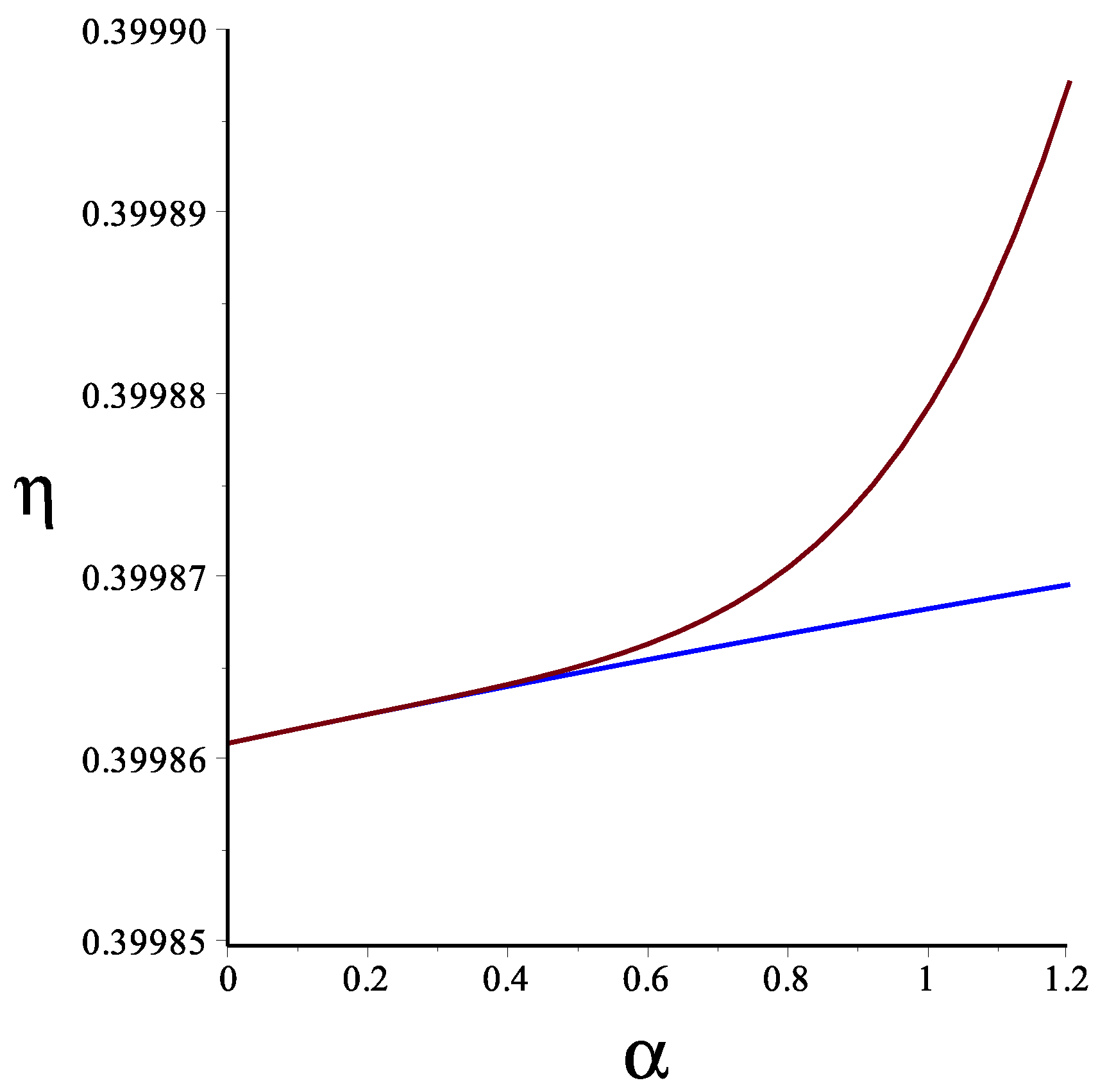
There is no need to work at high temperature, as our Formula (
3) is exact. In fact, it is pleasing to see how the high temperature expansion is corrected by it. In [
18], for a given chosen (large) temperature, the expansions begin to break down once
α gets too large. Using the formula to compute the exact efficiency is straightforward, and if (for example)
and
are specified parameters, one can invert Equation (
5) to compute the radii
and
, and compare to the result for the large
T procedures done in [
18]. Such an example is presented in
Figure 2. As
α increases, the deviation from accuracy (the upper curve is the large
T result) grows since the large
T expansion under-estimates the heat and over-estimates the work, as can be determined by a direct comparison of those quantities with the exact result.
3. The Efficiency for Arbitrary Cycles
Working out the efficiency of more general shapes of cycle is in principle difficult, since the specific heat along the cycle is in general quite complicated, even for static black holes. Computing the heat flows would be quite a challenge. A remarkable and immediate consequence of our result Equation (
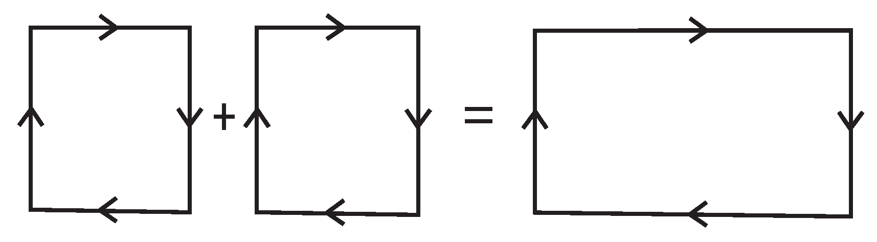
3) is that it can be used as the basis for an algorithm for computing the efficiency of a cycle of
arbitrary shape to any desired accuracy. The following describes how: Cycles are additive, in the sense indicated in
Figure 3, and any closed shape in the
plane can be approximated by tiling with a regular lattice of rectangles.
There will of course be parts where the tiling’s edge does not quite match the edge of the cycle’s contour. The amount of the failure can be reduced by simply shrinking the size of the unit cell. At any given desired degree of accuracy (cell size), the efficiency is computed simply as follows: Label all cells at the corners as was done for the prototype cycle in
Figure 1b. Only the cells at the edge contribute. They do so by either having their upper edge open (no adjoining cell), in which case we call it a hot cell, or by having their lower edge open, a cold cell. Summing all the hot cell mass differences (evaluated at the top edges) will give
and summing all the cold cell mass differences (evaluated at the bottom edges) will yield
, and the efficiency follows:
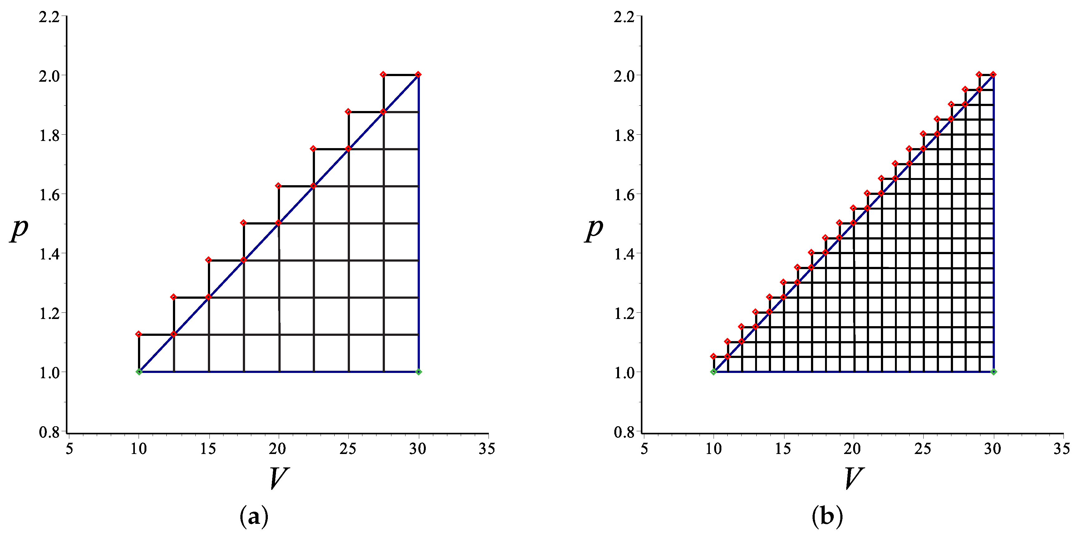
3.1. A Triangular Example
A triangular cycle was chosen to illustrate the algorithm in action. It has two edges parallel to the axes and one sloping edge in cycling from
values
to
to
and returning. One can choose to break it into a staircase–like rectangular lattice tiling that has
N rectangles (not to be confused with the
N of
Section 1) approximating the sloped edge, with better accuracy at larger
N, as in
Figure 4.
A simple procedure was coded for the computation of the required
and
p values for each cell, summing the contributions to
according to our Formula (
6). In this case
comes from the bottom edge as the overall mass difference along the base. Einstein–Maxwell black holes were used (
i.e., ), choosing the case
in Equation (
4) for the mass.
Figure 5 shows the rapid convergence toward the result as
N is increased.
4. Closing Remarks
A remarkably simple Expression (3) for the efficiency of a rectangular cycle for a class of static black holes was presented, simplifying earlier presented expressions and allowing it to be computed exactly. The whole formula is in terms of the black hole mass evaluated at each of the four corners of the cycle. Since the mass is often readily computable in a closed form expression, this is an extremely compact result.
Section 2.1 compared the results to the high temperature expansions obtained in earlier work.
While it might seem relevant only to a special class of cycle, the expression turns out to be quite powerful, being the seed of an algorithm for computing the efficiency of cycles of arbitrary shape using a well–defined geometrical procedure given in
Section 3. Such shapes would in general be hard to compute the efficiency for by, e.g., numerical integration methods along the path. The presented example (the triangle of
Section 3.1) shows how rapidly the algorithm converges to a result for the efficiency.
In fact, the procedure extends to wider classes of heat engine, whether a black hole is used as a working substance or not. The key object to be able to compute with is the basic unit cell needed to tile a cycle of arbitrary shape. More generally, the unit cell is actually a Brayton/Joule cycle, composed of two isobars and two adiabats. (In this paper it is a rectangle, since for static black holes (without scalars), adiabats are isochors). So all the heat flows are taken into account on the top and bottom edges. Since they are isobars, the heat flows can be written entirely in terms of the enthalpy. So for any system for which one can readily compute the enthalpy
H (and black holes turn out to be such a system since
H is simply the mass
M), and for which one knows the adiabatic curves, the same geometrical algorithm can be used to compute the efficiency of an arbitrary cycle in the manner described in
Section 3. It would be interesting to study some examples of this application.

