Maximizing Diversity in Biology and Beyond

Abstract

Entropy, under a variety of names, has long been used as a measure of diversity in ecology, as well as in genetics, economics and other fields. There is a spectrum of viewpoints on diversity, indexed by a real parameter q giving greater or lesser importance to rare species. Leinster and Cobbold (2012) proposed a one-parameter family of diversity measures taking into account both this variation and the varying similarities between species. Because of this latter feature, diversity is not maximized by the uniform distribution on species. So it is natural to ask: which distributions maximize diversity, and what is its maximum value? In principle, both answers depend on q, but our main theorem is that neither does. Thus, there is a single distribution that maximizes diversity from all viewpoints simultaneously, and any list of species has an unambiguous maximum diversity value. Furthermore, the maximizing distribution(s) can be computed in finite time, and any distribution maximizing diversity from some particular viewpoint $q>0$ actually maximizes diversity for all q. Although we phrase our results in ecological terms, they apply very widely, with applications in graph theory and metric geometry.

1. Introduction

For decades, ecologists have used entropy-like quantities as measures of biological diversity. The basic premise is that given a biological community or ecosystem containing n species in proportions $p_1,\dots ,p_n$, the entropy of the probability distribution $\left(p_i\right)$ indicates the extent to which the community is balanced or “diverse”. Shannon entropy itself is often used; so too are many variants, as we shall see. But almost all of them share the property that for a fixed number n of species, the entropy is maximized by the uniform distribution $p_i=1/n$.

However, there is a growing appreciation that this crude model of a biological community is too far from reality, in that it takes no notice of the varying similarities between species. For instance, we would intuitively judge a meadow to be more diverse if it consisted of ten dramatically different plant species than if it consisted of ten species of grass. This has led to the introduction of measures that do take into account inter-species similarities [1,2]. In mathematical terms, making this refinement essentially means extending the classical notion of entropy from probability distributions on a finite set to probability distributions on a finite metric space.

The maximum entropy problem now becomes more interesting. Consider, for instance, a pond community consisting of two very similar species of frog and one species of newt. We would not expect the maximum entropy (or diversity) to be achieved by the uniform distribution $(1/3,1/3,1/3)$, since the community would then be $2/3$ frog and only $1/3$ newt. We might expect the maximizing distribution to be closer to $(1/4,1/4,1/2)$; the exact answer should depend on the degrees of similarity of the species involved. We return to this scenario in Example 7.

For the sake of concreteness, this paper is written in terms of an ecological scenario: a community of organisms classified into species. However, nothing that we do is intrinsically ecological, or indeed connected to any specific branch of science. Our results apply equally to any collection of objects classified into types.

It is well understood that Shannon entropy is just one point (albeit a special one) on a continuous spectrum of entropies, indexed by a parameter $q\in [0,\infty ]$. This spectrum has been presented in at least two ways: as the Rényi entropies $H_q$ [3] and as the so-called Tsallis entropies $S_q$ (actually introduced as biodiversity measures by Patil and Taillie prior to Tsallis’s work in physics, and earlier still in information theory [4,5,6]):

$$H_q\left(\mathbf{p}\right)=\frac{1}{1-q}log\sum _{i=1}^n{p}_i^q,S_q\left(\mathbf{p}\right)=\frac{1}{q-1}\left(1-\sum _{i=1}^n{p}_i^q\right).$$

Both $H_q$ and $S_q$ converge to Shannon entropy as $q\to 1$. Moreover, $H_q$ and $S_q$ can be obtained from one another by an increasing invertible transformation, and in this sense are interchangeable.

When $H_q$ or $S_q$ is used as a diversity measure, q controls the weight attached to rare species, with $q=0$ giving as much importance to rare species as common ones and the limiting case $q=\infty$ reflecting only the prevalence of the most common species. Different values of q produce genuinely different judgements on which of two distributions is the more diverse. For instance, if over time a community loses some species but becomes more balanced, then the Rényi and Tsallis entropies decrease for $q=0$ but increase for $q=\infty$. Varying q therefore allows us to incorporate a spectrum of viewpoints on the meaning of the word “diversity”.

Here we use the diversity measures introduced by Leinster and Cobbold [1], which both (i) reflect this spectrum of viewpoints by including the variable parameter q, and (ii) take into account the varying similarities between species. We review these measures in Section 2, Section 3 and Section 4. In the extreme case where different species are assumed to have nothing whatsoever in common, they reduce to the exponentials of the Rényi entropies, and in other special cases they reduce to other diversity measures used by ecologists. In practical terms, the measures of [1] have been used to assess a variety of ecological systems, from communities of microbes [7,8] and crustacean zooplankton [9] to alpine plants [10] and arctic predators [11], as well as being applied in non-biological contexts such as computer network security [12].

Mathematically, the set-up is as follows. A biological community is modelled as a probability distribution $\mathbf{p}=(p_1,\dots ,p_n)$ (with $p_i$ representing the proportion of the community made up of species i) together with an $n\times n$ matrix $\mathbf{Z}$ (whose $(i,j)$-entry represents the similarity between species i and j). From this data, a formula gives a real number ${}^q{D}^{\mathbf{Z}}\left(\mathbf{p}\right)$ for each $q\in [0,\infty ]$, called the “diversity of order q” of the community. As for the Rényi entropies, different values of q make different judgements: for instance, it may be that for two distributions $\mathbf{p}$ and ${\mathbf{p}}^{\prime }$,

$${}^1{D}^{\mathbf{Z}}\left(\mathbf{p}\right)<{}^1{D}^{\mathbf{Z}}\left({\mathbf{p}}^{\prime }\right)\text{but}{}^2{D}^{\mathbf{Z}}\left(\mathbf{p}\right)>{}^2{D}^{\mathbf{Z}}\left({\mathbf{p}}^{\prime }\right).$$

Now consider the maximum diversity problem. Fix a list of species whose similarities to one another are known; that is, fix a matrix $\mathbf{Z}$ (subject to hypotheses to be discussed). The two basic questions are:

• Which distribution(s) $\mathbf{p}$ maximize the diversity ${}^q{D}^{\mathbf{Z}}\left(\mathbf{p}\right)$ of order q?
• What is the value of the maximum diversity ${sup}_{\mathbf{p}}{}^q{D}^{\mathbf{Z}}\left(\mathbf{p}\right)$?

This can be interpreted ecologically as follows: if we have a fixed list of species and complete control over their abundances within our community, how should we choose those abundances in order to maximize the diversity, and how large can we make that diversity?

In principle, both answers depend on q. After all, we have seen that if distributions are ranked by diversity then the ranking varies according to the value of q chosen. But our main theorem is that, in fact, both answers are independent of q:

Theorem 1 

(Main theorem). There exists a probability distribution on $\{1,\dots ,n\}$ that maximizes ${}^q{D}^{\mathbf{Z}}$ for all $q\in [0,\infty ]$. Moreover, the maximum diversity ${sup}_{\mathbf{p}}{}^q{D}^{\mathbf{Z}}\left(\mathbf{p}\right)$ is independent of $q\in [0,\infty ]$.

So, there is a “best of all possible worlds”: a distribution that maximizes diversity no matter what viewpoint one takes on the relative importance of rare and common species.

This theorem merely asserts the existence of a maximizing distribution. However, a second theorem describes how to compute all maximizing distributions, and the maximum diversity, in a finite number of steps (Theorem 2).

Better still, if by some means we have found a distribution $\mathbf{p}$ that maximizes the diversity of some order $q>0$, then a further result asserts that $\mathbf{p}$ maximizes diversity of all orders (Corollary 2). For instance, it is often easiest to find a maximizing distribution for diversity of order ∞ (as in Example 6 and Proposition 2), and it is then automatic that this distribution maximizes diversity of all orders.

Let us put these results into context. First, they belong to the huge body of work on maximum entropy problems. For example, the normal distribution has the maximum entropy among all probability distributions on $\mathbb{R}$ with a given mean and variance, a property which is intimately connected with its appearance in the central limit theorem. This alone would be enough motivation to seek maximum entropy distributions in other settings (such as the one at hand), quite apart from the importance of maximum entropy in thermodynamics, machine learning, macroecology, and so on.

Second, we will see that maximum diversity is very closely related to the emerging invariant known as magnitude. This is defined in the extremely wide generality of enriched category theory (Section 1 of [13]) and specializes in interesting ways in a variety of mathematical fields. For instance, it automatically produces a notion of the Euler characteristic of an (ordinary) category, closely related to the topological Euler characteristic [14]; in the context of metric spaces, magnitude encodes geometric information such as volume and dimension [15,16,17]; in graph theory, magnitude is a new invariant that turns out to be related to a graded homology theory for graphs [18,19]; and in algebra, magnitude produces an invariant of associative algebras that can be understood as a homological Euler characteristic [20].

This work is self-contained. To that end, we begin by explaining and defining the diversity measures in [1] (Section 2, Section 3 and Section 4). Then come the results: preparatory lemmas in Section 5, and the main results in Section 6 and Section 7. Examples are given in Section 8, Section 9 and Section 10, including results on special cases such as when the similarity matrix $\mathbf{Z}$ is either the adjacency matrix of a graph or positive definite. Perhaps counterintuitively, a distribution that maximizes diversity can eliminate some species entirely. This is addressed in Section 11, where we derive necessary and sufficient conditions on $\mathbf{Z}$ for maximization to preserve all species. Finally, we state some open questions (Section 12).

The main results of this paper previously appeared in a preprint of Leinster [21], but the proofs we present here are substantially simpler. Of the new results, Lemma 8 (the key to our results on preservation of species by maximizing distributions) borrows heavily from an argument of Fremlin and Talagrand [22].

Conventions

A vector $\mathbf{x}=(x_1,\dots ,x_n)\in {\mathbb{R}}^n$ is nonnegative if $x_i\ge 0$ for all i, and positive if $x_i>0$ for all i. The support of $\mathbf{x}\in {\mathbb{R}}^n$ is

$$supp\left(\mathbf{x}\right)=\left\{i\in \{1,\dots ,n\}:x_i\ne 0\right\},$$

and $\mathbf{x}$ has full support if $supp\left(\mathbf{x}\right)=\{1,\dots ,n\}$. A real symmetric $n\times n$ matrix $\mathbf{Z}$ is positive semidefinite if ${\mathbf{x}}^T\mathbf{Z}\mathbf{x}\ge 0$ for all $\mathbf{0}\ne \mathbf{x}\in {\mathbb{R}}^n$, and positive definite if this inequality is strict.

2. A Spectrum of Viewpoints on Diversity

Ecologists began to propose quantitative definitions of biological diversity in the mid-twentieth century [23,24], setting in motion more than fifty years of heated debate, dozens of further proposed diversity measures, hundreds of scholarly papers, at least one book devoted to the subject [25], and consequently, for some, despair (already expressed by 1971 in a famously-titled paper of Hurlbert [26]). Meanwhile, parallel discussions were taking place in disciplines such as genetics [27], economists were using the same formulas to measure wealth inequality and industrial concentration [28], and information theorists were developing the mathematical theory of such quantities under the name of entropy rather than diversity.

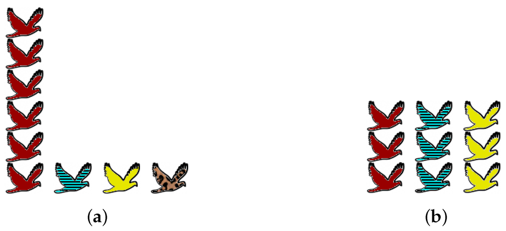
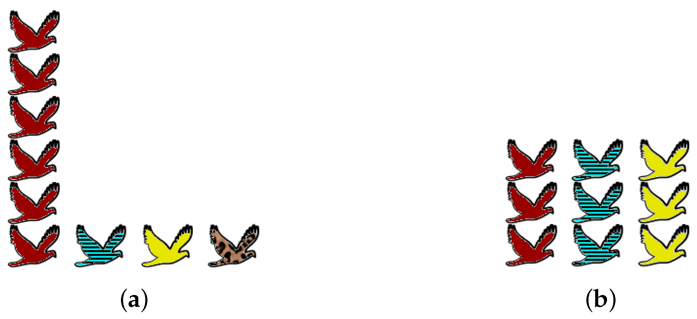
Obtaining accurate data about an ecosystem is beset with practical and statistical problems, but that is not the reason for the prolonged debate. Even assuming that complete information is available, there are genuine differences of opinion about what the word “diversity” should mean. We focus here on one particular axis of disagreement, illustrated by the examples in Figure 1.

Figure 1. Two bird communities. Heights of stacks indicate species abundances. In (a), there are four species, with the first dominant and the others relatively rare; in (b), the fourth species is absent but the community is otherwise evenly balanced.

One extreme viewpoint on diversity is that preservation of species is all that matters: “biodiversity” simply means the number of species present (as is common in the ecological literature as well as the media). Since no attention is paid to the abundances of the species present, rare species count for exactly as much as common species. From this viewpoint, community (a) of Figure 1 is more diverse than community (b), simply because it contains more species.

The opposite extreme is to ignore rare species altogether and consider only those that are most common. (This might be motivated by a focus on overall ecosystem function.) From this viewpoint, community (b) is more diverse than community (a), because it is better-balanced: (a) is dominated by a single common species, whereas (b) has three common species in equal proportions.

Between these two extremes, there is a spectrum of intermediate viewpoints, attaching more or less weight to rare species. Different scientists have found it appropriate to adopt different positions on this spectrum for different purposes, as the literature amply attests.

Rather than attempting to impose one particular viewpoint, we will consider all equally. Thus, we use a one-parameter family of diversity measures, with the “viewpoint parameter” $q\in [0,\infty ]$ controlling one’s position on the spectrum. Taking $q=0$ will give rare species as much importance as common species, while taking $q=\infty$ will give rare species no importance at all.

There is one important dimension missing from the discussion so far. We will consider not only the varying abundances of the species, but also the varying similarities between them. This is addressed in the next section.

3. Distributions on a Set with Similarities

In this section and the next, we give a brief introduction to the diversity measures of Leinster and Cobbold [1]. We have two tasks. We must build a mathematical model of the notion of “biological community” (this section). Then, we must define and explain the diversity measures themselves (next section).

In brief, a biological community will be modelled as a finite set (whose elements are the species) equipped with both a probability distribution (indicating the relative abundances of the species) and, for each pair of elements of the set, a similarity coefficient (reflecting the similarities between species).

Let us now consider each of these aspects in turn. First, we assume a community or system of individuals, partitioned into $n\ge 1$ species. The word “species” need not have its standard meaning: it can denote any unit thought meaningful, such as genus, serotype (in the case of viruses), or the class of organisms having a particular type of diet. It need not even be a biological grouping; for instance, in [29] the units are soil types. For concreteness, however, we write in terms of an ecological community divided into species. The division of a system into species or types may be somewhat artificial, but this is mitigated by the introduction of the similarity coefficients (as shown in [1], p. 482).

Second, each species has a relative abundance, the proportion of organisms in the community belonging to that species. Thus, listing the species in order as $1,\dots ,n$, the relative abundances determine a vector $\mathbf{p}=(p_1,\dots ,p_n)$. This is a probability distribution: $p_i\ge 0$ for each species i, and ${\sum }_{i=1}^n{p}_i=1$. Abundance can be measured in any way thought relevant, e.g., number of individuals, biomass, or (in the case of plants) ground coverage.

Critically, the word “diversity” refers only to the relative, not absolute, abundances. If half of a forest burns down, or if a patient loses $90\%$ of their gut bacteria, then it may be an ecological or medical disaster; but assuming that the system is well-mixed, the diversity does not change. In the language of physics, diversity is an intensive quantity (like density or temperature) rather than an extensive quantity (like mass or heat), meaning that it is independent of the system’s size.

The third and final aspect of the model is inter-species similarity. For each pair $(i,j)$ of species, we specify a real number $Z_{ij}$ representing the similarity between species i and j. This defines an $n\times n$ matrix $\mathbf{Z}={\left(Z_{ij}\right)}_{1\le i,j\le n}$. In [1], similarity is taken to be measured on a scale of 0 to 1, with 0 meaning total dissimilarity and 1 that the species are identical. Thus, it is assumed there that

$$0\le Z_{ij}\le 1\text{for}\text{all}i,j,Z_{ii}=1\text{for}\text{all}i.$$

(1)

In fact, our maximization theorems will only require the weaker hypotheses

$$Z_{ij}\ge 0\text{for}\text{all}i,j,Z_{ii}>0\text{for}\text{all}i$$

(2)

together with the requirement that $\mathbf{Z}$ is a symmetric matrix. (In the appendix to [1], matrices satisfying conditions (2) were called “relatedness matrices”.)

Just as the meanings of “species” and “abundance” are highly flexible, so too is the meaning of “similarity”:

Example 1. The simplest similarity matrix $\mathbf{Z}$ is the identity matrix $\mathbf{I}$. This is called the naive model in [1], since it embodies the assumption that distinct species have nothing in common. Crude though this assumption is, it is implicit in the diversity measures most popular in the ecological literature (Table 1 of [1] ).

Example 2. With the rapid fall in the cost of DNA sequencing, it is increasingly common to measure similarity genetically (in any of several ways). Thus, the coefficients $Z_{ij}$ may be chosen to represent percentage genetic similarities between species. This is an effective strategy even when the taxonomic classification is unclear or incomplete [1], as is often the case for microbial communities [7].

Example 3. Given a suitable phylogenetic tree, we may define the similarity between two present-day species as the proportion of evolutionary time before the point at which the species diverged.

Example 4. In the absence of more refined data, we can measure species similarity according to a taxonomic tree. For instance, we might define

$$Z_{ij}=\left\{\begin{array}{cc}1\hfill & \text{if}i=j,\hfill \\ 0.8\hfill & \text{if}\text{species}i\text{and}j\text{are}\text{different}\text{but}\text{of}\text{the}\text{same}\text{genus},\hfill \\ 0.5\hfill & \text{if}\text{species}i\text{and}j\text{are}\text{of}\text{different}\text{genera}\text{but}\text{the}\text{same}\text{family},\hfill \\ 0\hfill & \text{otherwise}.\hfill \end{array}\right.$$

Example 5. In purely mathematical terms, an important case is where the similarity matrix arises from a metric d on the set $\{1,\dots ,n\}$ via the formula $Z_{ij}=e^{-d(i,j)}$. Thus, the community is modelled as a probability distribution on a finite metric space. (The naive model corresponds to the metric defined by $d(i,j)=\infty$ for all $i\ne j$.) The diversity measures that we will shortly define can be understood as (the exponentials of) Rényi-like entropies for such distributions.

4. The Diversity Measures

Here we state the definition of the diversity measures of [1], which we will later seek to maximize. We then explain the reasons for this particular definition.

As in Section 3, we take a biological community modelled as a finite probability distribution $\mathbf{p}=(p_1,\dots ,p_n)$ together with an $n\times n$ matrix $\mathbf{Z}$ satisfying conditions (2). As explained in Section 2, we define not one diversity measure but a family of them, indexed by a parameter $q\in [0,\infty ]$ controlling the emphasis placed on rare species. The diversity of order q of the community is

$${}^q{D}^{\mathbf{Z}}\left(\mathbf{p}\right)={\left(\sum _{i\in supp\left(\mathbf{p}\right)}{p}_i{\left(\mathbf{Z}\mathbf{p}\right)}_i^{q-1}\right)}^{1/(1-q)}$$

(3)

($q\ne 1,\infty$). Here $supp\left(\mathbf{p}\right)$ is the support of $\mathbf{p}$ (Conventions, Section 1), $\mathbf{Z}\mathbf{p}$ is the column vector obtained by multiplying the matrix $\mathbf{Z}$ by the column vector $\mathbf{p}$, and ${\left(\mathbf{Z}\mathbf{p}\right)}_i$ is its i-th entry. Conditions (2) imply that ${\left(\mathbf{Z}\mathbf{p}\right)}_i>0$ whenever $i\in supp\left(\mathbf{p}\right)$, and so ${}^q{D}^{\mathbf{Z}}\left(\mathbf{p}\right)$ is well-defined.

Although this formula is invalid for $q=1$, it converges as $q\to 1$, and ${}^1{D}^{\mathbf{Z}}\left(\mathbf{p}\right)$ is defined to be the limit. The same is true for $q=\infty$. Explicitly,

$$\begin{array}{cc}\hfill {}^1{D}^{\mathbf{Z}}\left(\mathbf{p}\right)& =\prod _{i\in supp\left(\mathbf{p}\right)}{\left(\mathbf{Z}\mathbf{p}\right)}_i^{-p_i}=exp\left(-\sum _{i\in supp\left(\mathbf{p}\right)}{p}_{i}log{\left(\mathbf{Z}\mathbf{p}\right)}_i\right),\hfill \\ \hfill {}^{\infty }{D}^{\mathbf{Z}}\left(\mathbf{p}\right)& =1/\underset{i\in supp\left(\mathbf{p}\right)}{max}{\left(\mathbf{Z}\mathbf{p}\right)}_i.\hfill \end{array}$$

The applicability, context and meaning of Equation (3) are discussed at length in [1]. Here we briefly review the principal points.

First, the definition includes as special cases many existing quantities going by the name of diversity or entropy. For instance, in the naive model $\mathbf{Z}=\mathbf{I}$, the diversity ${}^q{D}^{\mathbf{I}}\left(\mathbf{p}\right)$ is the exponential of the Rényi entropy of order q, and is also known in ecology as the Hill number of order q. (References for this and the next two paragraphs are given in Table 1 of [1].)

Continuing in the naive model $\mathbf{Z}=\mathbf{I}$ and specializing further to particular values of q, we obtain other known quantities: ${}^0{D}^{\mathbf{I}}\left(\mathbf{p}\right)$ is species richness (the number of species present), ${}^1{D}^{\mathbf{I}}\left(\mathbf{p}\right)$ is the exponential of Shannon entropy, ${}^2{D}^{\mathbf{I}}\left(\mathbf{p}\right)$ is the Gini–Simpson index (the reciprocal of the probability that two randomly-chosen individuals are of the same species), and ${}^{\infty }{D}^{\mathbf{I}}\left(\mathbf{p}\right)=1/{max}_i{p}_i$ is the Berger–Parker index (a measure of the dominance of the most abundant species).

Now allowing a general $\mathbf{Z}$, the diversity of order 2 is $1/{\sum }_{i,j}{p}_i{Z}_{ij}{p}_j$. Thus, diversity of order 2 is the reciprocal of the expected similarity between a random pair of individuals. (The meaning given to “similarity” will determine the meaning of the diversity measure: taking the coefficients $Z_{ij}$ to be genetic similarities produces a genetic notion of diversity, and similarly phylogenetic, taxonomic, and so on.) Up to an increasing, invertible transformation, this is the well-studied quantity known as Rao’s quadratic entropy.

Given distributions $\mathbf{p}$ and ${\mathbf{p}}^{\prime }$ on the same list of species, different values of q may make different judgements on which of $\mathbf{p}$ and ${\mathbf{p}}^{\prime }$ is the more diverse. For instance, with $\mathbf{Z}=\mathbf{I}$ and the two distributions shown in Figure 1, taking $q=0$ makes community (a) more diverse and embodies the first “extreme viewpoint” described in Section 2, whereas $q=\infty$ makes (b) more diverse and embodies the opposite extreme.

It is therefore most informative if we calculate the diversity of all orders $q\in [0,\infty ]$. The graph of ${}^q{D}^{\mathbf{Z}}\left(\mathbf{p}\right)$ against q is called the diversity profile of $\mathbf{p}$. Two distributions $\mathbf{p}$ and ${\mathbf{p}}^{\prime }$ can be compared by plotting their diversity profiles on the same axes. If one curve is wholly above the other then the corresponding distribution is unambiguously more diverse. If they cross then the judgement as to which is the more diverse depends on how much importance is attached to rare species.

The formula for ${}^q{D}^{\mathbf{Z}}\left(\mathbf{p}\right)$ can be understood as follows.

First, for a given species i, the quantity ${\left(\mathbf{Z}\mathbf{p}\right)}_i={\sum }_j{Z}_{ij}{p}_j$ is the expected similarity between species i and an individual chosen at random. Differently put, ${\left(\mathbf{Z}\mathbf{p}\right)}_i$ measures the ordinariness of the i-th species within the community; in [1], it is called the “relative abundance of species similar to the i-th”. Hence, the mean ordinariness of an individual in the community is ${\sum }_i{p}_i{\left(\mathbf{Z}\mathbf{p}\right)}_i$. This measures the lack of diversity of the community, so its reciprocal is a measure of diversity. This is exactly ${}^2{D}^{\mathbf{Z}}\left(\mathbf{p}\right)$.

To explain the diversity of orders $q\ne 2$, we recall the classical notion of power mean. Let $\mathbf{p}=(p_1,\dots ,p_n)$ be a finite probability distribution and let $\mathbf{x}=(x_1,\dots ,x_n)\in {[0,\infty )}^n$, with $x_i>0$ whenever $p_i>0$. For real $t\ne 0$, the power mean of $\mathbf{x}$ of order t, weighted by $\mathbf{p}$, is

$$M_t(\mathbf{p},\mathbf{x})={\left(\sum _{i\in supp\left(\mathbf{p}\right)}{p}_i{x}_i^t\right)}^{1/t}$$

(Chapter II of [30]). This definition is extended to $t=0$ and $t=\pm \infty$ by taking limits in t, which gives

$$M_{-\infty }(\mathbf{p},\mathbf{x})=\underset{i\in supp\left(\mathbf{p}\right)}{min}{x}_i,M_0(\mathbf{p},\mathbf{x})=\prod _{i\in supp\left(\mathbf{p}\right)}{x}_i^{p_i},M_{\infty }(\mathbf{p},\mathbf{x})=\underset{i\in supp\left(\mathbf{p}\right)}{max}{x}_i.$$

Now, when we take the “mean ordinariness” in the previous paragraph, we can replace the ordinary arithmetic mean (the case $t=1$) by the power mean of order $t=q-1$. Again taking the reciprocal, we obtain exactly Equation (3). That is,

$${}^q{D}^{\mathbf{Z}}\left(\mathbf{p}\right)=1/M_{q-1}(\mathbf{p},\mathbf{Z}\mathbf{p})$$

(4)

for all $\mathbf{p}$, $\mathbf{Z}$, and $q\in [0,\infty ]$. So in all cases, diversity is the reciprocal mean ordinariness of an individual within the community, for varying interpretations of “mean”.

The diversity measures ${}^q{D}^{\mathbf{Z}}\left(\mathbf{p}\right)$ have many good properties, discussed in [1]. Crucially, they are effective numbers: that is,

$${}^q{D}^{\mathbf{I}}(1/n,\dots ,1/n)=n$$

for all q and n. This gives meaning to the quantities ${}^q{D}^{\mathbf{Z}}\left(\mathbf{p}\right)$: if ${}^q{D}^{\mathbf{Z}}\left(\mathbf{p}\right)=32.8$, say, then the community is nearly as diverse as a community of 33 completely dissimilar species in equal proportions. With the stronger assumptions (1) on $\mathbf{Z}$, the value of ${}^q{D}^{\mathbf{Z}}\left(\mathbf{p}\right)$ always lies between 1 and n.

Diversity profiles are decreasing: as less emphasis is given to rare species, perceived diversity drops. More precisely:

Proposition 1. 

Let $\mathbf{p}$ be a probability distribution on $\{1,\dots ,n\}$ and let $\mathbf{Z}$ be an $n\times n$ matrix satisfying conditions (2). If ${\left(\mathbf{Z}\mathbf{p}\right)}_i$ has the same value K for all $i\in supp\left(\mathbf{p}\right)$ then ${}^q{D}^{\mathbf{Z}}\left(\mathbf{p}\right)=1/K$ for all $q\in [0,\infty ]$. Otherwise, ${}^q{D}^{\mathbf{Z}}\left(\mathbf{p}\right)$ is strictly decreasing in $q\in [0,\infty ]$.

Proof. 

This is immediate from Equation (4) and a classical result on power means (Theorem 16 of [30]): $M_t(\mathbf{p},\mathbf{x})$ is increasing in t, strictly so unless $x_i$ has the same value K for all $i\in supp\left(\mathbf{p}\right)$, in which case it has constant value K. ☐

So, any diversity profile is either constant or strictly decreasing. The first part of the next lemma states that diversity profiles are also continuous:

Lemma 1. 

Fix an $n\times n$ matrix $\mathbf{Z}$ satisfying conditions (2). Then:

i.

${}^q{D}^{\mathbf{Z}}\left(\mathbf{p}\right)$ is continuous in $q\in [0,\infty ]$ for each distribution $\mathbf{p}$;

ii.

${}^q{D}^{\mathbf{Z}}\left(\mathbf{p}\right)$ is continuous in $\mathbf{p}$ for each $q\in (0,\infty )$.

Proof. 

See Propositions A1 and A2 of the appendix of [1]. ☐

Finally, the measures have the sensible property that if some species have zero abundance, then the diversity is the same as if they were not mentioned at all. To express this, we introduce some notation: given a subset $B\subseteq \{1,\dots ,n\}$, we denote by ${\mathbf{Z}}_B$ the submatrix ${\left(Z_{ij}\right)}_{i,j\in B}$ of $\mathbf{Z}$.

Lemma 2 

(Absent species). Let $\mathbf{Z}$ be an $n\times n$ matrix satisfying conditions (2). Let $B\subseteq \{1,\dots ,n\}$, and let $\mathbf{p}$ be a probability distribution on $\{1,\dots ,n\}$ such that $p_i=0$ for all $i\notin B$. Then, writing ${\mathbf{p}}^{\prime }$ for the restriction of $\mathbf{p}$ to B,

$${}^q{D}^{{\mathbf{Z}}_B}\left({\mathbf{p}}^{\prime }\right)={}^q{D}^{\mathbf{Z}}\left(\mathbf{p}\right)$$

for all $q\in [0,\infty ]$.

Proof. 

This is trivial, and is also an instance of a more general naturality property (Lemma A13 in the appendix of [1]). ☐

5. Preparatory Lemmas

For the rest of this work, fix an integer $n\ge 1$ and an $n\times n$ symmetric matrix $\mathbf{Z}$ of nonnegative reals whose diagonal entries are positive (that is, strictly greater than zero). Also write

$${\Delta }_n=\left\{(p_1,\dots ,p_n)\in {\mathbb{R}}^n:p_i\ge 0,p_1+\cdots +p_n=1\right\}$$

for the set of probability distributions on $\{1,\dots ,n\}$.

To prove the main theorem, we begin by making two apparent digressions.

Let $\mathbf{M}$ be any matrix. A weighting on $\mathbf{M}$ is a column vector $\mathbf{w}$ such that $\mathbf{M}\mathbf{w}$ is the column vector whose every entry is 1. It is trivial to check that if both $\mathbf{M}$ and its transpose have at least one weighting, then the quantity ${\sum }_i{w}_i$ is independent of the choice of weighting $\mathbf{w}$ on $\mathbf{M}$; this quantity is called the magnitude $\left|\mathbf{M}\right|$ of $\mathbf{M}$ (Section 1.1 of [13]).

When $\mathbf{M}$ is symmetric (the case of interest here), $\left|\mathbf{M}\right|$ is defined just as long as $\mathbf{M}$ has at least one weighting. When $\mathbf{M}$ is invertible, $\mathbf{M}$ has exactly one weighting and $\left|\mathbf{M}\right|$ is the sum of all the entries of ${\mathbf{M}}^{-1}$.

The second digression concerns the dichotomy expressed in Proposition 1: every diversity profile is either constant or strictly decreasing. We now ask: which distributions have constant diversity profile?

This question turns out to have a clean answer in terms of weightings and magnitude. To state it, we make some further definitions.

Definition 1. 

A probability distribution $\mathbf{p}$ on $\{1,\dots ,n\}$ is invariant if ${}^q{D}^{\mathbf{Z}}\left(\mathbf{p}\right)={}^{q^{\prime }}{D}^{\mathbf{Z}}\left(\mathbf{p}\right)$ for all $q,q^{\prime }\in [0,\infty ]$.

Let $B\subseteq \{1,\dots ,n\}$, and let $\mathbf{0}\ne \mathbf{w}\in {[0,\infty )}^B$ be a nonnegative vector. Then there is a probability distribution $\mathbf{p}\left(\mathbf{w}\right)$ on $\{1,\dots ,n\}$ defined by

$${\left(\mathbf{p}\left(\mathbf{w}\right)\right)}_i=\left\{\begin{array}{cc}{w}_i/\sum _{j\in B}{w}_j\hfill & \text{if}i\in B,\hfill \\ 0\hfill & \text{otherwise}.\hfill \end{array}\right.$$

In particular, let B be a nonempty subset of $\{1,\dots ,n\}$ and $\mathbf{w}$ a nonnegative weighting on ${\mathbf{Z}}_B={\left(Z_{ij}\right)}_{i,j\in B}$. Then $\mathbf{w}\ne \mathbf{0}$, so $\mathbf{p}\left(\mathbf{w}\right)$ is defined, and $\mathbf{p}{\left(\mathbf{w}\right)}_i=w_i/\left|{\mathbf{Z}}_B\right|$ for all $i\in B$.

Lemma 3. 

The following are equivalent for $\mathbf{p}\in {\Delta }_n$:

i.

$\mathbf{p}$ is invariant;

ii.

${\left(\mathbf{Z}\mathbf{p}\right)}_i={\left(\mathbf{Z}\mathbf{p}\right)}_j$ for all $i,j\in supp\left(\mathbf{p}\right)$;

iii.

$\mathbf{p}=\mathbf{p}\left(\mathbf{w}\right)$ for some nonnegative weighting $\mathbf{w}$ on ${\mathbf{Z}}_B$ and some nonempty subset $B\subseteq \{1,\dots ,n\}$.

Moreover, in the situation of (iii), ${}^q{D}^{\mathbf{Z}}\left(\mathbf{p}\right)=\left|{\mathbf{Z}}_B\right|$ for all $q\in [0,\infty ]$.

Proof. 

(i) $\underset{\hspace{1em}\hspace{1em}}{\iff }$ (ii) is immediate from Proposition 1.

For (ii) $\underset{\hspace{1em}\hspace{1em}}{\Rightarrow }$ (iii), assume (ii). Put $B=supp\left(\mathbf{p}\right)$ and write $K={\left(\mathbf{Z}\mathbf{p}\right)}_i$ for any $i\in B$. Then $K>0$, so we may define $\mathbf{w}\in {\mathbb{R}}^B$ by $w_i=p_i/K$ ($i\in B$). Evidently $\mathbf{p}=\mathbf{p}\left(\mathbf{w}\right)$ and $\mathbf{w}$ is nonnegative. Furthermore, $\mathbf{w}$ is a weighting on ${\mathbf{Z}}_B$, since whenever $i\in B$,

$${\left({\mathbf{Z}}_B\mathbf{w}\right)}_i=\sum _{j\in B}{Z}_{ij}{p}_j/K=\sum _{j=1}^n{Z}_{ij}{p}_j/K=1.$$

Finally, for (iii) $\underset{\hspace{1em}\hspace{1em}}{\Rightarrow }$ (ii) and “moreover”, take B and $\mathbf{w}$ as in (iii). Then $supp\left(\mathbf{p}\right(\mathbf{w}\left)\right)\subseteq B$, so for all $i\in supp\left(\mathbf{p}\right(\mathbf{w}\left)\right)$,

$${\left(\mathbf{Z}·\mathbf{p}\left(\mathbf{w}\right)\right)}_i={\left({\mathbf{Z}}_B\mathbf{w}/\left|{\mathbf{Z}}_B\right|\right)}_i=1/\left|{\mathbf{Z}}_B\right|.$$

Hence ${}^q{D}^{\mathbf{Z}}\left(\mathbf{p}\left(\mathbf{w}\right)\right)=\left|{\mathbf{Z}}_B\right|$ for all $q\in [0,\infty ]$ by Proposition 1. ☐

We now prove a result that is much weaker than the main theorem, but will act as a stepping stone in the proof.

Lemma 4. 

For each $q\in (0,1)$, there exists an invariant distribution that maximizes ${}^q{D}^{\mathbf{Z}}$.

Proof. 

Let $q\in (0,1)$. Then ${}^q{D}^{\mathbf{Z}}$ is continuous on the compact space ${\Delta }_n$ (Lemma 1(ii)), so attains a maximum at some point $\mathbf{p}$. Take $j,k\in supp\left(\mathbf{p}\right)$ such that ${\left(\mathbf{Z}\mathbf{p}\right)}_j$ is least and ${\left(\mathbf{Z}\mathbf{p}\right)}_k$ is greatest. By Lemma 3, it is enough to prove that ${\left(\mathbf{Z}\mathbf{p}\right)}_j={\left(\mathbf{Z}\mathbf{p}\right)}_k$.

Define ${\delta }_j\in {\Delta }_n$ by taking ${\left({\delta }_j\right)}_i$ to be the Kronecker delta ${\delta }_{ji}$, and ${\delta }_k$ similarly. Then $\mathbf{p}+t({\delta }_j-{\delta }_k)\in {\Delta }_n$ for all real t sufficiently close to 0, and

$$\begin{array}{cc}\hfill 0& =\frac{d}{dt}\left({}^q{D}^{\mathbf{Z}}{\left(\mathbf{p}+t({\delta }_j-{\delta }_k)\right)}^{1-q}\right){|}_{t=0}\hfill \end{array}$$

(5)

$$\begin{array}{cc}& =(q-1)\left(\sum _{i\in supp\left(\mathbf{p}\right)}{Z}_{ij}{p}_i{\left(\mathbf{Z}\mathbf{p}\right)}_i^{q-2}-\sum _{i\in supp\left(\mathbf{p}\right)}{Z}_{ik}{p}_i{\left(\mathbf{Z}\mathbf{p}\right)}_i^{q-2}\right)+{\left(\mathbf{Z}\mathbf{p}\right)}_j^{q-1}-{\left(\mathbf{Z}\mathbf{p}\right)}_k^{q-1}\hfill \end{array}$$

(6)

$$\begin{array}{cc}& \ge (q-1)\left(\sum _{i=1}^n{Z}_{ij}{p}_i{\left(\mathbf{Z}\mathbf{p}\right)}_j^{q-2}-\sum _{i=1}^n{Z}_{ik}{p}_i{\left(\mathbf{Z}\mathbf{p}\right)}_k^{q-2}\right)+{\left(\mathbf{Z}\mathbf{p}\right)}_j^{q-1}-{\left(\mathbf{Z}\mathbf{p}\right)}_k^{q-1}\hfill \end{array}$$

(7)

$$\begin{array}{cc}& =q\left({\left(\mathbf{Z}\mathbf{p}\right)}_j^{q-1}-{\left(\mathbf{Z}\mathbf{p}\right)}_k^{q-1}\right)\hfill \end{array}$$

(8)

$$\begin{array}{cc}& \ge 0,\hfill \end{array}$$

(9)

where Equation (5) holds because $\mathbf{p}$ is a supremum, Equation (6) is a routine computation, inequalities (7) and (9) follow from the defining properties of j and k, and Equation (8) uses the symmetry of $\mathbf{Z}$. Equality therefore holds throughout, and in particular in (9). Hence ${\left(\mathbf{Z}\mathbf{p}\right)}_j={\left(\mathbf{Z}\mathbf{p}\right)}_k$, as required. ☐

An alternative proof uses Lagrange multipliers, but is complicated by the possibility that ${}^q{D}^{\mathbf{Z}}$ attains its maximum on the boundary of ${\Delta }_n$.

The result we have just proved only concerns the maximization of ${}^q{D}^{\mathbf{Z}}$ for specific values of q, but the following lemma will allow us to deduce results about maximization for all q simultaneously.

Definition 2. 

A probability distribution on $\{1,\dots ,n\}$ is maximizing if it maximizes ${}^q{D}^{\mathbf{Z}}$ for all $q\in [0,\infty ]$.

Lemma 5. 

For $0\le q^{\prime }\le q\le \infty$, any invariant distribution that maximizes ${}^{q^{\prime }}{D}^{\mathbf{Z}}$ also maximizes ${}^q{D}^{\mathbf{Z}}$. In particular, any invariant distribution that maximizes ${}^0{D}^{\mathbf{Z}}$ is maximizing.

Proof. Let $0\le q^{\prime }\le q\le \infty$ and let $\mathbf{p}$ be an invariant distribution that maximizes ${}^{q^{\prime }}{D}^{\mathbf{Z}}$. Then for all $\mathbf{r}\in {\Delta }_n$,

$${}^q{D}^{\mathbf{Z}}\left(\mathbf{r}\right)\le {}^{q^{\prime }}{D}^{\mathbf{Z}}\left(\mathbf{r}\right)\le {}^{q^{\prime }}{D}^{\mathbf{Z}}\left(\mathbf{p}\right)={}^q{D}^{\mathbf{Z}}\left(\mathbf{p}\right),$$

since diversity profiles are decreasing (Proposition 1). ☐

6. The Main Theorem

For convenience, we restate the main theorem:

Theorem 1 

(Main theorem). There exists a probability distribution on $\{1,\dots ,n\}$ that maximizes ${}^q{D}^{\mathbf{Z}}$ for all $q\in [0,\infty ]$. Moreover, the maximum diversity ${sup}_{\mathbf{p}\in {\Delta }_n}{}^q{D}^{\mathbf{Z}}\left(\mathbf{p}\right)$ is independent of $q\in [0,\infty ]$.

Proof. 

An equivalent statement is that there exists an invariant maximizing distribution. To prove this, choose a decreasing sequence ${\left(q_{\lambda }\right)}_{\lambda =1}^{\infty }$ in $(0,1)$ converging to 0. By Lemma 4, we can choose for each $\lambda \ge 1$ an invariant distribution ${\mathbf{p}}^{\lambda }$ that maximizes ${}^{q_{\lambda }}{D}^{\mathbf{Z}}$. Since ${\Delta }_n$ is compact, we may assume (by passing to a subsequence if necessary) that the sequence $\left({\mathbf{p}}^{\lambda }\right)$ converges to some point $\mathbf{p}\in {\Delta }_n$. We will show that $\mathbf{p}$ is invariant and maximizing.

We show that $\mathbf{p}$ is invariant using Lemma 3. Let $i,j\in supp\left(\mathbf{p}\right)$. Then $i,j\in supp\left({\mathbf{p}}^{\lambda }\right)$ for all $\lambda \gg 0$, so ${\left(\mathbf{Z}{\mathbf{p}}^{\lambda }\right)}_i={\left(\mathbf{Z}{\mathbf{p}}^{\lambda }\right)}_j$ for all $\lambda \gg 0$, and letting $\lambda \to \infty$ gives ${\left(\mathbf{Z}\mathbf{p}\right)}_i={\left(\mathbf{Z}\mathbf{p}\right)}_j$.

To show that $\mathbf{p}$ is maximizing, first note that ${\mathbf{p}}^{{\lambda }^{\prime }}$ maximizes ${}^{q_{\lambda }}{D}^{\mathbf{Z}}$ whenever ${\lambda }^{\prime }\ge \lambda \ge 1$ (by Lemma 5). Fixing λ and letting ${\lambda }^{\prime }\to \infty$, this implies that $\mathbf{p}$ maximizes ${}^{q_{\lambda }}{D}^{\mathbf{Z}}$, since ${}^{q_{\lambda }}{D}^{\mathbf{Z}}$ is continuous (Lemma 1(ii)).

Thus, $\mathbf{p}$ maximizes ${}^{q_{\lambda }}{D}^{\mathbf{Z}}$ for all λ. But $q_{\lambda }\to 0$ as $\lambda \to \infty$, and diversity is continuous in its order (Lemma 1(i)), so $\mathbf{p}$ maximizes ${}^0{D}^{\mathbf{Z}}$. Since $\mathbf{p}$ is invariant, Lemma 5 implies that $\mathbf{p}$ is maximizing. ☐

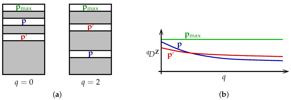
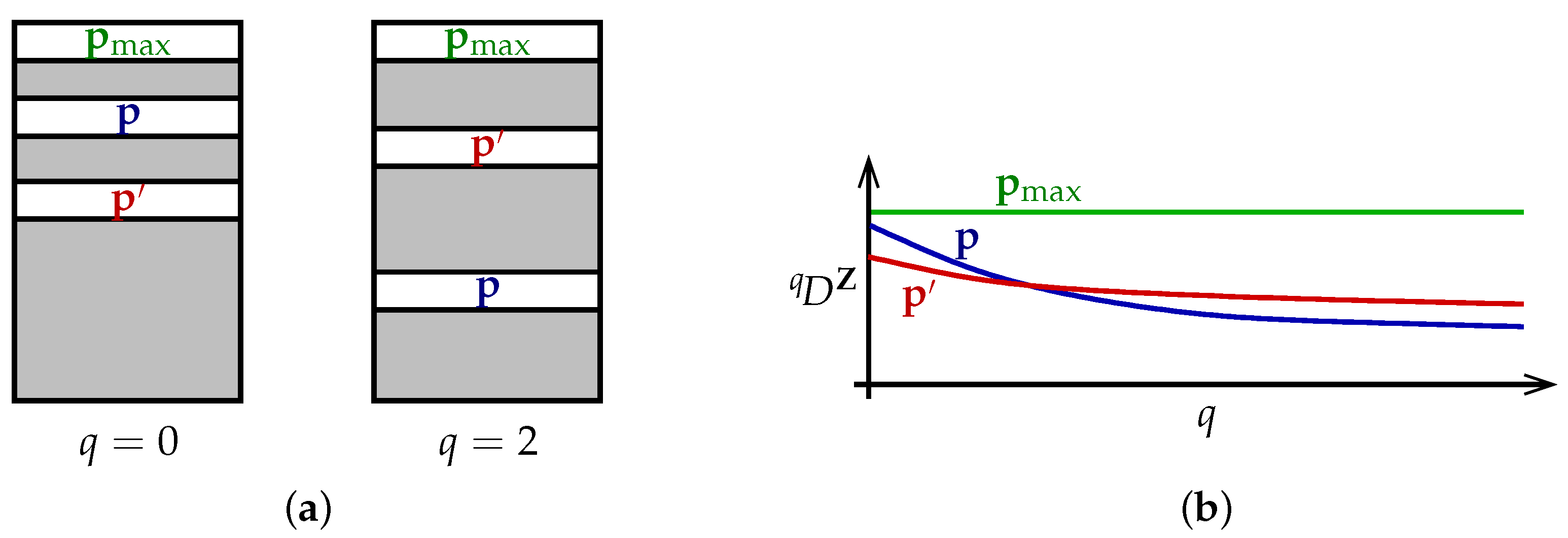
The theorem can be understood as follows (Figure 2a). Each particular value of the viewpoint parameter q ranks the set of all distributions $\mathbf{p}$ in order of diversity, with $\mathbf{p}$ placed above ${\mathbf{p}}^{\prime }$ when ${}^q{D}^{\mathbf{Z}}\left(\mathbf{p}\right)>{}^q{D}^{\mathbf{Z}}\left({\mathbf{p}}^{\prime }\right)$. Different values of q rank the set of distributions differently. Nevertheless, there is a distribution ${\mathbf{p}}_{\text{max}}$ that is at the top of every ranking. This is the content of the first half of Theorem 1.

Figure 2. Visualizations of the main theorem: (a) in terms of how different values of q rank the set of distributions; and (b) in terms of diversity profiles.

Alternatively, we can visualize the theorem in terms of diversity profiles (Figure 2b). Diversity profiles may cross, reflecting the different priorities embodied by different values of q. But there is at least one distribution ${\mathbf{p}}_{\text{max}}$ whose profile is above every other profile; moreover, its profile is constant.

Theorem 1 immediately implies:

Corollary 1. 

Every maximizing distribution is invariant.

This result can be partially understood as follows. For Shannon entropy, and more generally any of the Rényi entropies, the maximizing distribution is obtained by taking the relative abundance $p_i$ to be the same for all species i. This is no longer true when inter-species similarities are taken into account. However, what is approximately true is that diversity is maximized when ${\left(\mathbf{Z}\mathbf{p}\right)}_i$, the relative abundance of species similar to the i-th, is the same for all species i. This follows from Corollary 1 together with the characterization of invariant distributions in Lemma 3(ii); but it is only “approximately true” because it is only guaranteed that ${\left(\mathbf{Z}\mathbf{p}\right)}_i={\left(\mathbf{Z}\mathbf{p}\right)}_j$ when i and j both belong to the support of $\mathbf{p}$, not for all i and j. It may in fact be that some or all maximizing distributions do not have full support, a phenomenon we examine in Section 11.

The second half of Theorem 1 tells us that associated with the matrix $\mathbf{Z}$ is a numerical invariant, the constant value of a maximizing distribution:

Definition 3. 

The maximum diversity of $\mathbf{Z}$ is $D_{\max }\left(\mathbf{Z}\right)={sup}_{\mathbf{p}\in {\Delta }_n}{}^q{D}^{\mathbf{Z}}\left(\mathbf{p}\right)$, for any $q\in [0,\infty ]$.

We show how to compute $D_{\max }\left(\mathbf{Z}\right)$ in the next section.

If a distribution $\mathbf{p}$ maximizes diversity of order 2, say, must it also maximize diversity of orders 1 and ∞? The answer turns out to be yes:

Corollary 2. 

Let $\mathbf{p}$ be a probability distribution on $\{1,\dots ,n\}$. If $\mathbf{p}$ maximizes ${}^q{D}^{\mathbf{Z}}$ for some $q\in (0,\infty ]$ then $\mathbf{p}$ maximizes ${}^q{D}^{\mathbf{Z}}$ for all $q\in [0,\infty ]$.

Proof. 

Let $q\in (0,\infty ]$ and let $\mathbf{p}$ be a distribution maximizing ${}^q{D}^{\mathbf{Z}}$. Then

$${}^q{D}^{\mathbf{Z}}\left(\mathbf{p}\right)\le {}^0{D}^{\mathbf{Z}}\left(\mathbf{p}\right)\le D_{\max }\left(\mathbf{Z}\right)={}^q{D}^{\mathbf{Z}}\left(\mathbf{p}\right),$$

where the first inequality holds because diversity profiles are decreasing. So equality holds throughout. Now ${}^q{D}^{\mathbf{Z}}\left(\mathbf{p}\right)={}^0{D}^{\mathbf{Z}}\left(\mathbf{p}\right)$ with $q\ne 0$, so Proposition 1 implies that $\mathbf{p}$ is invariant. But also ${}^0{D}^{\mathbf{Z}}\left(\mathbf{p}\right)=D_{\max }\left(\mathbf{Z}\right)$, so $\mathbf{p}$ maximizes ${}^0{D}^{\mathbf{Z}}$. Hence by Lemma 5, $\mathbf{p}$ is maximizing. ☐

The significance of this corollary is that if we wish to find a distribution that maximizes diversity of all orders q, it suffices to find a distribution that maximizes diversity of a single nonzero order.

The hypothesis that $q>0$ in Corollary 2 cannot be dropped. Indeed, take $\mathbf{Z}=\mathbf{I}$. Then ${}^0{D}^{\mathbf{I}}\left(\mathbf{p}\right)$ is species richness (the cardinality of $supp\left(\mathbf{p}\right)$), which is maximized by any distribution $\mathbf{p}$ of full support, whereas ${}^1{D}^{\mathbf{I}}\left(\mathbf{p}\right)$ is the exponential of Shannon entropy, which is maximized only when $\mathbf{p}$ is uniform.

7. The Computation Theorem

The main theorem guarantees the existence of a maximizing distribution ${\mathbf{p}}_{\text{max}}$, but does not tell us how to find it. It also states that ${}^q{D}^{\mathbf{Z}}\left({\mathbf{p}}_{\text{max}}\right)$ is independent of q, but does not tell us what its value is. The following result repairs both omissions.

Theorem 2 

(Computation theorem). The maximum diversity and maximizing distributions of $\mathbf{Z}$ are given as follows:

i.

For all $q\in [0,\infty ]$,

$$\underset{\mathbf{p}\in {\Delta }_n}{sup}{}^q{D}^{\mathbf{Z}}\left(\mathbf{p}\right)=\underset{B}{max}\left|{\mathbf{Z}}_B\right|$$

(10)

where the maximum is over all $B\subseteq \{1,\dots ,n\}$ such that ${\mathbf{Z}}_B$ admits a nonnegative weighting.

ii.

The maximizing distributions are precisely those of the form $\mathbf{p}\left(\mathbf{w}\right)$ where $\mathbf{w}$ is a nonnegative weighting on ${\mathbf{Z}}_B$ for some B attaining the maximum in Equation (10).

Proof. 

Let $q\in [0,\infty ]$. Then

$$\begin{array}{cc}\hfill sup\{{}^q{D}^{\mathbf{Z}}\left(\mathbf{p}\right):\mathbf{p}\in {\Delta }_n\}& =sup\{{}^q{D}^{\mathbf{Z}}\left(\mathbf{p}\right):\mathbf{p}\in {\Delta }_n,\mathbf{p}\text{is}\text{invariant}\}\hfill \end{array}$$

(11)

$$\begin{array}{cc}& =sup\{\left|{\mathbf{Z}}_B\right|:\varnothing \ne B\subseteq \{1,\dots ,n\},{\mathbf{Z}}_B\text{admits}\text{a}\text{nonnegative}\text{weighting}\}\hfill \end{array}$$

(12)

$$\begin{array}{cc}& =max\{\left|{\mathbf{Z}}_B\right|:B\subseteq \{1,\dots ,n\},{\mathbf{Z}}_B\text{admits}\text{a}\text{nonnegative}\text{weighting}\},\hfill \end{array}$$

(13)

where Equation (11) follows from the fact that there is an invariant maximizing distribution (Theorem 1), Equation (12) follows from Lemma 3, and Equation (13) follows from the trivial fact that $\left|{\mathbf{Z}}_B\right|\ge 0=\left|{\mathbf{Z}}_{\varnothing }\right|$ whenever ${\mathbf{Z}}_B$ admits a nonnegative weighting.

This proves part (i). Every maximizing distribution is invariant (Corollary 1), so part (ii) follows from Lemma 3. ☐

Remark 1. The computation theorem provides a finite-time algorithm for finding all the maximizing distributions and computing $D_{\max }\left(\mathbf{Z}\right)$, as follows. For each of the $2^n$ subsets B of $\{1,\dots ,n\}$, perform some simple linear algebra to find the space of nonnegative weightings on ${\mathbf{Z}}_B$; if this space is nonempty, call B feasible and record the magnitude $\left|{\mathbf{Z}}_B\right|$. Then $D_{\max }\left(\mathbf{Z}\right)$ is the maximum of all the recorded magnitudes. For each feasible B such that $\left|{\mathbf{Z}}_B\right|=D_{\max }\left(\mathbf{Z}\right)$, and each nonnegative weighting $\mathbf{w}$ on ${\mathbf{Z}}_B$, the distribution $\mathbf{p}\left(\mathbf{w}\right)$ is maximizing. This generates all of the maximizing distributions.

This algorithm takes exponentially many steps in n, and Remark 3 provides strong evidence that the time taken cannot be reduced to a polynomial in n. But the situation is not as hopeless as it might appear, for two reasons.

First, each step of the algorithm is fast, consisting as it does of solving a system of linear equations. For instance, in an implementation in Matlab on a standard laptop, with no attempt at optimization, the maximizing distributions of $25\times 25$ matrices were computed in a few seconds. (We thank Christina Cobbold for carrying out this implementation.) Second, for certain classes of matrices $\mathbf{Z}$, we can make substantial improvements in computing time, as observed in Section 10.

8. Simple Examples

The next three sections give examples of the main results, beginning here with some simple, specific examples.

Example 6. First consider the naive model $\mathbf{Z}=\mathbf{I}$, in which different species are deemed to be entirely dissimilar. As noted in Section 4, ${}^q{D}^{\mathbf{I}}\left(\mathbf{p}\right)$ is the exponential of the Rényi entropy of order q. It is well-known that Rényi entropy of any order $q>0$ is maximized uniquely by the uniform distribution. This result also follows trivially from Corollary 2: for clearly ${}^{\infty }{D}^{\mathbf{I}}\left(\mathbf{p}\right)=1/{max}_i{p}_i$ is uniquely maximized by the uniform distribution, and the corollary implies that the same is true for all values of $q>0$. Moreover, $D_{\max }\left(\mathbf{I}\right)=\left|\mathbf{I}\right|=n$.

Example 7. For a general matrix $\mathbf{Z}$ satisfying conditions (1), a two-species system is always maximized by the uniform distribution $p_1=p_2=1/2$. When $n=3$, however, nontrivial examples arise. For instance, take the system shown in Figure 3, consisting of one species of newt and two species of frog. Let us first consider intuitively what we expect the maximizing distribution to be, then compare this with the answer given by Theorem 2.

Figure 3. Hypothetical three-species system. Distances between species indicate degrees of dissimilarity between them (not to scale).

If we ignore the fact that the two frog species are more similar to each other than they are to the newt, then (as in Example 6) the maximizing distribution is $(1/3,1/3,1/3)$. At the other extreme, if we regard the two frog species as essentially identical then effectively there are only two species, newts and frogs, so the maximizing distribution gives relative abundance $0.5$ to the newt and $0.5$ to the frogs. So with this assumption, we expect diversity to be maximized by the distribution $(0.5,0.25,0.25)$.

Intuitively, then, the maximizing distribution should lie between these two extremes. And indeed, it does: implementing the algorithm in Remark 1 (or using Proposition 3 below) reveals that the unique maximizing distribution is $(0.478,0.261,0.261)$.

One of our standing hypotheses on $\mathbf{Z}$ is symmetry. The last of our simple examples shows that if $\mathbf{Z}$ is no longer assumed to be symmetric, then the main theorem fails in every respect.

Example 8. Let $\mathbf{Z}=\left(\begin{array}{cc}1& 1/2\\ 0& 1\end{array}\right)$, which satisfies all of our standing hypotheses except symmetry. Consider a distribution $\mathbf{p}=(p_1,p_2)\in {\Delta }_2$. If $\mathbf{p}$ is $(1,0)$ or $(0,1)$ then ${}^q{D}^{\mathbf{Z}}\left(\mathbf{p}\right)=1$ for all q. Otherwise,

$$\begin{array}{cc}\hfill {}^0{D}^{\mathbf{Z}}\left(\mathbf{p}\right)& =3-\frac{2}{1+p_1},\hfill \end{array}$$

(14)

$$\begin{array}{cc}\hfill {}^2{D}^{\mathbf{Z}}\left(\mathbf{p}\right)& =\frac{2}{3{(p_1-1/2)}^2+5/4},\hfill \end{array}$$

(15)

$$\begin{array}{cc}\hfill {}^{\infty }{D}^{\mathbf{Z}}\left(\mathbf{p}\right)& =\left\{\begin{array}{cc}1/(1-p_1)\hfill & \text{if}{p}_1\le 1/3,\hfill \\ 2/(1+p_1)\hfill & \text{if}{p}_1\ge 1/3.\hfill \end{array}\right.\hfill \end{array}$$

(16)

From Equation (14) it follows that ${sup}_{\mathbf{p}\in {\Delta }_2}{}^0{D}^{\mathbf{Z}}\left(\mathbf{p}\right)=2$. However, this supremum is not attained; ${}^0{D}^{\mathbf{Z}}\left(\mathbf{p}\right)\to 2$ as $\mathbf{p}\to (1,0)$, but ${}^0{D}^{\mathbf{Z}}(1,0)=1$. Equations (15) and (16) imply that

$$\underset{\mathbf{p}\in {\Delta }_2}{sup}{}^2{D}^{\mathbf{Z}}\left(\mathbf{p}\right)=1.6,\underset{\mathbf{p}\in {\Delta }_2}{sup}{}^{\infty }{D}^{\mathbf{Z}}\left(\mathbf{p}\right)=1.5,$$

with unique maximizing distributions $(1/2,1/2)$ and $(1/3,2/3)$ respectively.

Thus, when $\mathbf{Z}$ is not symmetric, the main theorem fails comprehensively: the supremum ${sup}_{\mathbf{p}\in {\Delta }_n}{}^0{D}^{\mathbf{Z}}\left(\mathbf{p}\right)$ may not be attained; there may be no distribution maximizing ${sup}_{\mathbf{p}\in {\Delta }_n}{}^q{D}^{\mathbf{Z}}\left(\mathbf{p}\right)$ for all q simultaneously; and that supremum may vary with q.

Perhaps surprisingly, nonsymmetric similarity matrices $\mathbf{Z}$ do have practical uses. For example, it is shown in Proposition A7 of [1] that the mean phylogenetic diversity measures of Chao, Chiu and Jost [31] are a special case of the measures ${}^q{D}^{\mathbf{Z}}\left(\mathbf{p}\right)$, obtained by taking a particular $\mathbf{Z}$ depending on the phylogenetic tree concerned. This $\mathbf{Z}$ is usually nonsymmetric, reflecting the asymmetry of evolutionary time. More generally, the case for dropping the symmetry axiom for metric spaces was made in [32], and Gromov has argued that symmetry “unpleasantly limits many applications” (p. xv of [33]). So the fact that our maximization theorem fails for nonsymmetric $\mathbf{Z}$ is an important restriction.

9. Maximum Diversity on Graphs

Consider those matrices $\mathbf{Z}$ for which each similarity coefficient $Z_{ij}$ is either 0 or 1. A matrix $\mathbf{Z}$ of this form amounts to a (finite, undirected) reflexive graph with vertex-set $\{1,\dots ,n\}$, with an edge between i and j if and only if $Z_{ij}=1$. (That is, $\mathbf{Z}$ is the adjacency matrix of the graph.) Our standing hypotheses on $\mathbf{Z}$ then imply that $Z_{ii}=1$ for all i, so every vertex has a loop on it; this is the meaning of reflexive.

What is the maximum diversity of the adjacency matrix of a graph? Before answering this question, we explain why it is worth asking. Mathematically, the question is natural, since such matrices $\mathbf{Z}$ are extreme cases. More exactly, the set of symmetric matrices $\mathbf{Z}$ satisfying conditions (1) is convex, the adjacency matrices of graphs are the extreme points of this convex set, and the diversity measure ${}^q{D}^{\mathbf{Z}}\left(\mathbf{p}\right)$ is a convex function of $\mathbf{Z}$ for certain values of q (such as $q=2$). Computationally, the answer turns out to lead to a lower bound on the difficulty of computing the maximum diversity of a given similarity matrix. Biologically, it is less clear that the question is relevant, but neither is it implausible, given the importance in biology of graphs (food webs, epidemiological contact networks, etc.).

We now recall some terminology. Vertices x and y of a graph are adjacent, written $x\sim y$, if there is an edge between them. (In particular, every vertex of a reflexive graph is adjacent to itself.) A set of vertices is independent if no two distinct vertices are adjacent. The independence number $\alpha \left(G\right)$ of a graph G is the maximal cardinality of an independent set of vertices of G.

Proposition 2. 

Let G be a reflexive graph with adjacency matrix $\mathbf{Z}$. Then the maximum diversity $D_{\max }\left(\mathbf{Z}\right)$ is equal to the independence number $\alpha \left(G\right)$.

Proof. 

We will maximize the diversity of order ∞ and apply Theorem 1. For any probability distribution $\mathbf{p}$ on the vertex-set $\{1,\dots ,n\}$, we have

$${}^{\infty }{D}^{\mathbf{Z}}\left(\mathbf{p}\right)=1/\underset{i\in supp\left(\mathbf{p}\right)}{max}\sum _{j:i\sim j}{p}_j.$$

(17)

First we show that $D_{\max }\left(\mathbf{Z}\right)\ge \alpha \left(G\right)$. Choose an independent set B of maximal cardinality, and define $\mathbf{p}\in {\Delta }_n$ by

$$p_i=\left\{\begin{array}{cc}1/\alpha \left(G\right)\hfill & \text{if}i\in B,\hfill \\ 0\hfill & \text{otherwise}.\hfill \end{array}\right.$$

For each $i\in supp\left(\mathbf{p}\right)$, the sum on the right-hand side of Equation (17) is $1/\alpha \left(G\right)$. Hence ${}^{\infty }{D}^{\mathbf{Z}}\left(\mathbf{p}\right)=\alpha \left(G\right)$, and so $\alpha \left(G\right)\le D_{\max }\left(\mathbf{Z}\right)$.

Now we show that $D_{\max }\left(\mathbf{Z}\right)\le \alpha \left(G\right)$. Let $\mathbf{p}\in {\Delta }_n$. Choose an independent set $B\subseteq supp\left(\mathbf{p}\right)$ with maximal cardinality among all independent subsets of $supp\left(\mathbf{p}\right)$. Then every vertex of $supp\left(\mathbf{p}\right)$ is adjacent to at least one vertex in B, otherwise we could adjoin it to B to make a larger independent subset. Hence

$$\sum _{i\in B}\sum _{j:i\sim j}{p}_j=\sum _{i\in B}\sum _{j\in supp\left(\mathbf{p}\right):i\sim j}{p}_j\ge \sum _{j\in supp\left(\mathbf{p}\right)}{p}_j=1.$$

So there exists $i\in B$ such that ${\sum }_{j:i\sim j}{p}_j\ge 1/\#B$, where $\#B$ denotes the cardinality of B. But $\#B\le \alpha \left(G\right)$, and therefore

$$\underset{i\in supp\left(\mathbf{p}\right)}{max}\sum _{j:i\sim j}{p}_j\ge 1/\alpha \left(G\right),$$

as required. ☐

Remark 2. The first part of the proof (together with Corollary 2) shows that a maximizing distribution can be constructed by taking the uniform distribution on some independent set of largest cardinality, then extending by zero to the whole vertex-set. Except in the trivial case $\mathbf{Z}=\mathbf{I}$, this maximizing distribution never has full support. We return to this point in Section 11.

Example 9. The reflexive graph $G=•-•-•$ (loops not shown) has adjacency matrix $\mathbf{Z}=\left(\begin{array}{ccc}1& 1& 0\\ 1& 1& 1\\ 0& 1& 1\end{array}\right)$. The independence number of G is 2; this, then, is the maximum diversity of $\mathbf{Z}$. There is a unique independent set of cardinality 2, and a unique maximizing distribution, $(1/2,0,1/2)$.

Example 10. The reflexive graph $•-•-•-•$ again has independence number 2. There are three independent sets of maximal cardinality, so by Remark 2, there are at least three maximizing distributions,

$$(1/2,0,1/2,0),(1/2,0,0,1/2),(0,1/2,0,1/2),$$

all with different supports. (The possibility of multiple maximizing distributions was also observed in the case $q=2$ by Pavoine and Bonsall [34].) In fact, there are further maximizing distributions not constructed in the proof of Proposition 2, namely, $(1/2,0,t,1/2-t)$ and $(1/2-t,t,0,1/2)$ for any $t\in (0,1/2)$.

Example 11. Let d be a metric on $\{1,\cdots ,n\}$. For a given $\epsilon >0$, the covering number $N(d,\epsilon )$ is the minimum cardinality of a subset $A\subseteq \{1,\cdots ,n\}$ such that

$$\bigcup _{i\in A}B(i,\epsilon )=\{1,\cdots ,n\},$$

where $B(i,\epsilon )=\{j:d(i,j)\le \epsilon \}$. The number $logN(d,\epsilon )$ is known as the ε-entropy of d [35].

Now define a matrix ${\mathbf{Z}}^{\epsilon }$ by

$$Z_{ij}^{\epsilon }=\left\{\begin{array}{cc}1\hfill & \text{if}d(i,j)\le \epsilon ,\hfill \\ 0\hfill & \text{otherwise}.\hfill \end{array}\right.$$

Then ${\mathbf{Z}}^{\epsilon }$ is the adjacency matrix of the reflexive graph G with vertices $\{1,\cdots ,n\}$ and $i\sim j$ if and only if $d(i,j)\le \epsilon$. Thus, a subset of $B\subseteq \{1,\cdots ,n\}$ is independent in G if and only if $d(i,j)>\epsilon$ for every $i,j\in B$. It is a consequence of the triangle inequality that

$$N(d,\epsilon )\le \alpha \left(G\right)\le N(d,\epsilon /2),$$

and so by Proposition 2,

$$N(d,\epsilon )\le D_{\max }\left({\mathbf{Z}}^{\epsilon }\right)\le N(d,\epsilon /2).$$

Recalling that $log{}^q{D}^{\mathbf{Z}}$ extends the classical notion of Rényi entropy, this thoroughly justifies the name of ε-entropy (which was originally justified by vague analogy).

The moral of the proof of Proposition 2 is that by performing the simple task of maximizing diversity of order ∞, we automatically maximize diversity of all other orders. Here is an example of how this can be exploited.

Recall that every graph G has a complement $\overline{G}$, with the same vertex-set as G; two vertices are adjacent in $\overline{G}$ if and only if they are not adjacent in G. Thus, the complement of a reflexive graph is irreflexive (has no loops), and vice versa. A set B of vertices in an irreflexive graph X is a clique if all pairs of distinct elements of B are adjacent in X. The clique number $\omega \left(X\right)$ of X is the maximal cardinality of a clique in X. Thus, $\omega \left(X\right)=\alpha \left(\overline{X}\right)$.

We now recover a result of Berarducci, Majer and Novaga (Proposition 5.10 of [36]).

Corollary 3. 

Let X be an irreflexive graph. Then

$$\underset{\mathbf{p}}{sup}\sum _{(i,j):i\sim j}{p}_i{p}_j=1-\frac{1}{\omega \left(X\right)}$$

where the supremum is over probability distributions $\mathbf{p}$ on the vertex-set of X, and the sum is over pairs of adjacent vertices of X.

Proof. 

Write $\{1,\dots ,n\}$ for the vertex-set of X, and $\mathbf{Z}$ for the adjacency matrix of the reflexive graph $\overline{X}$. Then for all $\mathbf{p}\in {\Delta }_n$,

$$\begin{array}{cc}\hfill \sum _{(i,j):i\sim j\text{in}X}{p}_i{p}_j& =\sum _{i,j=1}^n{p}_i{p}_j-\sum _{(i,j):i\sim j\text{in}\overline{X}}{p}_i{p}_j\hfill \\ & =1-\sum _{i,j=1}^n{p}_i{Z}_{ij}{p}_j=1-1/{}^2{D}^{\mathbf{Z}}\left(\mathbf{p}\right).\hfill \end{array}$$

Hence by Theorem 1 and Proposition 2,

$$\underset{\mathbf{p}\in {\Delta }_n}{sup}\sum _{(i,j):i\sim j\text{in}X}{p}_i{p}_j=1-\frac{1}{D_{\max }\left(\mathbf{p}\right)}=1-\frac{1}{\alpha \left(\overline{X}\right)}=1-\frac{1}{\omega \left(X\right)}. ☐$$

It follows from this proof and Remark 2 that ${\sum }_{(i,j):i\sim j}{p}_i{p}_j$ can be maximized as follows: take the uniform distribution on some clique in X of maximal cardinality, then extend by zero to the whole vertex-set.

Remark 3. Proposition 2 implies that computationally, finding the maximum diversity of an arbitrary $\mathbf{Z}$ is at least as hard as finding the independence number of a reflexive graph. This is a very well-studied problem, usually presented in its dual form (find the clique number of an irreflexive graph) and called the maximum clique problem [37]. It is $\mathbf{NP}$-hard, so on the assumption that $\mathbf{P}\ne \mathbf{NP}$, there is no polynomial-time algorithm for computing maximum diversity, nor even for computing the support of a maximizing distribution.

10. Positive Definite Similarity Matrices

The theory of magnitude of metric spaces runs most smoothly when the matrices $\mathbf{Z}$ concerned are positive definite [16,38]. We will see that positive (semi)definiteness is also an important condition when maximizing diversity.

Any positive definite matrix is invertible and therefore has a unique weighting. (A positive semidefinite matrix need not have a weighting at all.) Now the crucial fact about magnitude is:

Lemma 6. 

Let $\mathbf{M}$ be a positive semidefinite $n\times n$ real matrix admitting a weighting. Then

$$\left|\mathbf{M}\right|=\underset{\mathbf{x}\in {\mathbb{R}}^n:{\mathbf{x}}^T\mathbf{M}\mathbf{x}\ne 0}{sup}\frac{{\left({\sum }_{i=1}^n{x}_i\right)}^2}{{\mathbf{x}}^T\mathbf{M}\mathbf{x}}>0.$$

If $\mathbf{M}$ is positive definite then the supremum is attained by exactly the nonzero scalar multiples $\mathbf{x}$ of the unique weighting on $\mathbf{M}$.

Proof. 

This is a small extension of Proposition 2.4.3 of [13]. Choose a weighting $\mathbf{w}$ on $\mathbf{M}$. By the Cauchy–Schwarz inequality,

$${\left({\mathbf{x}}^T\mathbf{M}\mathbf{w}\right)}^2\le \left({\mathbf{x}}^T\mathbf{M}\mathbf{x}\right)\left({\mathbf{w}}^T\mathbf{M}\mathbf{w}\right),$$

or equivalently

$${\left(\sum x_i\right)}^2\le \left({\mathbf{x}}^T\mathbf{M}\mathbf{x}\right)\left|\mathbf{M}\right|,$$

(18)

for all $\mathbf{x}\in {\mathbb{R}}^n$. Equality holds when $\mathbf{x}$ is a scalar multiple of $\mathbf{w}$, and if $\mathbf{M}$ is positive definite, it holds only then. Finally, taking $\mathbf{x}={(1,0,\dots ,0)}^T$ in (18) and using positive semidefiniteness gives $\left|\mathbf{M}\right|>0$. ☐

From this, we deduce:

Lemma 7. 

Let $B⫋\{1,\dots ,n\}$. If $\mathbf{Z}$ is positive semidefinite and both $\mathbf{Z}$ and ${\mathbf{Z}}_B$ admit a weighting, then $\left|{\mathbf{Z}}_B\right|\le \left|\mathbf{Z}\right|$. Moreover, if $\mathbf{Z}$ is positive definite and the unique weighting on $\mathbf{Z}$ has full support, then $\left|{\mathbf{Z}}_B\right|<\left|\mathbf{Z}\right|$.

Proof. 

The first statement follows from Lemma 6 and the fact that ${\mathbf{Z}}_B$ is positive semidefinite. The second is trivial if $B=\varnothing$. Assuming not, let $\mathbf{y}\in {\mathbb{R}}^B$ be the unique weighting on ${\mathbf{Z}}_B$ (which is positive definite), and write $\mathbf{x}\in {\mathbb{R}}^n$ for the extension of $\mathbf{y}$ by zero to $\{1,\dots ,n\}$. Then $\mathbf{y}\ne \mathbf{0}$, $\mathbf{x}\ne \mathbf{0}$, and

$$\left|{\mathbf{Z}}_B\right|=\frac{{\left({\sum }_{i\in B}{y}_i\right)}^2}{{\mathbf{y}}^T{\mathbf{Z}}_B\mathbf{y}}=\frac{{\left({\sum }_{i=1}^n{x}_i\right)}^2}{{\mathbf{x}}^T\mathbf{Z}\mathbf{x}}.$$

But $\mathbf{x}$ does not have full support, so by hypothesis, it is not a scalar multiple of the unique weighting on $\mathbf{Z}$. Hence by Lemma 6, ${(\sum x_i)}^2/{\mathbf{x}}^T\mathbf{Z}\mathbf{x}<\left|\mathbf{Z}\right|$. ☐

We now apply this result on magnitude to the maximization of diversity.

Proposition 3. 

Suppose that $\mathbf{Z}$ is positive semidefinite. If $\mathbf{Z}$ has a nonnegative weighting $\mathbf{w}$, then $D_{\max }\left(\mathbf{Z}\right)=\left|\mathbf{Z}\right|$ and $\mathbf{w}/\left|\mathbf{Z}\right|$ is a maximizing distribution. Moreover, if $\mathbf{Z}$ is positive definite and its unique weighting $\mathbf{w}$ is positive then $\mathbf{w}/\left|\mathbf{Z}\right|$ is the unique maximizing distribution.

Proof. 

This follows from Theorem 2 and Lemma 7. ☐

In particular, if $\mathbf{Z}$ is positive semidefinite and has a nonnegative weighting, then its maximum diversity can be computed in polynomial time.

Corollary 4. 

If $\mathbf{Z}$ is positive definite with positive weighting, then its unique maximizing distribution has full support.

In other words, when $\mathbf{Z}$ has these properties, its maximizing distribution eliminates no species. Here are three classes of such matrices $\mathbf{Z}$.

Example 12. Call $\mathbf{Z}$ ultrametric if $Z_{ik}\ge min\{Z_{ij},Z_{jk}\}$ for all $i,j,k$ and $Z_{ii}>{max}_{j\ne k}{Z}_{jk}$ for all i. (Under the assumptions (1) on $\mathbf{Z}$, the latter condition just states that distinct species are not completely similar.) If $\mathbf{Z}$ is ultrametric then $\mathbf{Z}$ is positive definite with positive weighting, by Proposition 2.4.18 of [13].

Such matrices arise in practice: for instance, $\mathbf{Z}$ is ultrametric if it is defined from a phylogenetic or taxonomic tree as in Examples 3 and 4.

Example 13. Let $\mathbf{r}\in {\Delta }_n$ be a probability distribution of full support, and write $\mathbf{Z}$ for the diagonal matrix with entries $1/r_1,\dots ,1/r_n$. Then for $0<q<\infty$,

$$-log{}^q{D}^{\mathbf{Z}}\left(\mathbf{p}\right)=\left\{\begin{array}{cc}\frac{1}{q-1}log\sum _{i\in supp\left(\mathbf{p}\right)}{p}_i^q{r}_i^{1-q}\hfill & \text{if}q\ne 1,\hfill \\ \sum _{i\in supp\left(\mathbf{p}\right)}{p}_{i}log(p_i/r_i)\hfill & \text{if}q=1.\hfill \end{array}\right.$$

The right-hand side is the Rényi relative entropy or Rényi divergence $I_q\left(\mathbf{p}\right|\mathbf{r})$ (Section 3 of [3]). Evidently $\mathbf{Z}$ is positive definite, and its unique weighting $\mathbf{r}$ is positive. (In fact, $\mathbf{Z}$ is ultrametric.) So Proposition 3 applies; in fact, it gives the classical result that $I_q\left(\mathbf{p}\right|\mathbf{r})\ge 0$ with equality if and only if $\mathbf{p}=\mathbf{r}$.

Example 14. The identity matrix $\mathbf{Z}=\mathbf{I}$ is certainly positive definite with positive weighting. By topological arguments, there is a neighbourhood U of $\mathbf{I}$ in the space of symmetric matrices such that every matrix in U also has these properties. (See the proofs of Propositions 2.2.6 and 2.4.6 of [13].) Quantitative versions of this result are also available. For instance, in Proposition 2.4.17 of [13] it was shown that $\mathbf{Z}$ is positive definite with positive weighting if $Z_{ii}=1$ for all i and $Z_{ij}<1/(n-1)$ for all $i\ne j$. In fact, this result can be improved:

Proposition 4. 

Suppose that $Z_{ii}=1$ for all $i,j$ and that $\mathbf{Z}$ is strictly diagonally dominant (that is, $Z_{ii}>{\sum }_{j\ne i}{Z}_{ij}$ for all i). Then $\mathbf{Z}$ is positive definite with positive weighting.

Proof. 

Since $\mathbf{Z}$ is real symmetric, it is diagonalizable with real eigenvalues. By the hypotheses on $\mathbf{Z}$ and the Gershgorin disc theorem (Theorem 6.1.1 of [39]), every eigenvalue of $\mathbf{Z}$ is in the interval $(0,2)$. It follows that $\mathbf{Z}$ is positive definite and that every eigenvalue of $\mathbf{I}-\mathbf{Z}$ is in $(-1,1)$. Hence $\mathbf{I}-\mathbf{Z}$ is similar to a diagonal matrix with entries in $(-1,1)$, and so ${\sum }_{k=0}^{\infty }{(\mathbf{I}-\mathbf{Z})}^k$ converges to ${(\mathbf{I}-(\mathbf{I}-\mathbf{Z}))}^{-1}={\mathbf{Z}}^{-1}$. Thus,

$${\mathbf{Z}}^{-1}=\sum _{k=0}^{\infty }{(\mathbf{I}-\mathbf{Z})}^k=\sum _{k=0}^{\infty }{(\mathbf{Z}-\mathbf{I})}^{2k}(2\mathbf{I}-\mathbf{Z}).$$

(19)

Writing $\mathbf{e}={(1\cdots 1)}^T$, the unique weighting on $\mathbf{Z}$ is $\mathbf{w}={\mathbf{Z}}^{-1}\mathbf{e}$. The hypotheses on $\mathbf{Z}$ imply that $\mathbf{Z}-\mathbf{I}$ has nonnegative entries and $(2\mathbf{I}-\mathbf{Z})\mathbf{e}$ has positive entries. Hence by (19),

$$\mathbf{w}={\mathbf{Z}}^{-1}\mathbf{e}\ge {(\mathbf{Z}-\mathbf{I})}^0(2\mathbf{I}-\mathbf{Z})\mathbf{e}=(2\mathbf{I}-\mathbf{Z})\mathbf{e}$$

entrywise, and so $\mathbf{w}$ is positive. ☐

Thus, a matrix $\mathbf{Z}$ that is ultrametric, or satisfies conditions (1) and is strictly diagonally dominant, has many special properties: the maximum diversity is equal to the magnitude, there is a unique maximizing distribution, the maximizing distribution has full support, and both the maximizing distribution and the maximum diversity can be computed in polynomial time.

11. Preservation of Species

We saw in Examples 9 and 10 that for certain similarity matrices $\mathbf{Z}$, none of the maximizing distributions has full support. Mathematically, this simply means that maximizing distributions sometimes lie on the boundary of ${\Delta }_n$. But ecologically, it may sound shocking: is it reasonable that diversity can be increased by eliminating some species?

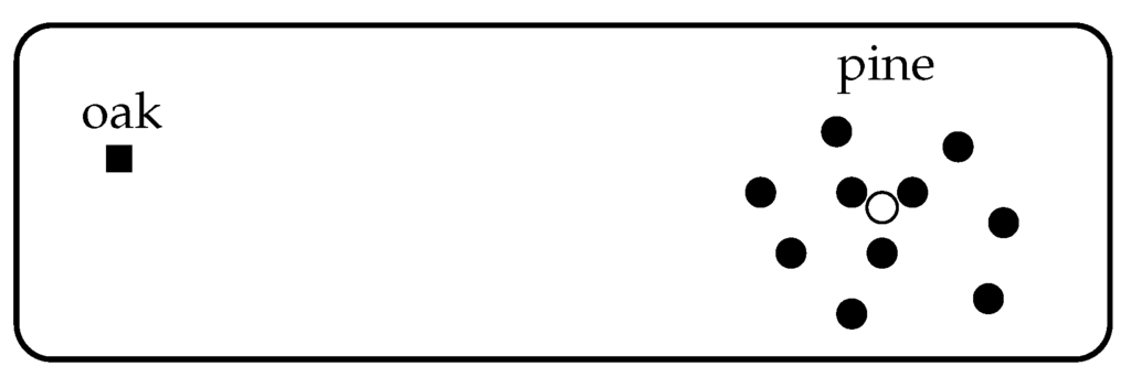
We argue that it is. Consider, for instance, a forest consisting of one species of oak and ten species of pine, with each species equally abundant. Suppose that an eleventh species of pine is added, again with equal abundance (Figure 4). This makes the forest even more heavily dominated by pine, so it is intuitively reasonable that the diversity should decrease. But now running time backwards, the conclusion is that if we start with a forest containing the oak and all eleven pine species, eliminating the eleventh should increase diversity.

Figure 4. Hypothetical community consisting of one species of oak (▪) and ten species of pine (•), to which one further species of pine is then added (◦). Distances between species indicate degrees of dissimilarity (not to scale).

To clarify further, recall from Section 3 that diversity is defined in terms of the relative abundances only. Thus, eliminating species i causes not only a decrease in $p_i$, but also an increase in the other relative abundances $p_j$. If the i-th species is particularly ordinary within the community (like the eleventh species of pine), then eliminating it makes way for less ordinary species, resulting in a more diverse community.

The instinct that maximizing diversity should not eliminate any species is based on the assumption that the distinction between species is of high value. (After all, if two species were very nearly identical—or in the extreme, actually identical—then losing one would be of little importance.) If one wishes to make that assumption, one must build it into the model. This is done by choosing a similarity matrix $\mathbf{Z}$ with a low similarity coefficient $Z_{ij}$ for each $i\ne j$. Thus, $\mathbf{Z}$ is close to the identity matrix $\mathbf{I}$ (assuming that similarity is measured on a scale of 0 to 1). Example 14 guarantees that in this case, there is a unique maximizing distribution and it does not, in fact, eliminate any species.

(The fact that maximizing distributions can eliminate some species has previously been discussed in the ecological literature in the case $q=2$; see Pavoine and Bonsall [34] and references therein.)

We now derive necessary and sufficient conditions for a similarity matrix $\mathbf{Z}$ to admit at least one maximizing distribution of full support, and also necessary and sufficient conditions for every maximizing distribution to have full support. The latter conditions are genuinely more restrictive; for instance, if $\mathbf{Z}=\left(\begin{array}{cc}1& 1\\ 1& 1\end{array}\right)$ then some but not all maximizing distributions have full support.

Lemma 8. 

If at least one maximizing distribution for $\mathbf{Z}$ has full support then $\mathbf{Z}$ is positive semidefinite and admits a positive weighting. Moreover, if every maximizing distribution for $\mathbf{Z}$ has full support then $\mathbf{Z}$ is positive definite.

Proof. 

Fix a maximizing distribution $\mathbf{p}$ of full support. Maximizing distributions are invariant (Corollary 1), so by (i) $\underset{\hspace{1em}\hspace{1em}}{\Rightarrow }$ (iii) of Lemma 3, $\left|\mathbf{Z}\right|\mathbf{p}$ is a weighting of $\mathbf{Z}$ and $\left|\mathbf{Z}\right|>0$. In particular, $\mathbf{Z}$ has a positive weighting.

Now we imitate the proof of Proposition 3B of [22]. For each $\mathbf{s}\in {\mathbb{R}}^n$ such that ${\sum }_{i=1}^n{s}_i=0$, define a function $f_{\mathbf{s}}:\mathbb{R}\to \mathbb{R}$ by

$$f_{\mathbf{s}}\left(t\right)={(\mathbf{p}+t\mathbf{s})}^T\mathbf{Z}(\mathbf{p}+t\mathbf{s}).$$

Using the symmetry of $\mathbf{Z}$ and the fact that $\left|\mathbf{Z}\right|\mathbf{p}$ is a weighting, we obtain

$$\begin{array}{cc}\hfill f_{\mathbf{s}}\left(t\right)& ={\mathbf{p}}^T\mathbf{Z}\mathbf{p}+2{\mathbf{s}}^T\mathbf{Z}\mathbf{p}·t+{\mathbf{s}}^T\mathbf{Z}\mathbf{s}·t^2\hfill \\ & =1/\left|\mathbf{Z}\right|+{\mathbf{s}}^T\mathbf{Z}\mathbf{s}·t^2.\hfill \end{array}$$

(20)

Now $\sum s_i=0$ and $\mathbf{p}$ has full support, so $\mathbf{p}+t\mathbf{s}\in {\Delta }_n$ for all real t sufficiently close to zero. But $f_{\mathbf{s}}\left(t\right)=1/{}^2{D}^{\mathbf{Z}}(\mathbf{p}+t\mathbf{s})$ for such t, so $f_{\mathbf{s}}$ has a local minimum at 0. Hence ${\mathbf{s}}^T\mathbf{Z}\mathbf{s}\ge 0$. It follows that $f_{\mathbf{s}}$ is everywhere positive.

We have shown that ${\mathbf{s}}^T\mathbf{Z}\mathbf{s}\ge 0$ whenever $\mathbf{s}\in {\mathbb{R}}^n$ with $\sum s_i=0$. Now take $\mathbf{x}\in {\mathbb{R}}^n$ with $\sum x_i\ne 0$. Put $\mathbf{s}=\mathbf{x}/\left(\sum x_i\right)-\mathbf{p}$. Then $\sum s_i=0$, and

$${\mathbf{x}}^T\mathbf{Z}\mathbf{x}={\left(\sum x_i\right)}^2{f}_{\mathbf{s}}\left(1\right)>0.$$

(21)

Hence $\mathbf{Z}$ is positive semidefinite.

For “moreover”, assume that every maximizing distribution for $\mathbf{Z}$ has full support. By (21), we need only show that ${\mathbf{s}}^T\mathbf{Z}\mathbf{s}>0$ whenever $\mathbf{s}\ne \mathbf{0}$ with $\sum s_i=0$. Given such an $\mathbf{s}$, choose $t\in \mathbb{R}$ such that $\mathbf{p}+t\mathbf{s}$ lies on the boundary of ${\Delta }_n$. Then $\mathbf{p}+t\mathbf{s}$ does not have full support, so is not maximizing, so does not maximize ${}^2{D}^{\mathbf{Z}}$ (by Corollary 2). Hence $f_{\mathbf{s}}\left(t\right)>f_{\mathbf{s}}\left(0\right)$, which by (20) implies that ${\mathbf{s}}^T\mathbf{Z}\mathbf{s}>0$. ☐

We can now prove the two main results of this section.

Proposition 5. 

The following are equivalent:

i.

there exists a maximizing distribution for $\mathbf{Z}$ of full support;

ii.

$\mathbf{Z}$ is positive semidefinite and admits a positive weighting.

Proof. 

(i) $\underset{\hspace{1em}\hspace{1em}}{\Rightarrow }$ (ii) is the first part of Lemma 8. For the converse, assume (ii) and choose a positive weighting $\mathbf{w}$. Then $\left|\mathbf{Z}\right|>0$, so $\mathbf{p}=\mathbf{w}/\left|\mathbf{Z}\right|$ is a probability distribution of full support. We have ${}^q{D}^{\mathbf{Z}}\left(\mathbf{p}\right)=\left|\mathbf{Z}\right|$ for all q, by Lemma 3. But the computation theorem implies that $D_{\max }\left(\mathbf{Z}\right)=\left|{\mathbf{Z}}_B\right|$ for some $B\subseteq \{1,\dots ,n\}$ such that ${\mathbf{Z}}_B$ admits a weighting, so $D_{\max }\left(\mathbf{Z}\right)\le \left|\mathbf{Z}\right|$ by Lemma 7. Hence $\mathbf{p}$ is maximizing. ☐

Proposition 6. 

The following are equivalent:

i.

every maximizing distribution for $\mathbf{Z}$ has full support;

ii.

$\mathbf{Z}$ has exactly one maximizing distribution, which has full support;

iii.

$\mathbf{Z}$ is positive definite with positive weighting;

iv.

$D_{\max }\left(\mathbf{Z}\right)>D_{\max }\left({\mathbf{Z}}_B\right)$ for every nonempty proper subset B of $\{1,\dots ,n\}$.

(The weak inequality $D_{\max }\left(\mathbf{Z}\right)\ge D_{\max }\left({\mathbf{Z}}_B\right)$ holds for any $\mathbf{Z}$, by the absent species lemma (Lemma 2).)

Proof. 

(i) $\underset{\hspace{1em}\hspace{1em}}{\Rightarrow }$ (iii) and (iii) $\underset{\hspace{1em}\hspace{1em}}{\Rightarrow }$ (ii) are immediate from Lemma 8 and Proposition 3 respectively, while (ii) $\underset{\hspace{1em}\hspace{1em}}{\Rightarrow }$ (i) is trivial.

For (i) $\underset{\hspace{1em}\hspace{1em}}{\Rightarrow }$ (iv), assume (i). Let $\varnothing \ne B⫋\{1,\dots ,n\}$. Choose a maximizing distribution ${\mathbf{p}}^{\prime }$ for ${\mathbf{Z}}_B$, and denote by $\mathbf{p}$ its extension by zero to $\{1,\dots ,n\}$. Then $\mathbf{p}$ does not have full support, so there is some $q\in [0,\infty ]$ such that $\mathbf{p}$ fails to maximize ${}^q{D}^{\mathbf{Z}}$. Hence

$$D_{\max }\left({\mathbf{Z}}_B\right)={}^q{D}^{{\mathbf{Z}}_B}\left({\mathbf{p}}^{\prime }\right)={}^q{D}^{\mathbf{Z}}\left(\mathbf{p}\right)<D_{\max }\left(\mathbf{Z}\right),$$

where the second equality is by the absent species lemma.

For (iv) $\underset{\hspace{1em}\hspace{1em}}{\Rightarrow }$ (i), assume (iv). Let $\mathbf{p}$ be a maximizing distribution for $\mathbf{Z}$. Write $B=supp\left(\mathbf{p}\right)$, and denote by ${\mathbf{p}}^{\prime }$ the restriction of $\mathbf{p}$ to B. Then for any q,

$$D_{\max }\left({\mathbf{Z}}_B\right)\ge {}^q{D}^{{\mathbf{Z}}_B}\left({\mathbf{p}}^{\prime }\right)={}^q{D}^{\mathbf{Z}}\left(\mathbf{p}\right)=D_{\max }\left(\mathbf{Z}\right),$$

again by the absent species lemma. Hence by (iv), $B=\{1,\dots ,n\}$. ☐

12. Open Questions

The main theorem, the computation theorem and Corollary 2 answer all the principal questions about maximizing the diversities ${}^q{D}^{\mathbf{Z}}$. Nevertheless, certain questions remain.

First, there are computational questions. We have found two classes of matrix $\mathbf{Z}$ for which the maximum diversity and maximizing distributions can be computed in polynomial time: ultrametric matrices (Example 12) and those close to the identity matrix $\mathbf{I}$ (Example 14). Both are biologically significant. Are there other classes of similarity matrix for which the computation can be performed in less than exponential time?

Second, we may seek results on maximization of ${}^q{D}^{\mathbf{Z}}\left(\mathbf{p}\right)$ under constraints on $\mathbf{p}$. There are certainly some types of constraint under which both parts of Theorem 1 fail, for trivial reasons: if we choose two distributions $\mathbf{p}$ and ${\mathbf{p}}^{\prime }$ whose diversity profiles cross (Figure 2b) and constrain our distribution to lie in the set $\{\mathbf{p},{\mathbf{p}}^{\prime }\}$, then there is no distribution that maximizes ${}^q{D}^{\mathbf{Z}}$ for all q simultaneously, and the maximum value of ${}^q{D}^{\mathbf{Z}}$ also depends on q. But are there other types of constraint under which the main theorem still holds?

In particular, the distribution might be constrained to lie close to a given distribution $\mathbf{p}$. The question then becomes: if we start with a distribution $\mathbf{p}$ and have the resources to change it by only a given small amount, what should we do in order to maximize the diversity?

Third, there are suggestive resemblances between the theory developed here and the theory of evolutionarily stable strategies (ESSs) for matrix games (Chapter 6 of [40]), taking the payoff matrix for the game to be the dissimilarity matrix $(1-Z_{ij})$. For instance, the condition in Lemma 3(ii) that ${\left(\mathbf{Z}\mathbf{p}\right)}_i={\left(\mathbf{Z}\mathbf{p}\right)}_j$ for all $i,j\in supp\left(\mathbf{p}\right)$ appears as one of the ESS criteria in [41]; the diversity maximization algorithm of Remark 1 closely resembles the method for finding ESSs in [42]; and the positive definiteness conditions in Section 11 are related to negative definiteness conditions in the ESS literature (such as [41]). Can results on evolutionary games be translated to give new results—or improved proofs of existing results—on maximizing diversity? In particular, the evolutionary game literature contains results on local extrema of quadratic forms [43], which (for $q=2$, at least) may be useful in answering the question of constrained maximization posed in the previous paragraph.

Fourth, we have confined ourselves to considering a single, static population and its diversity. In ecological situations, what is the relationship between diversity maximization and population dynamics? This is a very broad question, but there has been work in ecology on the entropy–dynamics connection. For instance, Zhang and Harte [44] used the principle that Boltzmann entropy should be maximized to predict population dynamics under resource constraints, incorporating into their model a parameter that reflects distinguishability within species relative to distinguishability between species.

Fifth, we have seen that every symmetric matrix $\mathbf{Z}$ satisfying conditions (2) (for instance, every symmetric matrix of positive reals) has attached to it a real number, the maximum diversity $D_{\max }\left(\mathbf{Z}\right)$. What is the significance of this invariant?

We know that it is closely related to the magnitude of matrices. This has been most intensively studied in the context of metric spaces. By definition, the magnitude of a finite metric space X is the magnitude of the matrix $\mathbf{Z}={\left(e^{-d(i,j)}\right)}_{i,j\in X}$; see [13,38,45], for instance. In the metric context, the meaning of magnitude becomes clearer after one extends the definition from finite to compact spaces (which is done by approximating them by finite subspaces). Magnitude for compact metric spaces has recognizable geometric content: for example, the magnitude of a 3-dimensional ball is a cubic polynomial in its radius (Theorem 2 of [15]) and the magnitude of a homogeneous Riemannian manifold is closely related to its total scalar curvature (Theorem 11 of [17]).

Thus, it is natural to ask: can one extend Theorem 1 to some class of “infinite matrices” $\mathbf{Z}$? (For instance, $\mathbf{Z}$ might be the form $(x,y)\mapsto e^{-d(x,y)}$ arising from a compact metric space. In this case, the maximum diversity of order 2 is a kind of capacity, analogous to classical definitions in potential theory; for a compact subset of ${\mathbb{R}}^n$, it coincides with the Bessel capacity of an appropriate order [16].) And if so, what is the geometric significance of maximum diversity in that context?

There is already evidence that this is a fruitful line of enquiry. In [16], Meckes gave a definition of the maximum diversity of order 2 of a compact metric space, and used it to prove a purely geometric theorem relating magnitude to fractional dimensions of subsets of ${\mathbb{R}}^n$. If this maximum diversity can be shown to be equal to the maximum diversity of all other orders then further geometric results may come within reach.

The final question concerns interpretation. Throughout, we have interpreted ${}^q{D}^{\mathbf{Z}}\left(\mathbf{p}\right)$ in terms of ecological diversity. However, there is nothing intrinsically biological about any of our results. For example, in an information-theoretic context, the “species” might be the code symbols, with two symbols seen as similar if one is easily mistaken for the other; or if one wishes to transmit an image, the “species” might be the colours, with two colours seen as similar if one is an acceptable substitute for the other (much as in rate distortion theory [46]). Under these or other interpretations, what is the significance of the theorem that the diversities of all orders can be maximized simultaneously?

References

- Leinster, T.; Cobbold, C.A. Measuring diversity: The importance of species similarity. Ecology 2012, 93, 477–489. [Google Scholar] [CrossRef] [PubMed]
- Rao, C.R. Diversity and dissimilarity coefficients: A unified approach. Theor. Popul. Biol. 1982, 21, 24–43. [Google Scholar] [CrossRef]
- Rényi, A. On Measures of Entropy and Information. In Proceedings of the 4th Berkeley Symposium on Mathematical Statistics and Probability, Berkeley, CA, USA, 20 June–30 July 1960; University of California Press: Oakland, CA, USA, 1961; Volume 1, pp. 547–561. [Google Scholar]
- Tsallis, C. Possible generalization of Boltzmann–Gibbs statistics. J. Stat. Phys. 1988, 52, 479–487. [Google Scholar] [CrossRef]
- Patil, G.P.; Taillie, C. Diversity as a concept and its measurement. J. Am. Stat. Assoc. 1982, 77, 548–561. [Google Scholar] [CrossRef]
- Havrda, J.; Charvát, F. Quantification method of classification processes: concept of structural α-entropy. Kybernetika 1967, 3, 30–35. [Google Scholar]
- Veresoglou, S.D.; Powell, J.R.; Davison, J.; Lekberg, Y.; Rillig, M.C. The Leinster and Cobbold indices improve inferences about microbial diversity. Fungal Ecol. 2014, 11, 1–7. [Google Scholar] [CrossRef]
- Bakker, M.G.; Chaparro, J.M.; Manter, D.K.; Vivanco, J.M. Impacts of bulk soil microbial community structure on rhizosphere microbiomes of Zea mays. Plant Soil 2015, 392, 115–126. [Google Scholar] [CrossRef]
- Jeziorski, A.; Tanentzap, A.J.; Yan, N.D.; Paterson, A.M.; Palmer, M.E.; Korosi, J.B.; Rusak, J.A.; Arts, M.T.; Keller, W.; Ingram, R.; et al. The jellification of north temperate lakes. Proc. R. Soc. B 2015, 282. [Google Scholar] [CrossRef] [PubMed]
- Chalmandrier, L.; Münkemüller, T.; Lavergne, S.; Thuiller, W. Effects of species’ similarity and dominance on the functional and phylogenetic structure of a plant meta-community. Ecology 2015, 96, 143–153. [Google Scholar] [CrossRef] [PubMed]
- Bromaghin, J.F.; Rode, K.D.; Budge, S.M.; Thiemann, G.W. Distance measures and optimization spaces in quantitative fatty acid signature analysis. Ecol. Evol. 2015, 5, 1249–1262. [Google Scholar] [CrossRef] [PubMed]
- Wang, L.; Zhang, M.; Jajodia, S.; Singhal, A.; Albanese, M. Modeling Network Diversity for Evaluating the Robustness of Networks against Zero-Day Attacks. In Proceedings of the 19th European Symposium on Research in Computer Security (ESORICS 2014), Wroclaw, Poland, 7–11 September 2014; pp. 494–511.
- Leinster, T. The magnitude of metric spaces. Doc. Math. 2013, 18, 857–905. [Google Scholar]
- Leinster, T. The Euler characteristic of a category. Doc. Math. 2008, 13, 21–49. [Google Scholar]
- Barceló, J.A.; Carbery, A. On the magnitudes of compact sets in Euclidean spaces. 2015; arXiv:1507.02502. [Google Scholar]
- Meckes, M.W. Magnitude, diversity, capacities, and dimensions of metric spaces. Potential Anal. 2015, 42, 549–572. [Google Scholar] [CrossRef]
- Willerton, S. On the magnitude of spheres, surfaces and other homogeneous spaces. Geom. Dedicata 2014, 168, 291–310. [Google Scholar] [CrossRef]
- Leinster, T. The magnitude of a graph. 2014; arXiv:1401.4623. [Google Scholar]
- Hepworth, R.; Willerton, S. Categorifying the magnitude of a graph. 2015; arXiv:1505.04125. [Google Scholar]
- Chuang, J.; King, A.; Leinster, T. On the magnitude of a finite dimensional algebra. Theory Appl. Categories 2016, 31, 63–72. [Google Scholar]
- Leinster, T. A maximum entropy theorem with applications to the measurement of biodiversity. 2009; arXiv:0910.0906. [Google Scholar]
- Fremlin, D.H.; Talagrand, M. Subgraphs of random graphs. Trans. Am. Math. Soc. 1985, 291, 551–582. [Google Scholar] [CrossRef]
- Simpson, E.H. Measurement of diversity. Nature 1949, 163, 688. [Google Scholar] [CrossRef]
- Whittaker, R.H. Vegetation of the Siskiyou mountains, Oregon and California. Ecol. Monogr. 1960, 30, 279–338. [Google Scholar] [CrossRef]
- Magurran, A.E. Measuring Biological Diversity; Wiley-Blackwell: Hoboken, NJ, USA, 2003. [Google Scholar]
- Hurlbert, S.H. The nonconcept of species diversity: A critique and alternative parameters. Ecology 1971, 52, 577–586. [Google Scholar] [CrossRef]
- Kimura, M.; Crow, J.F. The number of alleles that can be maintained in a finite population. Genetics 1964, 49, 725–738. [Google Scholar] [PubMed]
- Hannah, L.; Kay, J.A. Concentration in the Modern Industry: Theory, Measurement, and the U.K. Experience; MacMillan: London, UK, 1977. [Google Scholar]
- McBratney, A.; Minasny, B. On measuring pedodiversity. Geoderma 2007, 141, 149–154. [Google Scholar] [CrossRef]
- Hardy, G.H.; Littlewood, J.E.; Pólya, G. Inequalities, 2nd ed.; Cambridge University Press: Cambridge, UK, 1952. [Google Scholar]
- Chao, A.; Chiu, C.H.; Jost, L. Phylogenetic diversity measures based on Hill numbers. Philos. Trans. R. Soc. B 2010, 365, 3599–3609. [Google Scholar] [CrossRef] [PubMed]
- Lawvere, F.W. Metric spaces, generalized logic and closed categories. Rendiconti del Seminario Matematico e Fisico di Milano 1973, 43, 135–166, reprinted in Repr. Theory Appl. Categories 2002, 1, 1–37. [Google Scholar] [CrossRef]
- Gromov, M. Metric Structures for Riemannian and Non-Riemannian Spaces; Birkhäuser: Boston, MA, USA, 2001. [Google Scholar]
- Pavoine, S.; Bonsall, M.B. Biological diversity: distinct distributions can lead to the maximization of Rao’s quadratic entropy. Theor. Popul. Biol. 2009, 75, 153–163. [Google Scholar] [CrossRef] [PubMed]
- Kolmogorov, A.N. On certain asymptotic characteristics of completely bounded metric spaces. Doklady Akademii Nauk SSSR 1956, 108, 385–388. [Google Scholar]
- Berarducci, A.; Majer, P.; Novaga, M. Infinite paths and cliques in random graphs. Fundam. Math. 2012, 216, 163–191. [Google Scholar] [CrossRef]
- Karp, R.M. Reducibility among Combinatorial Problems. In Complexity of Computer Computations; Miller, R.E., Thatcher, J.W., Eds.; Plenum Press: New York, NY, USA, 1972; pp. 85–103. [Google Scholar]
- Meckes, M.W. Positive definite metric spaces. Positivity 2013, 17, 733–757. [Google Scholar] [CrossRef]
- Horn, R.A.; Johnson, C.R. Matrix Analysis, 2nd ed.; Cambridge University Press: Cambridge, UK, 2012. [Google Scholar]
- Broom, M.; Rychtář, J. Game-Theoretical Models in Biology; Chapman & Hall/CRC Press: Boca Raton, FL, USA, 2013. [Google Scholar]
- Haigh, J. Game theory and evolution. Adv. Appl. Probab. 1975, 7, 8–11. [Google Scholar] [CrossRef]
- Bishop, D.T.; Cannings, C. Models of animal conflict. Adv. Appl. Probab. 1976, 8, 616–621. [Google Scholar] [CrossRef]
- Broom, M.; Cannings, C.; Vickers, G.T. On the number of local maxima of a constrained quadratic form. Proc. R. Soc. A 1993, 443, 573–584. [Google Scholar] [CrossRef]
- Zhang, Y.J.; Harte, J. Population dynamics and competitive outcome derive from resource allocation statistics: The governing influence of the distinguishability of individuals. Theor. Popul. Biol. 2015, 105, 53–63. [Google Scholar] [CrossRef] [PubMed]
- Leinster, T.; Willerton, S. On the asymptotic magnitude of subsets of Euclidean space. Geom. Dedicata 2013, 164, 287–310. [Google Scholar] [CrossRef]
- Cover, T.M.; Thomas, J.A. Elements of Information Theory; Wiley: New York, NY, USA, 1991. [Google Scholar]
© 2016 by the authors; licensee MDPI, Basel, Switzerland. This article is an open access article distributed under the terms and conditions of the Creative Commons by Attribution (CC-BY) license (http://creativecommons.org/licenses/by/4.0/).