Article

Wavelet Entropy-Based Traction Inverter Open Switch Fault Diagnosis in High-Speed Railways

1
Key Laboratory of Magnetic Suspension Technology and Maglev Vehicle, Ministry of Education, Southwest Jiaotong University, Chengdu 610031, China
2
School of Electrical Engineering, Southwest Jiaotong University, Chengdu 610031, China
*
Author to whom correspondence should be addressed.
Entropy 2016, 18(3), 78; https://doi.org/10.3390/e18030078
Submission received: 18 December 2015 / Revised: 28 January 2016 / Accepted: 17 February 2016 / Published: 1 March 2016
(This article belongs to the Special Issue Wavelets, Fractals and Information Theory I)

Abstract

:
In this paper, a diagnosis plan is proposed to settle the detection and isolation problem of open switch faults in high-speed railway traction system traction inverters. Five entropy forms are discussed and compared with the traditional fault detection methods, namely, discrete wavelet transform and discrete wavelet packet transform. The traditional fault detection methods cannot efficiently detect the open switch faults in traction inverters because of the low resolution or the sudden change of the current. The performances of Wavelet Packet Energy Shannon Entropy (WPESE), Wavelet Packet Energy Tsallis Entropy (WPETE) with different non-extensive parameters, Wavelet Packet Energy Shannon Entropy with a specific sub-band (WPESE3,6), Empirical Mode Decomposition Shannon Entropy (EMDESE), and Empirical Mode Decomposition Tsallis Entropy (EMDETE) with non-extensive parameters in detecting the open switch fault are evaluated by the evaluation parameter. Comparison experiments are carried out to select the best entropy form for the traction inverter open switch fault detection. In addition, the DC component is adopted to isolate the failure Isolated Gate Bipolar Transistor (IGBT). The simulation experiments show that the proposed plan can diagnose single and simultaneous open switch faults correctly and timely.

1. Introduction

Vector controlled drive systems are widely adopted in the high-speed railways of China. In this kind of drive system, the traction inverters are essential to meet the control demand. However, the traction inverters are prone to suffer failures because of their complex working environment and exposure to high stress [1]. These failures threaten the train’s operational safety. Fortunately, a fault tolerant strategy, which requires the timely and correct diagnosis of traction inverter failures, is a feasible way to avoid this risk [2,3].
An earlier survey has pointed out that semiconductor power devices (SPDs) ranked among the most fragile components in power electronic converters [4]. SPD failures include open switch faults and short switch faults. The short switch faults will cause an intense increase of the load current. As a result, the time between fault initiation and failure is very short, which makes it difficult to execute diagnosis algorithms. Hence, the existing short switch fault diagnosis methods are almost always based on hardware [5]. As for the open switch faults, the system can still run for a while, which may cause additional failures and damage the system. Therefore, it is important to diagnose open switch faults in time.
Recently, numerous methods for the fault diagnosis of SPDs failures have been proposed [6,7,8,9,10,11,12,13,14,15,16,17,18,19]. These methods can mainly be divided into model-based approaches [6,7,8,9] and signal-based approaches [10,11,12,13,14,15,16,17,18,19]. Generally, the model-based approaches perform the diagnosis by generating the residuals which will not exceed the threshold unless the failures occur. In [6], the residuals were defined as the difference between the theoretical voltage and actual voltage across each SPD. In addition, the hardware was adopted to decrease the sensors. However, the cost would increase compared with [7,8,9]. In [7], robust residuals were constructed by combining two nonlinear Luenberger observers with a directional evaluation. The residuals could identify the fault bridge and the directional value can locate the failure SPD. In [8], a residual, which had robustness against false alarms, was constructed by employing a voltage observer, coupled with the DC voltage. The diagnosing rule was similar to [7]. In [9], a model-based approach based on the cross correlation between the estimated phase currents by a sliding mode observer and the real currents was proposed.
Signal-based approaches are mainly based on the output current or voltage of the inverter. The average values and average absolute values of stator currents were adopted as principal quantities to formulate the diagnostic variables [10,11]. The Concordia current pattern could also detect the open switch fault and identify the failure SPD [12]. Extra component analysis, averaging, and waveform analysis were adopted in [13] to identify the failure SPD. In [14], a discrete wavelet transform was utilized to detect SPD failures. Then the value and the polarity of DC offset of each phase current were fed to a fuzzy logic system to isolate the failed SPD. Multi-resolution based on wavelet transform was performed in [15,16], and the features of open switch faults were discussed. However, it was argued in [17] that a sudden change of current amplitude by transient states was the obstacle in performing fault diagnosis by wavelet transform, and the normalized form of each phase was adopted. However, this form would change the waveform of the fault-free phase currents, which made it difficult to diagnose the simultaneous faults. In [18,19], the numerical values of wavelet coefficients were adopted instead of the waveform, and improved support vector machines were proposed to classify the faults.
Based on the above discussion, it can be found that the wavelet transform may not be a good method to deal with traction inverter open switch faults. On one hand, the sudden change of current amplitude by transient states will cause false alarms, and the current contains higher extra components that may cover the fault signal. On the other hand, if any measure is adopted to deal with the phenomenon mentioned above, the fault-free phase currents might be influenced at the same time, which makes it hard to diagnose the simultaneous faults.
Recently, entropy has shown outstanding performance in the fault detection domain [20,21,22,23]. In [20], multi-wavelet singular entropies were proposed to detect and classify faults in power transmission lines. In [21,22], wavelet singular entropy and relative entropy of wavelet energy were utilized in power system protection applications. In [23], multi-level wavelet Shannon entropy was proposed to isolate single-sensor faults.
Considering the ability of entropy in fault detection, a plan for traction inverter open switch fault diagnosis based on wavelet packet entropy is proposed in this paper. This plan mainly consists of two parts, namely, the fault detection part and the fault location part. For the fault detection part, five entropy forms, i.e., Wavelet Packet Energy Shannon Entropy (WPESE), Wavelet Packet Energy Tsallis Entropy (WPETE) with different non-extensive parameters, Empirical Mode Decomposition Shannon Entropy (EMDESE), Wavelet Packet Energy Shannon Entropy with a specific sub-band (WPESE3,6) and Empirical Mode Decomposition Tsallis Entropy (EMDETE) with different parameters are tried to overcome the defects of the traditional fault detection methods. For the fault isolation part, the DC component of each faulty leg is calculated to identify the Upper Switch Fault (USF) and Lower Switch Fault (LSF). Finally, simulation experiments are performed to validate the effectiveness of the proposed methodology.

2. Disadvantages of Wavelet and Wavelet Packet in Traction Inverter Diagnosis

The schematic diagram of traction system is shown in Figure 1. The traction inverter mainly consists of six SPDs, namely S1, S2, S3, S4, S5, S6. Insulated Gate Bipolar Transistors (IGBTs) with antiparallel diodes are commonly adopted SPDs [7]. In the traction system, the vector control is utilized to decouple the excitation current and torque current. Hence, it can be easier to control the motor’s torque. The A-phase current and motor’s torque under normal condition and S1 open switch fault condition are shown in Figure 2, respectively. It can be found that the open switch fault will cause a sudden change of the torque, which may damage the traction motor and may threaten the passengers’ safety.
With high order vanishing moments wavelets, the detail wavelet decomposition coefficients will become small. When a singularity occurs, the detail coefficients will become large. This characteristic makes it possible for the Discrete Wavelet Transform (DWT) and Discrete Wavelet Packet Transform (DWPT) to detect the open switch faults in traction inverters. In this section, the performances of DWT and DWPT in diagnosing open switch faults in traction inverters are evaluated.

2.1. Disadvantages of Wavelet Transform

DWT, which has multi-resolution analysis ability, can decompose the signal into different scales by utilizing the orthogonal wavelet basis as Equation (1) shows:
f ( t ) = k a m ( k ) φ ( t k ) + k j c j 2 j / 2 ψ ( 2 j t k ) ,       j = 1 , 2 , ... , m
where, f ( t ) is the original signal, φ ( t ) is the scaling function, ψ ( t ) is the wavelet function, a m represents the last scale approximate coefficient and cj is the detail coefficients in jth scale. By this equation, the time domain signal can be mapped into different scales, or the frequency domain in some way. This process can be expressed as shown in Figure 3. In the first level, the original signal is decomposed into high frequency sub-band D1 and low frequency sub-band A1. In the second level, the low frequency sub-band A1 is composed into high sub-band D2 and low frequency sub-band A2, as well as in the later levels.
To evaluate the performance of the DWT, db2 wavelet is adopted as recommended by [17]. Figure 4 shows the A-phase fault current with S1 open and the results of db2 wavelet decomposition with a 50 kHz sampling rate. From the detail coefficients, it is hard to detect the open switch fault. As shown in Figure 5, it is clear that the fault-free current contains the main components at the frequencies of 60, 360, 640, 920 and 1050 Hz. The fundamental frequency is 60 Hz, and the components at other frequencies are called extra components. After the S1 open fault occurs, extra components appear around 0 and 130 Hz frequency. The frequency range of each sub-band can be presented as Equation (2):
{ D j : [ 2 j f max , 2 j + 1 f max ] A j : [ 0 , 2 j f max ]       j = 1 , 2 , ... , m
where, fmax represents the frequency of the highest component. Hence, the frequency range of each sub-band can be obtained as shown in Table 1. Sub-band D1 contains the extra components of 640 and 920 Hz, sub-band D2 contains the extra components of 360 Hz, sub-band D3 contains the extra components around 130 Hz. As each sub-band contains the extra components of the fault current, the fault signal is covered by the extra components in each sub-band, which makes it difficult to detect the switch open faults.

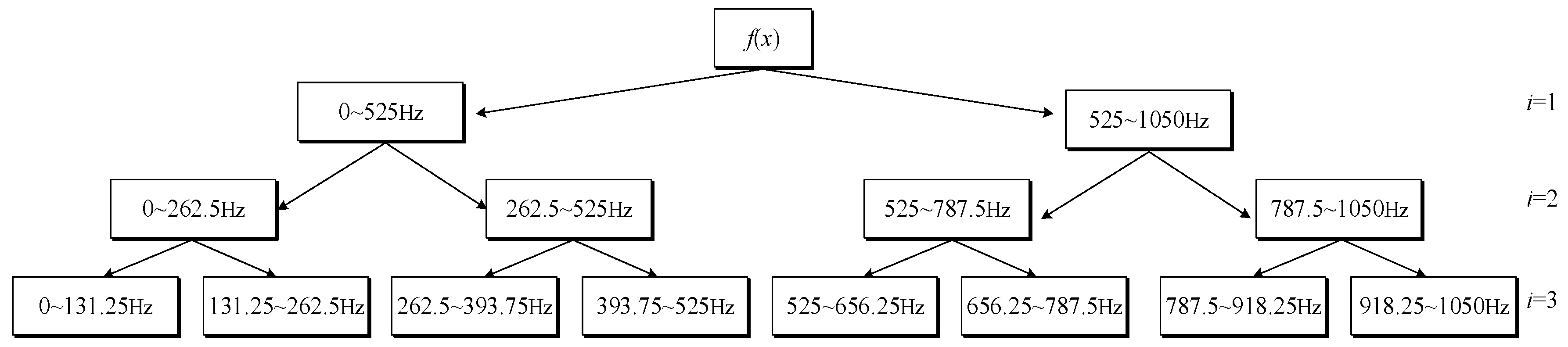
2.2. Disadvantages of Discreet Wavelet Packet Transform

As shown in Figure 3, DWT can decompose the approximate part in each level, while the detail part remains unchanged. Consequently, the resolution of DWT is not high enough to separate the fault signals from the extra components. Differing from DWT, DWPT can decompose the detail part in each level. Hence, its resolution may be high enough to detect the open switch faults. DWPT recursive decomposition can be expressed as follows:
{ d i , 2 j ( t ) = 2 k g ( k ) d i 1 , j ( 2 t k ) d i , 2 j 1 ( t ) = 2 k h ( k ) d i 1 , j ( 2 t k ) d 0 , 0 ( t ) = f ( x ) ( t )
where, f(x) represents the original signal, h(k) and g(k) are the high pass filter and low pass filter respectively, and di,j(k) is the reconstructed signal of wavelet packet decomposition for the jth node at the ith level. In this part, db2 wavelet is selected as the mother wavelet as well and Shannon entropy is adopted to search for the best wavelet packet base. In order to eliminate the effects of extra components, the high frequency sub-band that does not contain any extra component should be selected to detect the open switch faults. The frequency of each sub-band after wavelet packet decomposition is depicted in Figure 6, and the 656.25~787.5 Hz sub-band, namely the sixth node in the third level, is selected.
Figure 7 shows the DWPT decomposition coefficients of the sixth node in the third level. The fault detection results are much better than that of the DWT, because this sub-band is not affected by the extra components owing to its high resolution in the frequency domain. However, as mentioned in the introduction, the wavelet transform or wavelet packet transform may lead to false alarms in detecting the open switch faults of traction inverters. It can be found in Figure 7 that the false alarms are caused by the sudden change of current amplitude.
In this section, the performances of DWT and DWPT in diagnosing the open switch faults in traction inverters are discussed. Neither DWT nor DWPT can detect the open switch faults in traction inverters ideally, though it is possible for DWT and DWPT to detect singularities. The output currents of the traction inverter, namely the stator currents, contain the high frequency extra components both under normal conditions and fault conditions. As the resolution of DWT is not so satisfying in the high frequency domain, the extra components which fall into the high frequency sub-bands cover the fault signals. The decomposition results show that DWT can hardly detect the open switch faults. DWPT has higher resolution than DWT and it can detect the fault. Nevertheless, there is a fatal problem for DWPT to detect the open switch faults. That is to say, the sudden change of the current will lead to the false alarms, hence the detection results are not reliable. Though some measures can be implemented to eliminate the false alarms, they will change the waveform of other phase currents and cause alarms in the fault-free phase, which makes it more difficult to diagnose the simultaneous faults. If this disadvantage of DWPT can be solved, the open switch fault can be detected in a timely way and correctly.

3. Proposed Diagnosis Plan

In order to overcome the defects of DWT and DWPT in traction inverter diagnosis, a new plan is proposed. First, the entropy approach is adopted to detect the open switch faults. Five entropy forms, namely, WPESE, WPETE, WPESE3,6, EMDESE and EMDETE, are tried and discussed. With the evaluation parameter, the best entropy form that can deal with the false alarms in this case is found. Then, the DC component of the faulty phase current is considered to locate USF and LSF.

3.1. Fault Detection Method

3.1.1. Wavelet Packet Shannon Entropy and Tsallis Entropy

Entropy can measure the uncertainty of a system. It has been discussed in Section 2 that the fault current has more frequency components than normal current. As a result, the entropy in a fault case is larger than that of a normal case. Hence, Shannon entropy and Tsallis entropy are utilized to detect the faults.
Shannon entropy was firstly proposed by Shannon to solve the measurement problem of information. Supposing a random variable X ( X = x 1 , x 2 , ... , x N , N is the number of probable states) as the state of an uncertain system, the information of one state can be expressed by Equation (4) and the Shannon entropy can be presented as Equation (5):
I j = log ( 1 / p j )
H ( X ) = j = 1 N p j log ( p j )
where pj is the probability of xi, and the sum of pj is equal to 1.
By DWPT, Di,j(n) (n = 1, 2, … , K) is set as the reconstructed signal of the ith node at the jth level, n is the index of sampling point. The Wavelet Packet Energy (WPE) of each node at jth level can be expressed as Equation (6), and the total energy of the signal Ej is the sum of WPE of every node. Relative wavelet packet energy pi,j = Ei,j/Ej can be treated as the probability. Hence, the Wavelet Packet Energy Shannon Entropy (WPESE) at jth level can be defined as Equation (7):
E i , j = n = 1 k | D i , j ( n ) | 2
W P E S E = i = 1 J p i , j log p i , j , ( J = 2 j )
Shannon entropy is a kind of extensive entropy, i.e., it is used for the additive system. Tsallis entropy is one of the non-extensive entropies that can provide the correct physical expression for the non-additive system with a mixed or irregular fragment [21]. The expression of Wavelet Packet Energy Tsallis Entropy (WPETE) is defined as Equation (8):
W P E T E = 1 q 1 ( 1 i = 1 J ( p i , j ) q ) ,   ( J = 2 j )
where, q represents the non-extensive parameter, the meanings of the rest variables are similar to those in Equation (7).
The non-extensive parameter q plays an important role in Tsallis entropy. When q approaches 0, Tsallis entropy and Shannon entropy are equal, which means the Tsallis entropy is extensive in this occasion. For the wavelet packet decomposition, the coefficients in each scale are generally non-extensive because of the frequency aliasing and energy leakage. Hence, it should be considered carefully. In this paper, q in the range of [0.1,0.9] and [2,9] is considered respectively.
The performances of WPESE and WPETE with different q values for the open switch fault detection problem are shown in Figure 8 and Figure 9. It can be found that the WPESE still has false alarms. However, if the threshold and non-extensive parameter q is set properly, the WPETEs may be able to deal with these false alarms.

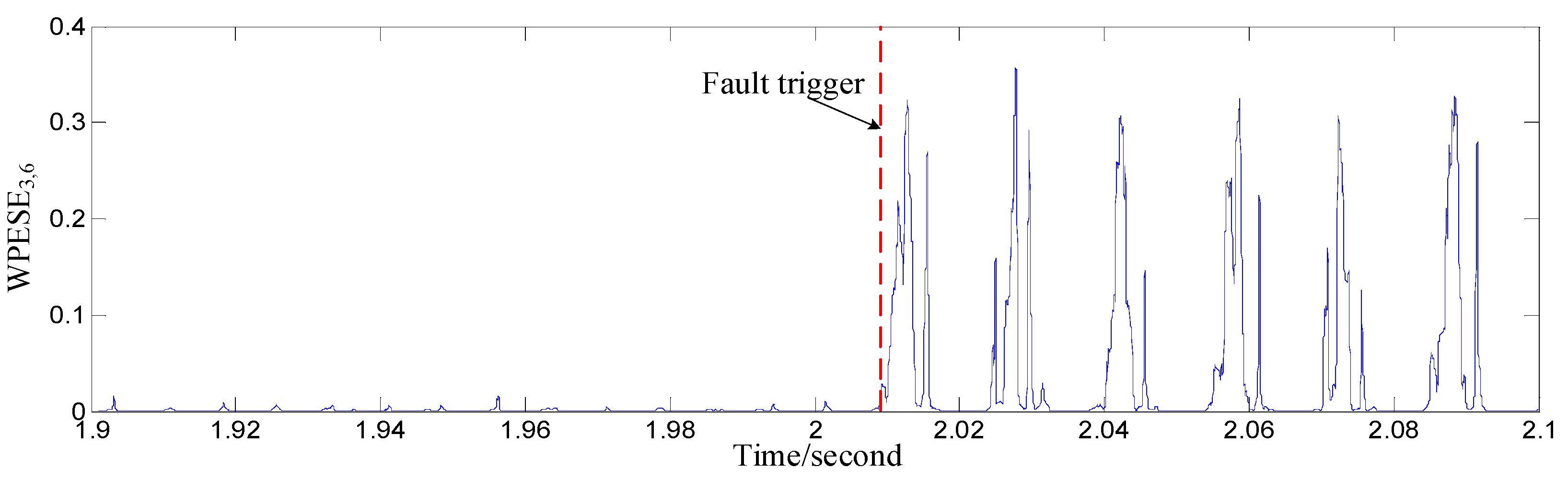
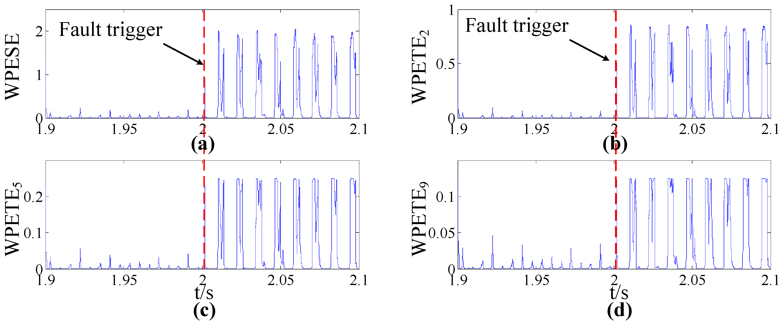
3.1.2. WPESE with a Specific Sub-Band

In Section 3.1.1, the performances of WPESE and WPETE with different non-extensive parameters q have been discussed. It can be found that both of them are still under the risk of false alarms, especially WPESE. The WPETE can be better if the non-extensive parameter is selected well because the system is non-extensive as discussed in Section 3.1.1. The reason for the false alarms is that all the sub-bands are used for the entropy calculation, which means all the extra components are considered. Hence, the entropy can be very large under the normal condition. However, if the specific sub-band that does not contain any extra component is selected to calculate the entropy, the false alarms may be eliminated.
It has been proved in Section 2.2 that the sixth node in the third level of db2 wavelet packet decomposition has no extra components if frequency aliasing and energy leakage are ignored. Therefore, this node may be able to deal with the false alarms. Adopting the concept of Shannon entropy, the WPESE of the specific sub-band (WPESE3,6) is defined as Equation (9):
W P E S E 3 , 6 = p 3 , 6 log p 3 , 6
Note that, there is only one unit in this system and Tsallis entropy is needless. From the definition of WPEE3,6, it can be found that, the node’s entropy will maintain large value during the occurrence of the fault and approach zero in other conditions. The performance of WPESE3,6 is shown in Figure 10.
As the energy calculation is based on a period of signal, a sliding window L and sliding factor a will be needed for the fault detection. The length of the window should not be too long nor too short. A long window will increase the computational cost, as well as the detection time. Short windows may lead to a decrease of detection performance. Similarly, a small sliding factor can reduce the lag between the fault trigger and fault detection. However, the computation will be raised. Hence, both of the parameters should be selected carefully. In Section 3.1.1 and Section 3.1.2, L = 50 sampling points and a = 1 sampling points are selected. Note that, the L and a selection is based on experience which makes the calculation time as short as possible under the premise of not losing the accuracy.

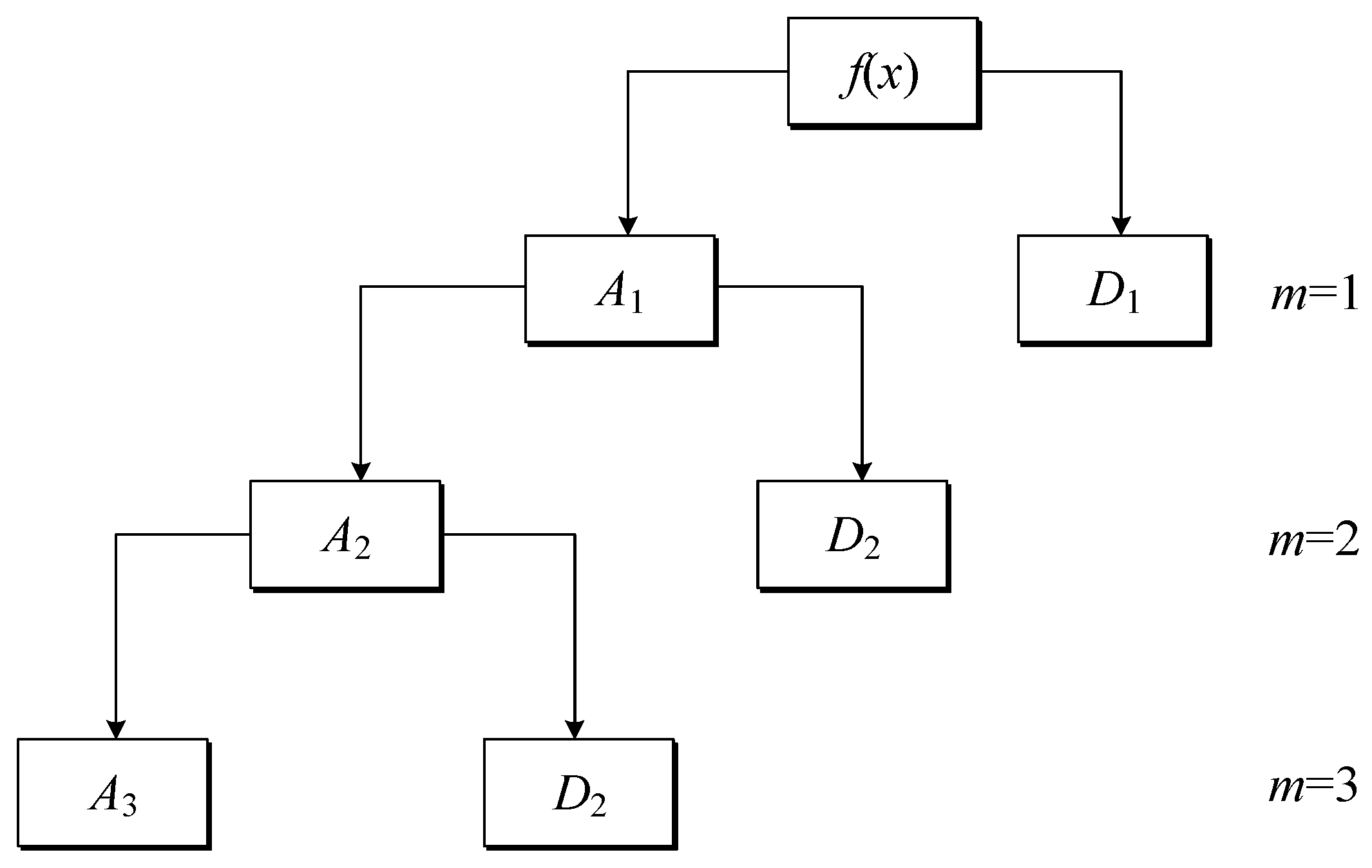
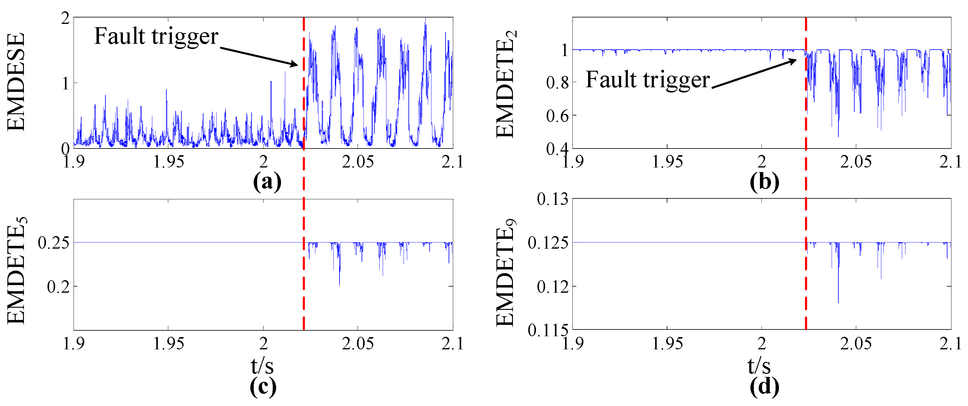
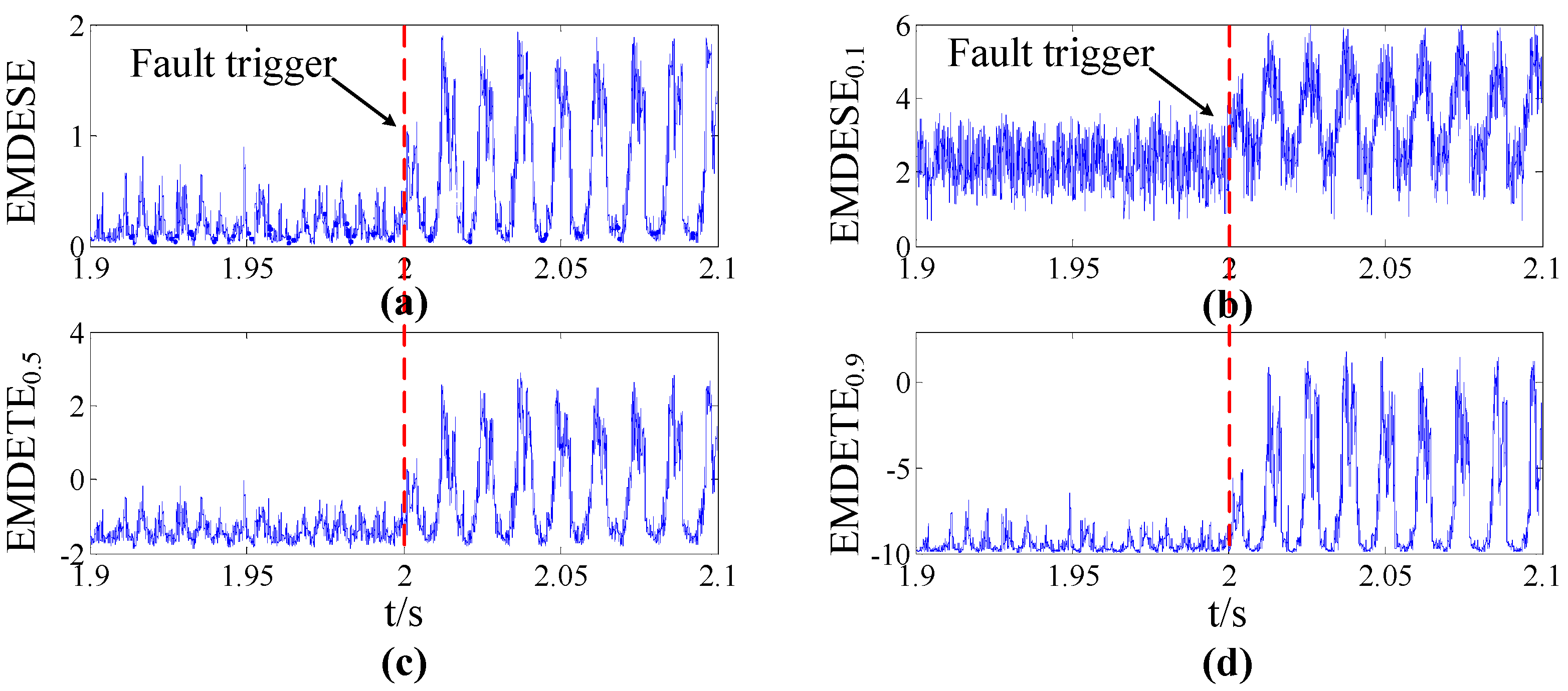
3.1.3. Empirical Mode Decomposition Shannon Entropy and Tsallis Entropy

Good diagnosis performances of EMD are reported in [24,25]. In this section, EMD and EMD entropy are introduced and utilized to detect the open switch fault. Essentially speaking, the EMD method is a kind of smoothing process, which separates the different scale signals to generate several series. Each series is called an IMF, which must satisfy the following constraints [26]:
(1)
In the whole data set, the number of extrema and the number of zero-crossings must either be equal or differ at most by one.
(2)
At any point, the mean value of the envelope defined by local maxima and the envelope defined by the local minima is zero.
The EMD method can be implemented by the following steps:
(1)
Determine all the local extrema of the original signal.
(2)
Connect all the local maxima and minima with cubic spline line, respectively. Thus, the upper envelope and lower envelop can be obtained.
(3)
Denote the average value of upper and lower envelop as m1(t), and denote:
h 1 ( t ) = f ( x , t ) m 1 ( t )
(4)
If h1(t) satisfies the constraints of IMF, then it is the first IMF of the original signal f(x,t). Else let f(x,t) = h1(t), and repeat the Steps (1)–(3) until h1(k-1)(t) − m1k(t) = h1k(t) (k is the iteration number), which means h1k(t) satisfies the IMF constraints. Denote c1(t) = h1k(t), c1(t)is the first IMF of the original signal.
(5)
Separate c1(t) from f(x,t), we can obtain the residual:
r 1 ( t ) = f ( x , t ) c 1 ( t )
Let r1(t) be the original signal, repeat the Steps (1)–(4), the second IMF c2(t) can be obtained.
(6)
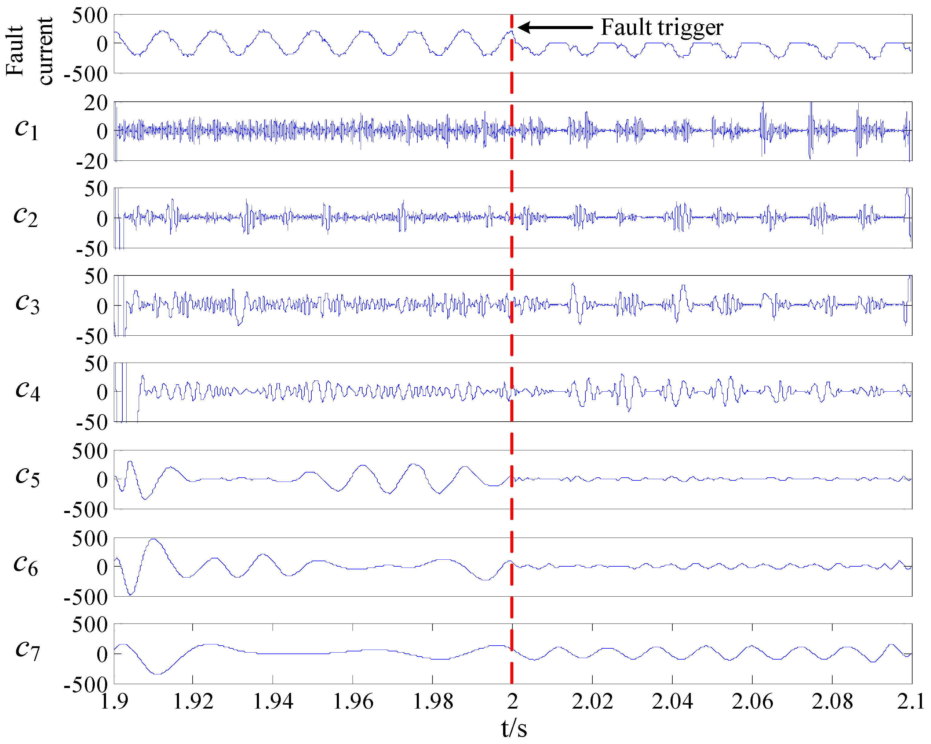
Repeat the steps above until the residual is monotonous, all the IMFs c1(t), c2(t),…, cn(t) and the final residual rn(t) can be obtained. The original signal can be expressed as:
f ( x , t ) = i = 1 n c i ( t ) + r n ( t )
Each IMF represents a specific frequency which is with respect to the original signal f(x,t). If the f(x,t) changes, for example, affected by the noise, the specific frequency of each IMF will change as well. As a consequence, the EMD energy entropy cannot be analyzed as WPESE, i.e., it is hard to find a specific IMF to avoid the extra components. In this part, EMD energy Shannon entropy (EMDESE) and Tsallis entropy (EMDETE) are discussed, which can be expressed as Equations (13) and (14):
E M D E S E = i = 1 n p i log p i
E M D E T E = 1 q 1 ( 1 i = 1 n p i q )
where, p i = c i / j = 1 n c j , q is the non-extensive parameter, and n is the number of IMFs.
The performances of EMD, EMDESE and EMDETE with non-extensive parameter q in the range of [0.1,0.9] and [2,9] are shown in Figure 11, Figure 12 and Figure 13, respectively. It can be found from these figures that it is difficult for EMD to detect the fault, while the EMDETE can finish this if the non-extensive parameter is selected properly.
In this section, L = 150 sampling points and a = 1 sampling point.

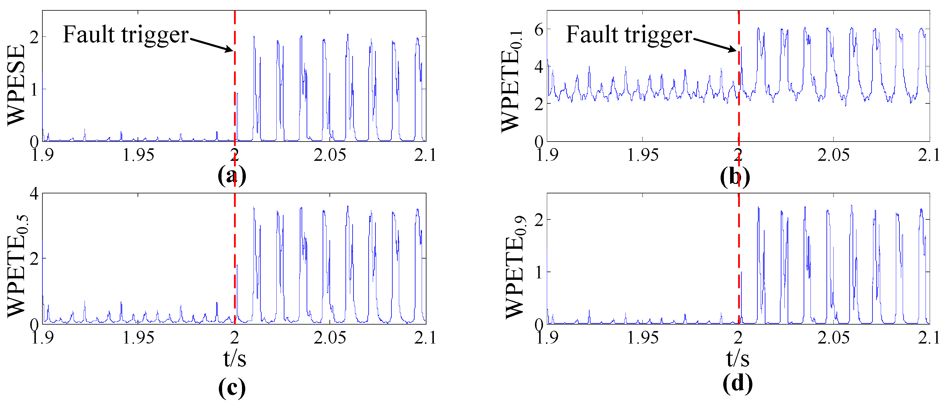
3.1.4. Fault Detection Evaluation

Earlier in this paper, the performances of WPESE, WPETE, WPESE3,6, EMDESE and EMDETE in open switch fault detection are discussed with respect to Figure 8, Figure 9, Figure 10, Figure 11, Figure 12 and Figure 13. In order to evaluate them quantitatively, the evaluation parameter is defined.
The main obstruction of open switch fault detection is the false alarms caused by the sudden changes of the current. Therefore, the maximum of the entropy in normal condition should be considered and the evaluation parameter γ is defined as follows:
γ = ln ( E n ( m a x ) E n ( m i n ) E f ( m a x ) E f ( m i n ) )
where, En(max) and En(min) represent the maximum and the minimum of the entropy under normal conditions, respectively. Ef(max) and Ef(min) indicate the maximum and the minimum of the entropy under fault conditions. From the definition of γ , it can be found that the entropy form with larger γ will be effected less by false alarms.
In order to select the most suitable non-extensive parameters q, evaluation parameter γ of each WPETE and EMDETE with different q are compared, which are shown in Figure 14.
It can be found in Figure 14 that 0.9 is the best non-extensive parameter q for WPETE and 0.5 is the best one for EMDETE. In order to select the best entropy form to detect the open switch fault, the evaluation parameter γ of each entropy form of the fault current is given in Table 2. Obviously, WPESE3,6 is the best choice in this case as it can deal with the effect of the sudden changes of the current.

3.2. DC Component and Fault Location
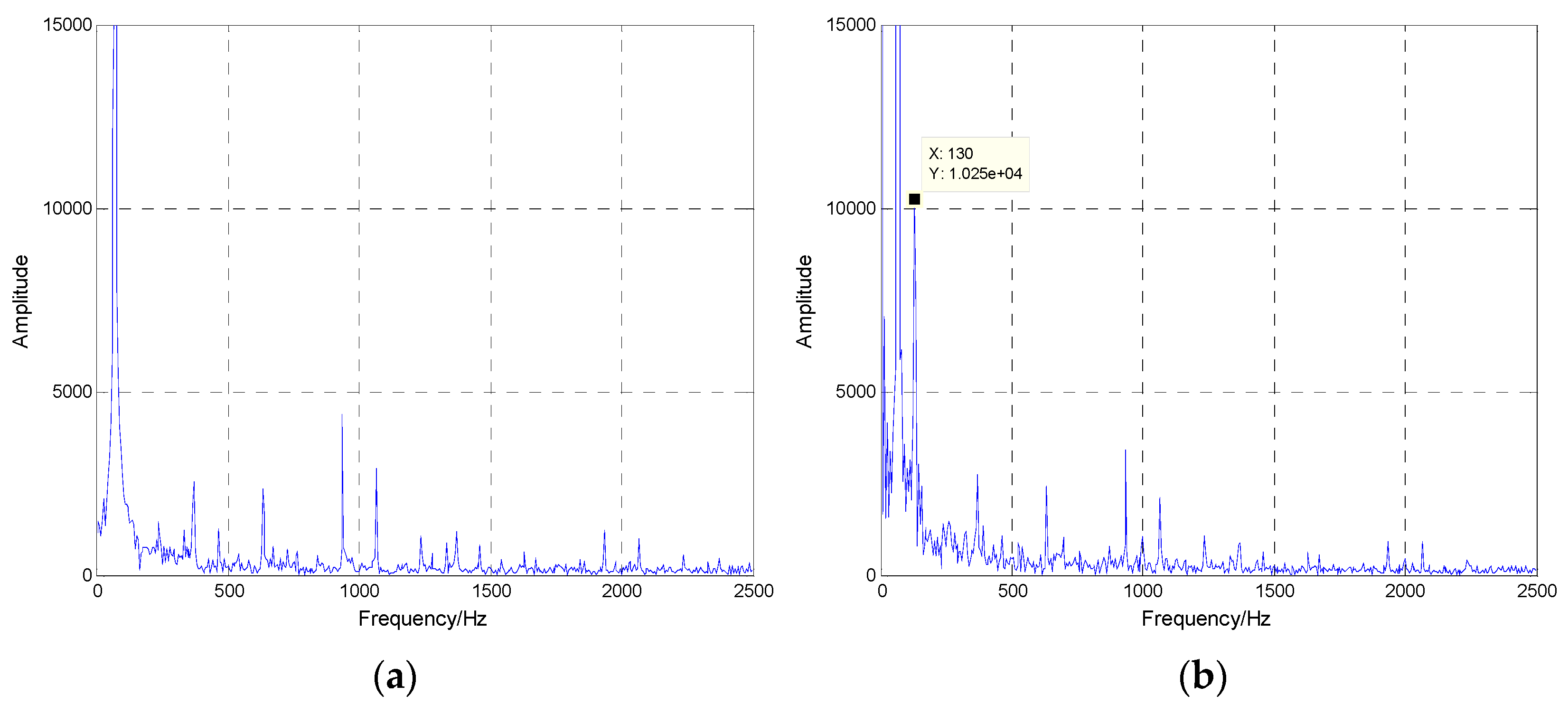
Though WPESE3,6 has shown its good performance in detecting the fault legs without false alarms, it still has problems in identifying the fault IGBT. As WPESE3,6 is calculated by the absolute value, it cannot classify the direction. Hence in this part, the DC component Idc is introduced to overcome this defect, which is depicted as Equation (16):
I d c = 1 M m = 1 M I i ( m )
where, M is the number of sampling points in one cycle, i represents the phase index.
Figure 15 shows A-phase current flows and current waves of USF and LSF. When the USF occurs, the current cannot go through S1, i.e., the positive current must be zero. However, the negative current can go through the anti-parallel diode of S4. The current wave can be seen in Figure 15b,c. If the USF occurs in the negative current flow, the current wave will remain normal until the current crosses zero. Moreover, the positive current will be replaced by zero in the next periods. If it occurs in the positive current flow, the current will approach zero immediately. Apparently, sampling points’ values of the current are almost negative after fault triggering. The analysis of LSF is similar to that of USF and the current wave is shown in the Figure 15e,f, sampling points’ values of the current are almost positive after fault triggering. From the discussion, it is clear that the DC component of the fault current will be negative after the USF, and positive after the LSF. Thus, when the fault is detected, the average value of samples during the next cycle, i.e., the DC component, can be calculated to identify the fault IGBT or IGBTs.
The open switch fault diagnosis plan can be implemented by the following steps, which is shown in the flowchart in Figure 16:
(1)
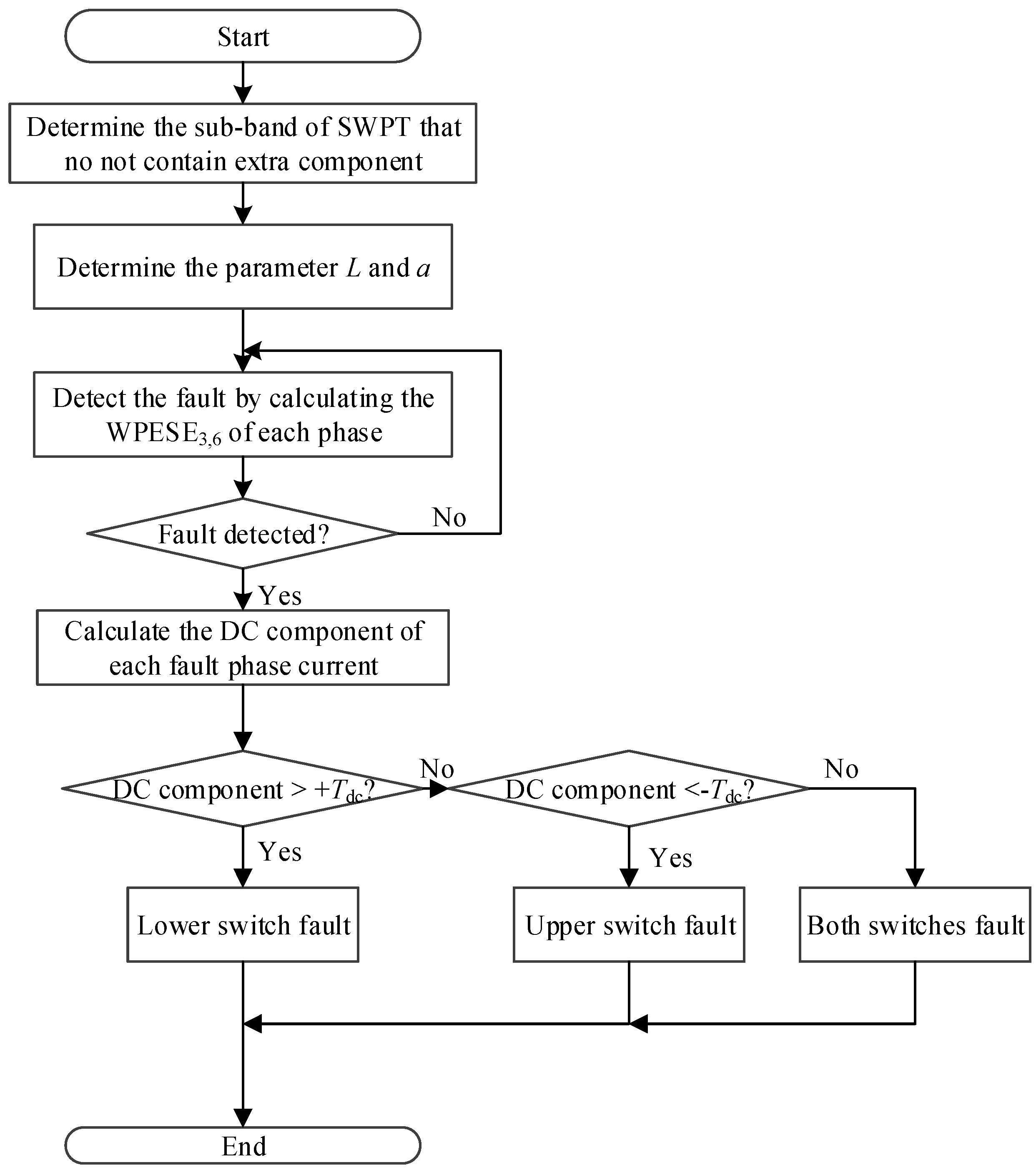
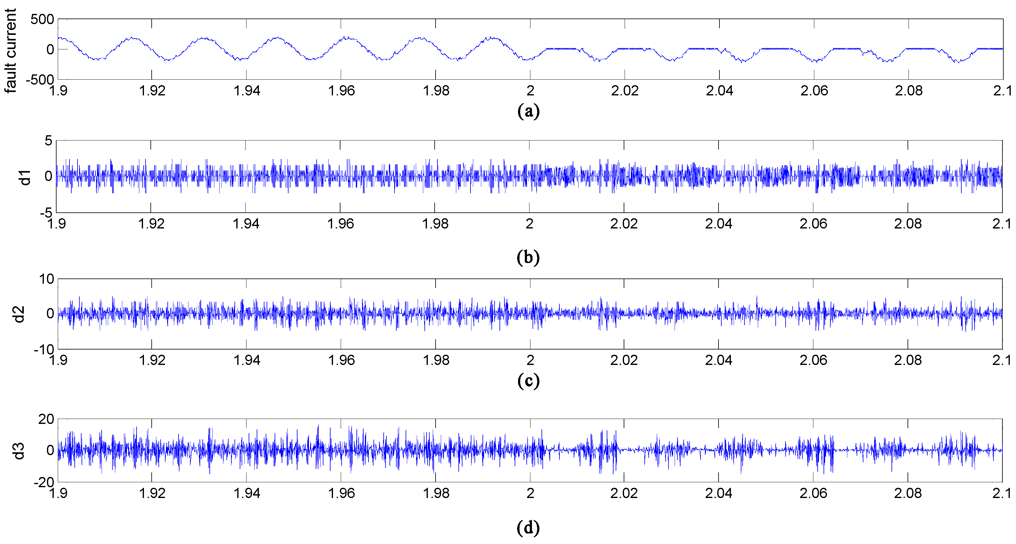
Utilize the FFT to determine the extra components of the normal current and fault current. By analyzing the frequency of each sub-band of DWPT, the sub-band that do not contain the extra component is selected. In this case, the sixth node in the third level is selected.
(2)
The parameters such as the length of the sliding window L and the sliding factor a should be set.
(3)
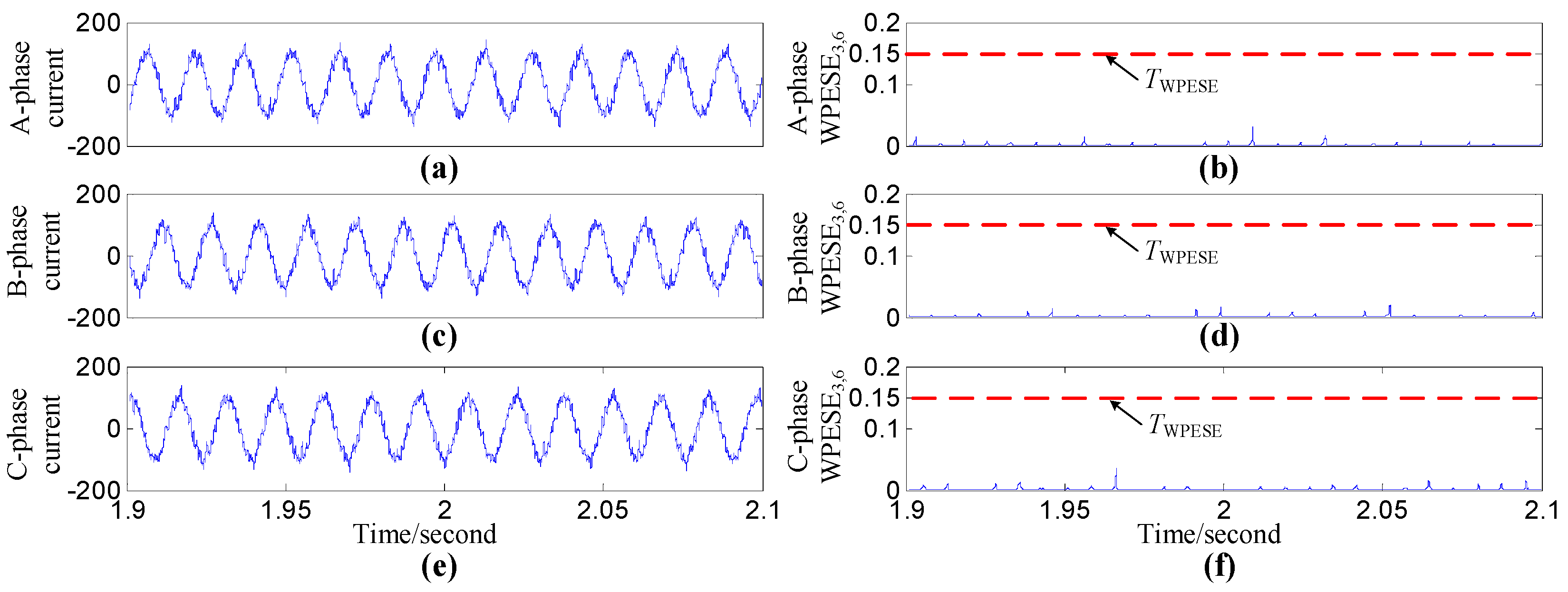
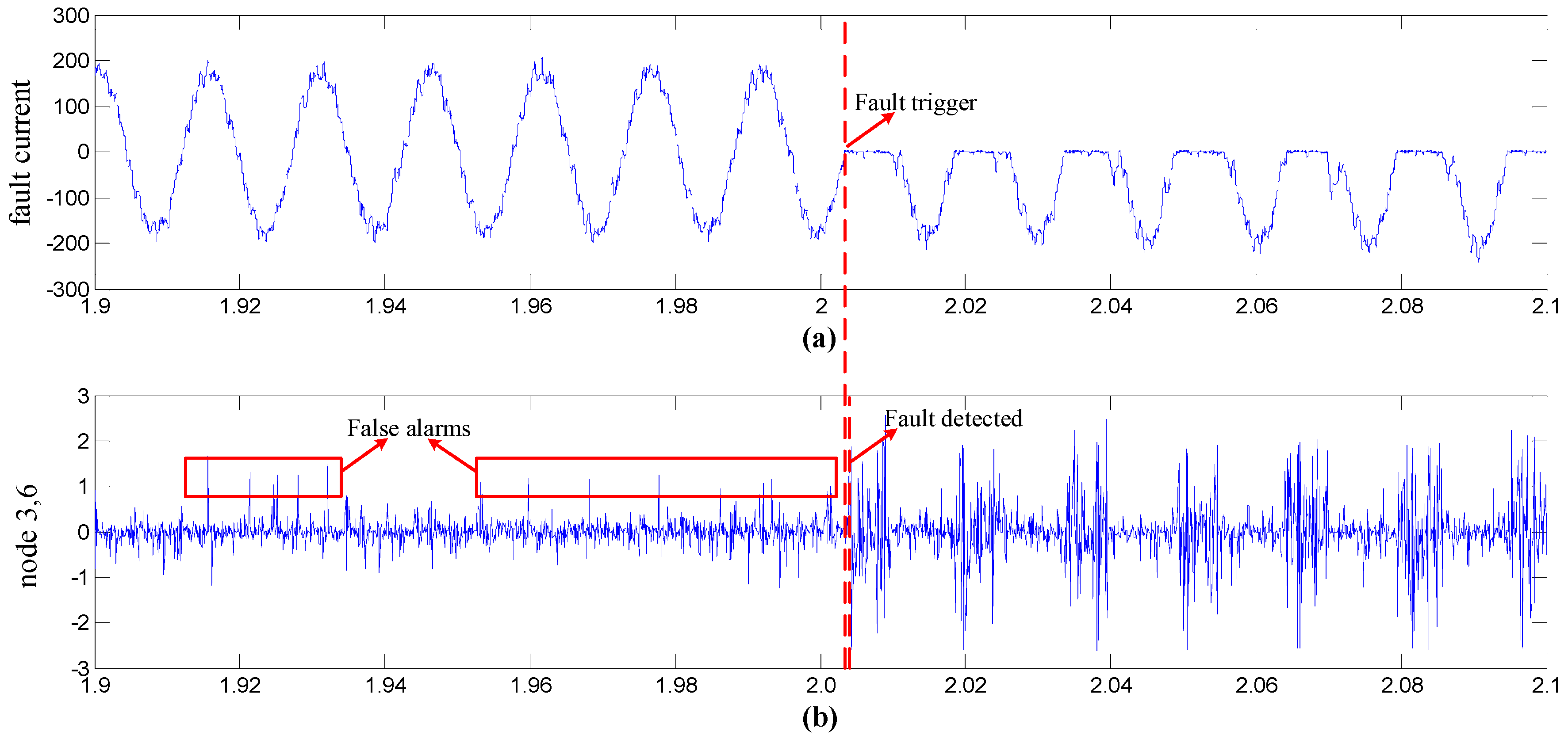
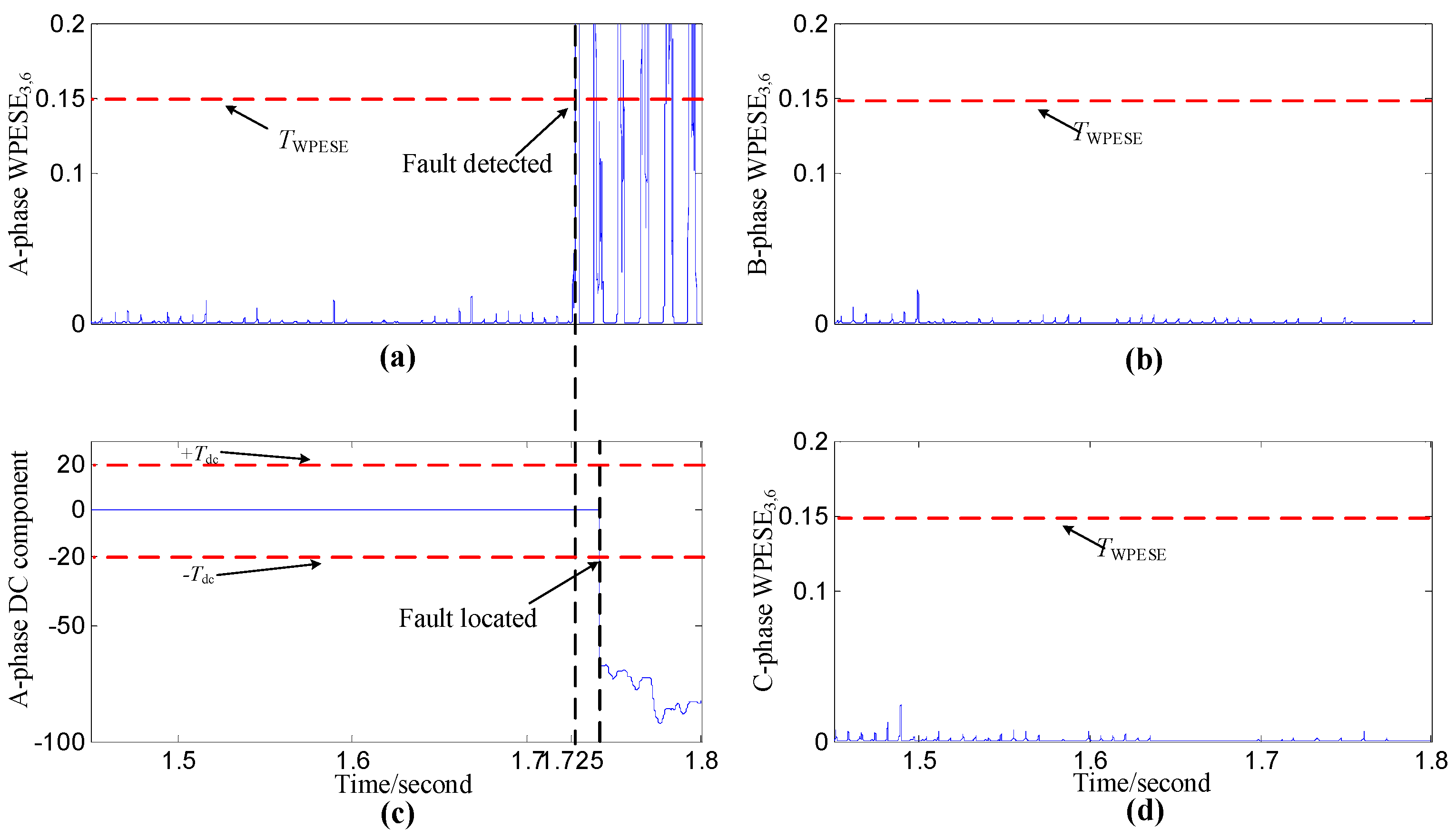
The WPESE3,6 of each phase current in the sliding window should be calculated. If the WPESE3,6 exceeds the predefined threshold TWPEE, the corresponding leg is faulty.
(4)
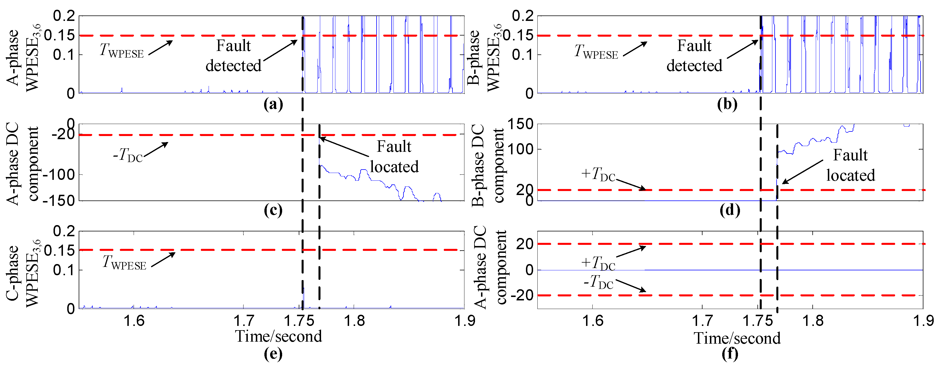
If a leg is detected as faulty, DC component Idc of the corresponding phase current in the next cycle shold be calculated. If Idc is larger than +TDC, the LSF is isolated. If Idc is less than −TDC, the LSF is isolated. Otherwise, simultaneous USF and LSF are isolated.

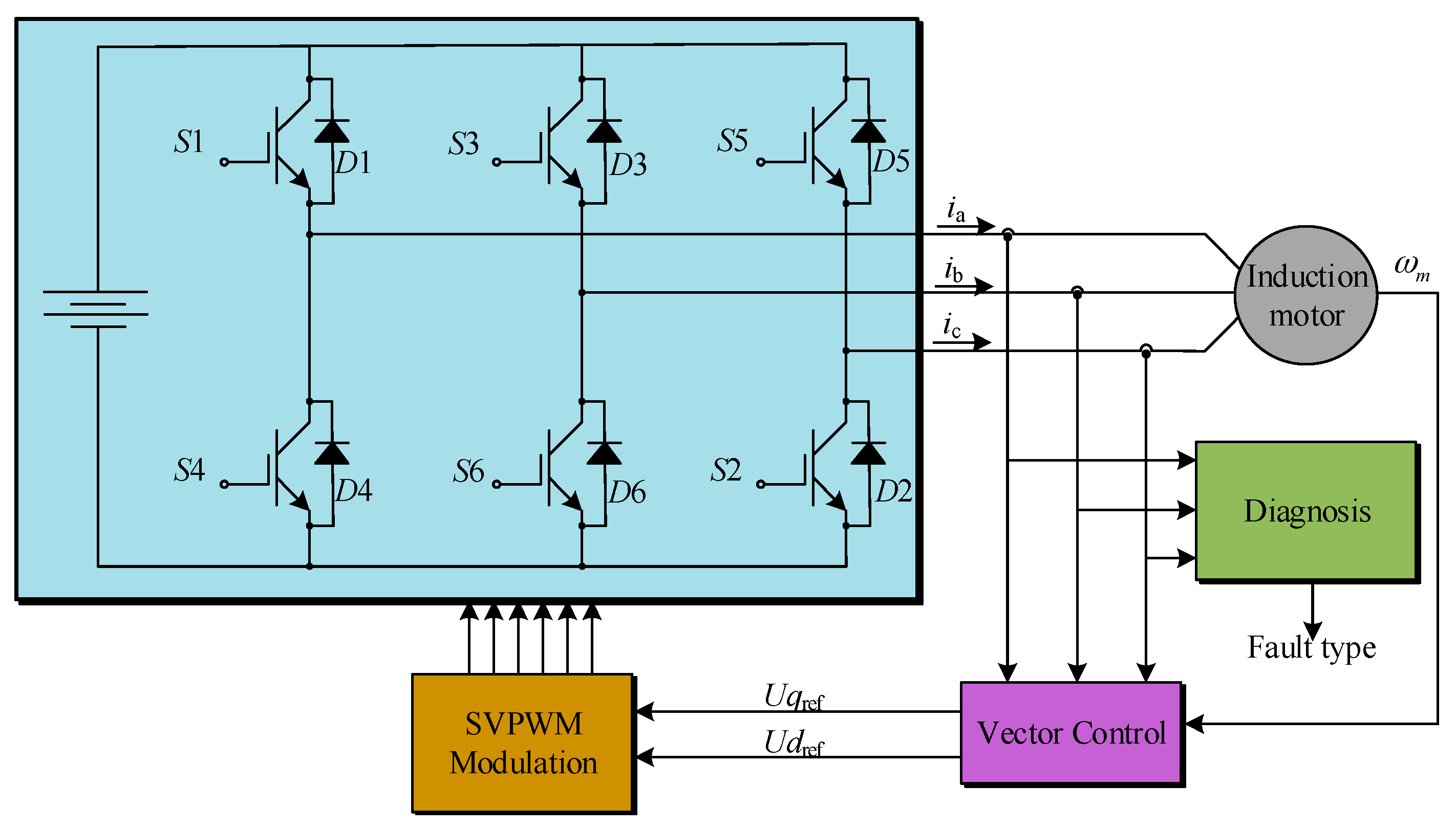
4. Simulation and Discussion
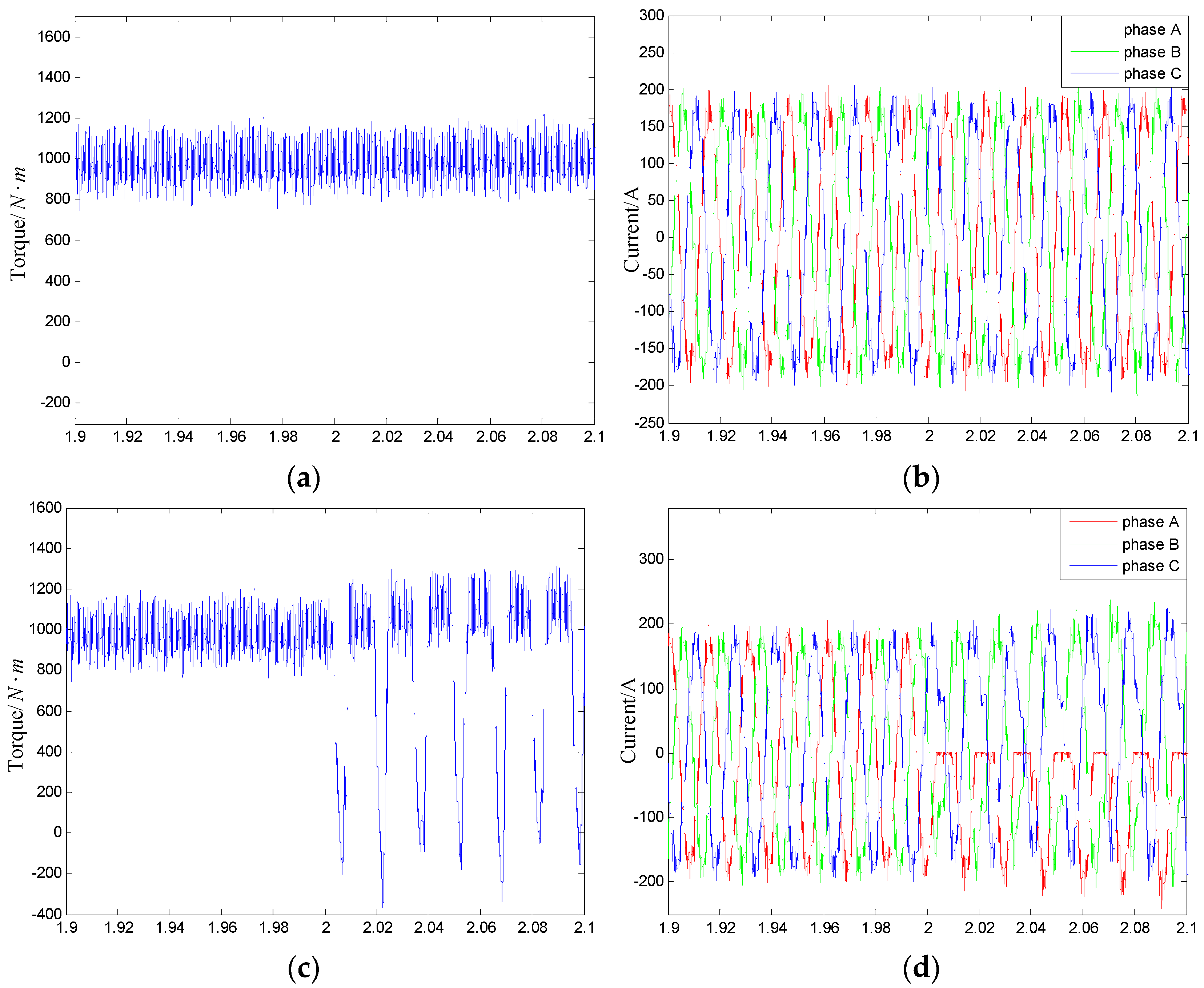
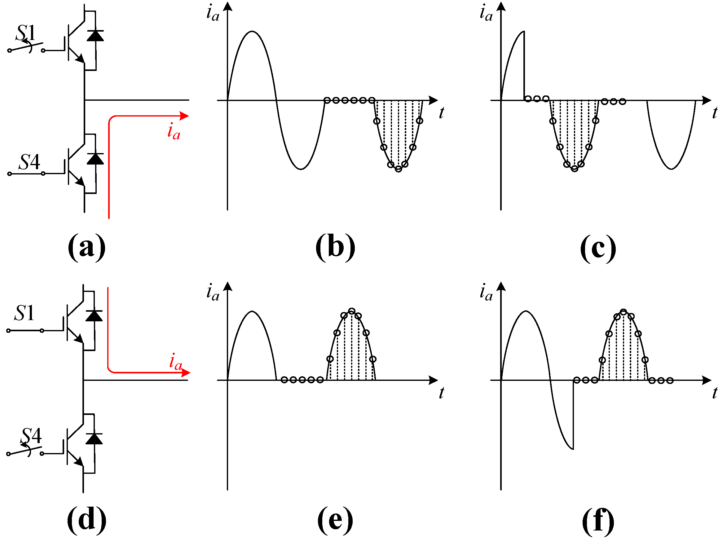
To validate the effectiveness of the idea proposed in this paper, simulation evaluation is carried out. A closed loop controlled traction system simulation model is established in SIMULINK. This system mainly comprises a traction motor (a squirrel cage induction motor), a traction inverter and a control part, as shown in Figure 1. The control part takes the responsibility for performing vector control and diagnosis. Space vector pulse width modulation is adopted to drive the traction inverter. The open switch fault is carried out by removing the drive signal of the corresponding IGBT and the anti-paralleled diode can still work. Forward voltage of each IGBT and paralelled diode is 1.4 V, fall time and tail of time each IGBT are 1 μs and 2 μs, respectively. The parameters of the traction motor are shown in Table 3.
The voltage of the DC bus is 3000 V and the switch frequency is 12.5 kHz. In this section, two kinds of traction inverter open switch faults are considered:
Fault A:
Just one open switch fault occurs at leg A on the upper IGBT(S1).
Fault B:
Two simultaneous open switch faults occur at leg A on the upper IGBT(S1) and at leg B on the lower IGBT(S6).

4.1. Fault-Free Case
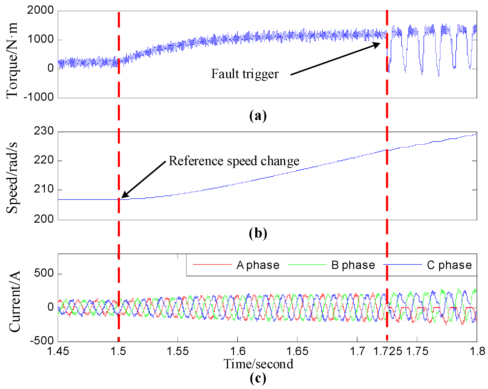
In order to prove that the proposed method will not cause false alarms, the fault free condition is simulated. Because the WPESE3,6 is not zero in the normal condition, the threshold TWPESE must be set to distinguish between the normal condition and fault condition. If WPESE3,6 exceeds the TWPESE, it can be judged that the corresponding leg is faulty. According to experience, the threshold TWPESE is set to 0.15, +TDC and −TDC are set to 20 and −20 respectively, the length of sliding window is set to 50 sampling points and the sliding factor is selected as 1. Figure 17 depicts the current and WPESE3,6 in normal condition. It is clear that all the WPESE3,6 has not exceeded the threshold, showing the proposed method will not cause false alarm in normal condition.

4.2. Fault A Case

To validate the effectiveness of the proposed plan in single fault condition, the S1 fault (fault A) is set at 1.725 s. The reference speed change is set as well to show that the proposed plan is robust to speed changes and torque changes.
As depicted in Figure 18, the reference speed is changed from 208 rad/s to 500 rad/s at 1.5 s and the torque is changed correspondingly. The open switch fault occurs on S1 at 1.725 s. Figure 19 shows the WPESE3,6 of each phase and the DC component of A phase. It can be seen that when the speed and torque change, the phase current becomes larger. However, the WPESE3,6 of each phase maintains unchanged, which means the WPESE3,6 is insensitive to the speed change and torque change. When the fault occurs, the WPESE3,6 of A phase exceeds the TWPEE while B phase’s and C phase’s do not, indicating that only A phase leg is faulty. After the A leg is detected as faulty, the DC component of A phase should be calculated. As Figure 19c shows, the A-phase DC component has exceeded the −TDC, the S1 open switch fault is diagnosed, and the diagnosis time is about one cycle.

4.3. Fault B Case

To validate the performance of the proposed diagnosis plan under simultaneous faults condition, S1 fault and S6 fault (fault B) are set at 1.75 s, and the reference speed change is set as well in this condition. Figure 20 depicts WPESE3,6 and DC component of each phase. A-phase WPESE3,6 and B-phase WPESE3,6 has exceeded the threshold at 1.755 s, indicating that there are faults at leg A and leg B.
Though there is a smallish C phase WPESE3,6 pulse at 1.755 s, it does not exceed the threshold, so no false alarm is caused. By calculating the DC component of each fault phase, USF of A leg and LSF of B leg are identified, i.e., S1 and S6 open switch faults are diagnosed, and the diagnosis time is about one cycle. Simulation validation of the proposed plan is implemented in this section. The results show that the proposed plan is robust to speed and torque changes, i.e., when the speed and torque of the traction motor change, no false alarms will be caused. In addition, the WPESE3,6 of each phase is independent of other phases, which makes faulty leg detection possible. The DC component can isolate the failure IGBT. Both single fault and simultaneous faults can be diagnosed in about one cycle.

5. Conclusions

Aiming at the problem of open switch faults of traction inverters in high-speed railways, a diagnosis plan is proposed in this paper. This plan contains two steps, namely, the fault detection part with entropy approach and fault location part with DC component approach. In the fault detection part, traditional fault detection methods, namely, DWT and DWPT, are discussed at first. Both of them cannot efficiently detect the open switch faults of traction inverters because of low resolution or the sudden change of the current. Then, the performances of five entropy forms, including WPESE, WPETE, WPESE3,6 EMDESE, EMDETE, were discussed for the open switch fault detection, and the evaluation parameter γ is defined to evaluate them. The comparison results show that the system is non-extensive and non-extensive parameter q = 0.9 for WPETE and q = 0.5 for EMDETE are most suitable, respectively. Tsallis entropies of DWPT and EMD have better detection performance than their Shannon entropies for the open switch fault detection. However, WPESE3,6 gets rid of the extra components by selecting the sixth node of the third level of DWPT, and the effects of the currents’ sudden change is eliminated. Hence the WPESE3,6 has the best performance.
In the fault location part, DC component is adopted to settle the problem that entropy is not directional as it is calculated by absolute value. DC component will exceed the positive threshold for LSF and exceed the negative threshold for USF. In addition, the single fault and simultaneous faults simulation experiments are implemented, and the results show that the proposed diagnosis plan can identify the failure IGBT in about one cycle correctly.

Acknowledgments

This study is partly supported by National Nature Science Foundation of China (No. U1434203, 51377136) and Sichuan Province Youth Science and Technology Innovation Team (No. 2016TD0012).

Author Contributions

The individual contribution of each co-author to the reported research and writing of the paper are as follows. Zhigang Liu and Keting Hu conceived the idea, Keting Hu and Shuangshuang Lin performed experiments and data analysis, and all authors wrote the paper. All authors have read and approved the final manuscript.

Conflicts of Interest

The authors declare no conflict of interest.

Nomenclature

DWPTDiscrete Wavelet Packet Transform
DWTDiscrete Wavelet Transform
EMDEmpirical Mode Decomposition
EMDESEEmpirical Mode Decomposition Shannon Entropy
EMDETEEmpirical Mode Decomposition Tsallis Entropy
IGBTIsolated Gate Bipolar Transistor
LSFLower Switch Fault
SPDSemiconductor Power Devices
TDCThreshold for the DC component
TWESEThreshold for the WPESE3,6
USFUpper Switch Fault
WPETEWavelet Packet Energy Tsallis Entropy
WPESEWavelet Packet Energy Shannon Entropy
γ 
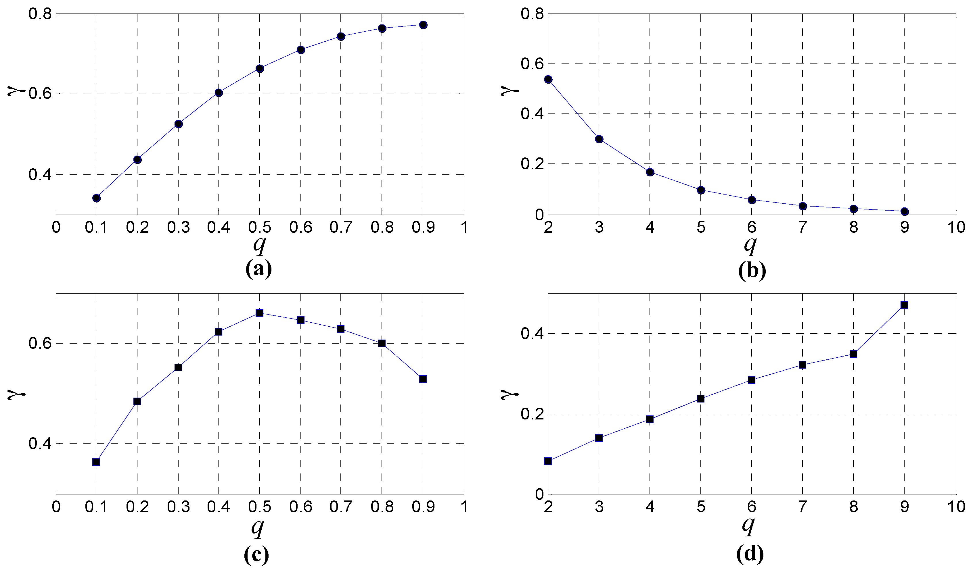
Evaluation parameter for different entropies

References

  1. Smet, V.; Forest, F.; Huselstein, J.-J.; Richardeau, F.; Khatir, Z.; Lefebvre, S.; Berkani, M. Ageing and failure modes of IGBT modules in high-temperature power cycling. IEEE Trans. Ind. Electron. 2011, 58, 4931–4941. [Google Scholar] [CrossRef]
  2. Campos-Delgado, D.U.; Espinoza-Trejo, D.R.; Palacios, E. Fault-tolerant control in variable speed drives: A survey. IET Electr. Power Appl. 2008, 2, 121–134. [Google Scholar] [CrossRef]
  3. Mirafzal, B. Survey of Fault-Tolerance Techniques for Three-Phase Voltage Source Inverters. IEEE Trans. Ind. Electron. 2014, 61, 5192–5202. [Google Scholar] [CrossRef]
  4. Yang, S.; Bryant, A.; Mawby, P.; Xiang, D.; Ran, L.; Tavner, P. An industry-based survey of reliability in power electronic converters. IEEE Trans. Ind. Appl. 2011, 47, 1441–1451. [Google Scholar] [CrossRef]
  5. Lu, B.; Sharma, S.K. A literature review of IGBT fault diagnostic and protection methods for power inverters. IEEE Trans. Ind. Appl. 2009, 45, 1770–1777. [Google Scholar]
  6. An, Q.T.; Sun, L.Z.; Zhao, K.; Sun, L. Switching function model-based fast-diagnostic method of open-switch faults in inverters without sensors. IEEE Trans. Power Electron. 2011, 26, 119–126. [Google Scholar] [CrossRef]
  7. Campos-Delgado, D.U.; Espinoza-Trejo, D.R. An observer-based diagnosis scheme for single and simultaneous open-switch faults in induction motor drives. IEEE Trans. Ind. Electron. 2011, 58, 671–679. [Google Scholar] [CrossRef]
  8. Freire, N.M.; Estima, J.O.; Cardoso, A.J.M. A voltage-based approach without extra hardware for open-circuit fault diagnosis in closed-loop PWM AC regenerative drives. IEEE Trans. Ind. Electron. 2014, 61, 4960–4970. [Google Scholar] [CrossRef]
  9. Salehifar, M.; Salehi Arashloo, R.; Moreno-Eguilaz, M.; Sala, V.; Romeral, L. Observer-based open transistor fault diagnosis and fault-tolerant control of five-phase permanent magnet motor drive for application in electric vehicles. IET Power Electron. 2014, 8, 76–87. [Google Scholar] [CrossRef]
  10. Estima, J.O.; Marques Cardoso, A.J. A new algorithm for real-time multiple open-circuit fault diagnosis in voltage-fed PWM motor drives by the reference current errors. IEEE Trans. Ind. Electron. 2013, 60, 3496–3505. [Google Scholar] [CrossRef]
  11. Estima, J.O.; Cardoso, A.J.M. A new approach for real-time multiple open-circuit fault diagnosis in voltage-source inverters. IEEE Trans. Ind. Appl. 2011, 47, 2487–2494. [Google Scholar] [CrossRef]
  12. Choi, U.M.; Jeong, H.G.; Lee, K.B.; Blaabjerg, F. Method for detecting an open-switch fault in a grid-connected NPC inverter system. IEEE Trans. Power Electron. 2012, 27, 2726–2739. [Google Scholar] [CrossRef]
  13. Choi, J.-H.; Kim, S.; Yoo, D.S.; Kim, K.-H. A Diagnostic Method of Simultaneous Open-Switch Faults in Inverter-fed Linear Induction Motor Drive for Reliability Enhancement. IEEE Trans. Ind. Electron. 2014, 62, 4065–4077. [Google Scholar] [CrossRef]
  14. Khanniche, M.S.; Mamat-Ibrahim, M.R. Wavelet-fuzzy-based algorithm for condition monitoring of voltage source inverter. Electron. Lett. 2004, 40, 267–268. [Google Scholar] [CrossRef]
  15. Keswani, R.A.; Suryawanshi, H.M.; Ballal, M.S. Multi-resolution analysis for converter switch faults identification. IET Power Electron. 2015, 8, 783–792. [Google Scholar] [CrossRef]
  16. Aktas, M.; Turkmenoglu, V. Wavelet-based switching faults detection in direct torque control induction motor drives. IET Sci. Meas. Technol. 2010, 4, 303–310. [Google Scholar] [CrossRef]
  17. Dong, E.K.; Dong, C.L. Fault diagnosis of three-phase PWM inverters using wavelet and SVM. J. Power Electron. 2009, 9, 377–385. [Google Scholar]
  18. Cui, J. Faults Classification of Power Electronic Circuits Based on a Support Vector Data Description Method. Metrol. Meas. Syst. 2015, 22, 205–220. [Google Scholar] [CrossRef]
  19. Hu, Z.K.; Gui, W.H.; Yang, C.H.; Deng, P.C.; Ding, S.X. Fault classification method for inverter based on hybrid support vector machines and wavelet analysis. Int. J. Control Autom. Syst. 2011, 9, 797–804. [Google Scholar] [CrossRef]
  20. Liu, Z.G.; Han, Z.W.; Zhang, Y. Multiwavelet packet entropy and its application in transmission line fault recognition and classification. IEEE Trans. Neural Netw. Learn. Syst. 2014, 25, 2043–2052. [Google Scholar] [CrossRef] [PubMed]
  21. Liu, Z.G.; Cui, Y.; Li, W.H. Complex power quality disturbances recognition using wavelet packet entropies and S-transform. Entropy 2015, 17, 5811–5828. [Google Scholar] [CrossRef]
  22. Dubey, R.; Samantaray, S.R. Wavelet singular entropy-based symmetrical fault-detection and out-of-step protection during power swing. IET Gener. Transm. Distrib. 2013, 7, 1123–1134. [Google Scholar] [CrossRef]
  23. Yang, Q.; Wang, J. Multi-Level Wavelet Shannon Entropy-Based Method for Single-Sensor Fault Location. Entropy 2015, 17, 7101–7117. [Google Scholar] [CrossRef]
  24. Lei, Y.; He, Z.; Zi, Y. Application of the EEMD method to rotor fault diagnosis of rotating machinery. Mech. Syst. Signal Process. 2009, 23, 1327–1338. [Google Scholar] [CrossRef]
  25. Lei, Y.; Lin, J.; He, Z.; Zuo, M. A review on empirical mode decomposition in fault diagnosis of rotating machinery. Mech. Syst. Signal Process. 2013, 35, 108–126. [Google Scholar] [CrossRef]
  26. Yu, Y.; Junsheng, C. A roller bearing fault diagnosis method based on EMD energy entropy and ANN. J. Sound Vib. 2006, 294, 269–277. [Google Scholar] [CrossRef]
Figure 1. Schematic diagram of the vector controlled traction system.
Entropy 18 00078 g001
Figure 2. (a) A-phase torque in normal state; (b) A-phase currents in normal state; (c) A-phase torque when S1 open switch fault occurs; (d) A-phase currents when S1 open switch fault occurs.
Entropy 18 00078 g002
Figure 3. Wavelet decomposition.
Entropy 18 00078 g003
Figure 4. (a) A-phase fault current with S1 open (50 kHz sampling frequency); (b) First level detail coefficient; (c) Second level detail coefficient; (d) Third level detail coefficient.
Entropy 18 00078 g004
Figure 5. (a) spectrum of fault free current (50 kHz sampling frequency and 0.2 s acquisition time); (b) spectrum of A-phase fault current with S1 open (50 kHz sampling frequency and 0.2 s acquisition time).
Entropy 18 00078 g005
Figure 6. Frequency of each sub-band after wavelet packet decomposition.
Entropy 18 00078 g006
Figure 7. (a) A-phase fault current with S1 open; (b) Coefficients of the sixth node in the third level.
Entropy 18 00078 g007
Figure 8. (a) WPESE of A-phase fault current with S1 open; (b) WPETE of A-phase fault current with S1 open when q = 0.1; (c) WPETE of A-phase fault current with S1 open when q = 0.5; (d) WPETE of A-phase fault current with S1 open when q = 0.9.
Entropy 18 00078 g008
Figure 9. (a) WPESE of A-phase fault current with S1 open; (b) WPETE of A-phase fault current with S1 open when q = 2; (c) WPETE of A-phase fault current with S1 open when q = 5; (d) WPETE of A-phase fault current with S1 open when q = 9.
Entropy 18 00078 g009
Figure 10. WPETE3,6 of fault current.
Entropy 18 00078 g010
Figure 11. EMD results of A-phase fault current with S1 open.
Entropy 18 00078 g011
Figure 12. (a) EMDESE of A-phase fault current with S1 open; (b) EMDETE of A-phase fault current with S1 open when q = 0.1; (c) EMDETE of A-phase fault current with S1 open when q = 0.5; (d) EMDETE of A-phase fault current with S1 open when q = 0.9.
Entropy 18 00078 g012
Figure 13. (a) EMDESE of A-phase fault current with S1 open; (b) EMDETE of A-phase fault current with S1 open when q = 2; (c) EMDETE of A-phase fault current with S1 open when q = 5; (d) EMDETE of A-phase fault current with S1 open when q = 9.
Entropy 18 00078 g013
Figure 14. (a) WPETE of fault current when q is in the range of [0.1,0.9]; (b) WPETE of fault current when q is in the range of [2,9]; (c) EMDETE of fault current when q is in the range of [0.1,0.9]; (d) EMDETE of fault current when q is in the range of [2,9].
Entropy 18 00078 g014
Figure 15. (a) Current flow of USF; Current wave when USF occurs in(b) negative current flow; (c) positive current flow; (d) Current flow of LSF; Current wave when LSF occurs in (e) positive current flow; (f) negative current flow.
Entropy 18 00078 g015
Figure 16. Flow chart of the proposed method.
Entropy 18 00078 g016
Figure 17. (a) A-phase current in normal condition; (b) A-phase WPESE3,6; (c) B-phase current in normal condition; (d) B-phase WPESE3,6; (e) C-phase current in normal condition; (f) C-phase WPESE3,6.
Entropy 18 00078 g017
Figure 18. Normal condition (a) Torque; (b) Speed of the traction motor; (c) Three phase current.
Entropy 18 00078 g018
Figure 19. Fault A condition (a) A-phase WPESE3,6; (b) B-phase WPESE3,6; (c) A-phase DC component; (d) C-phase WPESE3,6.
Entropy 18 00078 g019
Figure 20. Fault B condition (a) A-phase WPESE3,6; (b) B-phase WPESE3,6; (c) A-phase DC component; (d) B-phase DC component; (d) C-phase WPESE3,6; (f) C-phase DC component.
Entropy 18 00078 g020
Table 1. Frequency range of each sub-band.
Sub-BandFrequency Range
D1[525,1050] Hz
D2[262.5,525] Hz
D3[131.25,262.5] Hz
Table 2. Evaluation parameter of each entropy form.
Entropy FormEvaluation Parameter γ
WPESE0.21
WPETE0.90.7724
WPESE3,63.124
EMDESE0.498
EMDETE0.50.66
Table 3. Parameters of the traction motor.
ParameterValue
Stator resistance/Rs0.15 Ω
Stator inductance/Ls0.00142 H
Rotator resistance/Rr0.16 Ω
Rotator inductance/Lr0.006 H
Mutual inductance/Lm0.0254 H
Inertia/J10 kg·m2
Nominal line voltage2700 V
Nominal frequency138 Hz
Pole pairs2
Nominal power562 kVA

