Monitoring Test for Stability of Dependence Structure in Multivariate Data Based on Copula

Abstract

In this paper, we consider a sequential monitoring procedure for detecting changes in copula function. We propose a cusum type of monitoring test based on the empirical copula function and apply it to the detection of the distributional changes in copula function. We investigate the asymptotic properties of the stopping time and show that under regularity conditions, its limiting null distribution is the same as the sup of Kiefer process. Moreover, we utilize the bootstrap method in order to obtain the limiting distribution. A simulation study and a real data analysis are conducted to evaluate our test.

1. Introduction

A copula is a multivariate joint distribution function for which the marginal distribution of each variable is uniform. In classical analysis, the Pearson’s correlation is most frequently used in practice as a measure of dependence. However, it only works well with elliptical distributions while empirical data in finance and insurance mostly has skewed distributions, heavy tails and extreme values. Thus, correlation may not be suitable to model the nonlinear association. The copula function can overcome this drawback due to the fact that a copula can model various types of dependence structure beyond the linear dependence independently of the marginal distributions. For this reason, a copula has become a flexible methodology in applications of financial risk assessment and actuarial analysis (see Cherubini et al. [1,2], McNeil et al. [3], Hougaard [4] and the papers cited therein). Recently, dependence modelling with copula function has been widely applied to various areas such as civil engineering, reliability engineering, climatology, hydrology, biology, etc.

Since all of the information about the dependence is contained in the copula function, estimating the copula function is a crucial task for providing a correct dependence structure. Conventionally, the copula function is assumed to remain constant over time. However, there is empirical evidence suggesting that the dependence structure is likely to change due to some financial adjustments and critical social events (see, for example, Longin and Solnik [5], Patton [6] and Rodriguez [7]). To cope with this, Dias and Embrechts [8] and Guegan and Zhang [9] suggested a likelihood ratio test for copula parameter changes in specific copula families, Harvey [10] and Busetti and Harvey [11] developed a nonparametric stationarity test for a constant copula based on time-varying quantiles, and Na et al. [12] studied a cusum test for detecting the copula parameter change.

Recently, the problem of testing constancy of the copula has been studied by Quessy et al. [13], Bücher and Ruppert [14], and Bücher et al. [15]. All of these approaches are devoted to the change point detection within data sets of fixed size. However, many researchers are also interested in monitoring change over time when new observations are sequentially observed. Chu et al. [16] pointed out that repeated application of the retrospective tests each time new data is observed may result in a high probability of type I error as the number of applications grows. In this study, we focus on the monitoring procedure for the early detection of a copula function change. During the past few decades, the monitoring procedure has been studied by many authors. For instance, Chu et al. [16] and Horváth et al. [17] developed a cusum type monitoring procedure for detecting structural changes in linear regression models. Berkes et al. [18] applied the monitoring test to generalized autoregressive conditional heteroscedastic (GARCH) models based on quasi-likelihood score. Gombay and Serban [19] monitored parameter changes in autoregressive (AR) models using the cusum type method. Na et al. [20] designed the monitoring test in general time series models.

Recently, Na et al. [21] developed a monitoring procedure to detect a change of the copula parameter. However, one major drawback of this test is that the test statistic is derived under the assumption that the copula family does not change. In this regard, we attempt to develop a monitoring procedure that is more general than their test against alternatives that involve a change in copula function. For this task, we extend the approach of Lee et al. [22] who sequentially monitored distributional changes in AR models and proposed the test statistic based on the empirical copula function. It is shown that, under regularity conditions, the stopping time designed for the detection of changes behaves asymptotically the same as the Kiefer process. In practice, however, the Kiefer process depends on the unknown copula and is rather complicated to compute. To overcome this problem, several authors have suggested bootstrap methods for approximating the Kiefer process. We refer to Fermanian et al. [23], Rémillard and Scaillet [24], Bücher and Dette [25], Bouzebda [26] and the references therein for more details. In this study, we also utilize the bootstrap method to deal with this difficulty.

This paper is organized as follows. We introduce the monitoring procedure based on the empirical copula process in Section 2 and establish some asymptotic results of the stopping time in Section 3. In Section 4, we report some simulation results that validate our monitoring procedure, and apply the test to real data analysis. In Section 5, conclusions with a brief discussion of the advantages and limitations of our study are provided.

2. Monitoring Procedure

Let $\{{\mathbb{X}}_t=(X_{1t},\cdots ,X_{dt});t=1,2,\cdots \}$ be a sequence of d-dimensional independent random vectors with joint distribution F and continuous marginal distribution functions $F_i$ for $i=1,\cdots ,d$. If C is a true copula function of $\{{\mathbb{X}}_t\}$, owing to Sklar’s theorem, we can express

$$\begin{array}{c}\hfill F(x_1,\cdots ,x_d)=C(F_1(x_1),\cdots ,F_d(x_d))\mathrm{for}(x_1,\cdots ,x_d)\in {\mathbb{R}}^d.\end{array}$$

When the marginal distribution functions $F_1,\cdots ,F_d$ are continuous, it is well known that the function C is uniquely determined such as

$$\begin{array}{c}\hfill C(u_1,\cdots ,u_d)=F(F_1^{-}(u_1),\cdots ,F_d^{-}(u_d))\mathrm{for}(u_1,\cdots ,u_d)\in {[0,1]}^d,\end{array}$$

(1)

where $F_i^{-}(u_i)=inf\{x:F_i(x)\ge u_i\}$ for $i=1,\cdots ,d$. According to Sklar’s theorem, one can always model any multivariate distributions by modelling both marginal distributions and copula functions separately. For details, we refer to Joe [27] and Nelson [28].

Suppose that we have observed ${\mathbb{X}}_1,\dots ,{\mathbb{X}}_n$, which are called the historical data. For each new observation, we wish to test the following hypotheses:

$$H_0:C_t=C\text{ for all }t>n,\text{ vs}.H_1:C_t\ne C\text{ for some }t>n,$$

where $C_t$ is a copula function at time t and C is a time-invariant copula. The copula function is assumed to be stable over the historical period of length n, i.e.,

$$C_t=C,1\le t\le n.$$

The historical data is used as a reference for comparison with future observations. The aim of our monitoring procedure is to check a change of copula function each time a new observation is updated in the post-historical period.

In this study, we assume that the marginal distributions do not change under both the null and alternative hypotheses, while the copula function changes under the alternative hypothesis. This assumption is in line with other precedent studies on testing for structural breaks in copula (see, e.g., Harvey [10], Busetti and Harvey [11], Bouzebda [26], Bücher and Ruppert [14] and Na et al. [12,21]). Furthermore, this assumption is very crucial in real practice since one can encounter the situation that the monitoring test detects a change in copula function although the change actually occurs in marginal distributions. Empirical evidence of this situation can be found in Na et al. [29]. Therefore, a change point test for marginal distribution must be conducted in advance of implementing the monitoring test for a copula function change.

The monitoring procedure in a general set-up can be described with the stopping time $\tau (n)$ defined as follows:

$$\begin{array}{c}\hfill \tau (n):=inf\{k>n:D_{k,n}\ge b(k/n)\},\end{array}$$

(2)

where $D_{k,n}$ is a test statistic based on ${\mathbb{X}}_1,\dots ,{\mathbb{X}}_k$ and $b(·)$ is a boundary function. If $\tau (n)$ is finite, we reject $H_0$ and consider that the change has occurred at $\tau (n)$. Otherwise, we continue to observe the data. Therefore, in order to perform the monitoring procedure, we have to define a test statistic $D_{k,n}$ and choose a boundary function $b(·)$ such that

$$\begin{array}{c}\hfill \underset{n\to \infty }{lim}P\{\tau (n)<\infty |H_0\}=\underset{n\to \infty }{lim}P\{D_{k,n}\ge b(k/n)\mathrm{for}\mathrm{some}k>n|H_0\}=\alpha \end{array}$$

(3)

for a given $\alpha \in (0,1)$, and

$$\begin{array}{c}\hfill \underset{n\to \infty }{lim}P\{\tau (n)<\infty |H_1\}=1.\end{array}$$

We consider the boundary function $b(·)$ satisfies:

$$\begin{array}{c}\hfill b(s)\text{is continuous on}(1,\infty )\mathrm{and}\underset{1<s<\infty }{inf}b(s)>0\end{array}$$

(4)

(cf. Chu et al. [16] and Berkes at al. [18]). Here, we focus on the $b(·)$ of a specific form such as

$$\begin{array}{c}\hfill b(s)=c{s}^a\mathrm{for}\mathrm{some}c>0,a>0,\end{array}$$

(5)

proposed by Lee et al. [22]. Practically, the constants c and a must be chosen to satisfy (3) for a given α.

For the specific form of test statistic $D_{k,n}$, Chu et al. [16] considered two types of test statistics. The one is based on the fluctuations of sequential parameter estimates, and the other is based on the cumulative sum of recursive residuals. Berkes [18] proposed the quasi–maximum likelihood estimator of the parameters in the GARCH process for test statistics. Lee et al. [22] used a sequential empirical process of residuals for the detection of distributional changes in AR models.

In this paper, we use a copula function for the test statistic to detect a change in the dependence structure of multivariate random vectors. The main idea of the procedure is based on the changes in the dependence structure upon changes in the copula function. In real practice, the copula function C is usually unknown. Thus, we consider the situation in which the empirical copula estimator is employed to play a role of the true copula function. The empirical copula function can be obtained by replacing the unknown terms in (1) with the joint empirical distribution function and the marginal empirical distribution function, which are defined, respectively, by

$$\begin{array}{c}\hfill F_n(x_1,\cdots ,x_d)=\frac{1}{n}\sum _{t=1}^{n}I(X_{1t}\le x_1,\cdots ,X_{dt}\le x_d)\mathrm{for}{x}_i\in \mathbb{R},\end{array}$$

$$\begin{array}{c}\hfill F_{in}(x_i)=\frac{1}{n}\sum _{t=1}^{n}I(X_{it}\le x_i)\mathrm{for}i=1,\cdots ,d.\end{array}$$

Then, the empirical copula estimator is

$$\begin{array}{c}\hfill C_{n,n}(u_1,\cdots ,u_d)={\mathrm{F}}_n(F_{1n}^{-}(u_1),\cdots ,F_{dn}^{-}(u_d))\mathrm{for}{u}_i\in [0,1],\end{array}$$

(6)

where $F_{in}^{-}(u_i)=inf\{x:F_{in}(x)\ge u_i\}$ for $i=1,\cdots ,d$. Set $U_{it}=F_i(X_{it})$, for $i=1,\cdots d$. Then, for $u_i\in [0,1]$, $G_n$ and $G_{in}$ can be expressed as

$$\begin{array}{c}\hfill G_n(u_1,\cdots ,u_d)=\frac{1}{n}\sum _{t=1}^{n}I(U_{1t}\le u_1,\cdots ,U_{dt}\le u_d)\end{array}$$

and

$$\begin{array}{c}\hfill G_{in}(u_i)=\frac{1}{n}\sum _{t=1}^{n}I(U_{it}\le u_i)\mathrm{for}i=1,\cdots ,d.\end{array}$$

Then, we have

$$\begin{array}{c}\hfill F_n(x_1,\cdots ,x_d)\stackrel{d}{=}{G}_n(F_1(x_1),\cdots ,F_d(x_d))\end{array}$$

and

$$\begin{array}{c}\hfill (F_{1n}(x_1),\cdots ,F_{dn}(x_d))\stackrel{d}{=}(G_{1n}(F_1(x_1)),\cdots ,G_{dn}(F_1(x_d))).\end{array}$$

Thus, using the representation (6), it follows that

$$\begin{array}{c}\hfill C_{n,n}(u_1,\cdots ,u_d)\stackrel{d}{=}{G}_n(G_{1n}^{-}(u_1),\cdots ,G_{dn}^{-}(u_d)),\end{array}$$

where $G_{in}^{-}(u_i)=inf\{x:G_{in}(x)\ge u_i\}$ for $i=1,\cdots ,d.$ This implies that the law of $C_{n,n}$ is the same for all F whose associated copula is C. We will propose the test statistics based on the empirical copula estimator in the next section.

Remark 1.

Note that the alternative hypothesis $H_1$ actually means that $H_1$ : $C_t\ne C$ for some $n<t<T(n)$, where $T(n)$ is the predetermined maximal number. Since it is impossible to monitor at an unlimited time horizon and the test for too large t will be meaningless, the maximal number of observations $T(n)$ is considered. Here, $T(n)$ is considered as ${lim}_{n\to \infty }\frac{T(n)}{n}=q<\infty$ and ${lim}_{n\to \infty }\frac{T(n)}{n}=\infty$, and this result will be seen in our simulation study.

3. Main Result

For monitoring the copula function, we employ the test statistic $D_{n,k}$ based on the empirical copula functions such as

$$\begin{array}{c}\hfill D_{k,n}=\sqrt{n}\underset{\mathbf{u}\in {[0,1]}^d}{sup}\left|C_{k,n}(\mathbf{u})-C_{n,n}(\mathbf{u})\right|,\end{array}$$

(7)

where $\mathbf{u}=(u_1,\cdots ,u_d)$ and $C_{k,n}(\mathbf{u})={\mathrm{F}}_k(F_{1n}^{-}(u_1),\cdots ,F_{dn}^{-}(u_d))$. Suppose that ${\mathbb{X}}_1,\dots ,{\mathbb{X}}_n$ are observed which represent available historical data. By observing new data sequentially, we wish to detect if a change occurs in copula function C. This procedure compares the estimates of the copula function obtained based on a growing number of observations, with the estimate obtained based on the historical observations. Note that $C_{k,n}$ is the estimator of C based on the observation up to time k, while $C_{n,n}$ is the estimator obtained based on the historical data. As mentioned earlier, since we assume that the marginal distribution functions are stable, the marginal empirical distribution functions $F_{in}$ are used in $C_{k,n}$ instead of $F_{ik}$.

To show the asymptotic behavior of the test statistic, we need to introduce some Gaussian processes. The limiting process ${\mathbf{K}}_C(·)$ on ${[0,1]}^d\times [0,\infty )$ is a Gaussian process with

$$\begin{array}{c}\hfill E({\mathbf{K}}_C(\mathbf{u},n))=0\end{array}$$

and

$$\begin{array}{c}\hfill E({\mathbf{K}}_C(\mathbf{u},n){\mathbf{K}}_C(\mathbf{v},m))=(n\wedge m)\left(C(\mathbf{u}\wedge \mathbf{v})-C(\mathbf{u})C(\mathbf{v})\right),\end{array}$$

for $\mathbf{u},\mathbf{v}\in {[0,1]}^d$ and $n,m\ge 0$. The process ${\mathbf{K}}_C(·)$ on ${[0,1]}^d\times [0,\infty )$ is called the Kiefer process associated with the copula function C. For details on the Kiefer process, we refer to Adler [30] and Piterbarg [31].

Here, we impose the following conditions for the main theorem:

(A1)

C is twice continuously differentiable on ${(0,1)}^d$;

(A2)

The second-order partial derivatives of C exist and are continuous on ${[0,1]}^d$;

(A3)

$\underset{n\to \infty }{lim}\underset{k\ge n}{sup}\frac{1}{b(k/n)}\frac{{(logk)}^{3/2}}{n^{1/4d}}=0.$

Under the above assumptions, we have the following:

Theorem 1.

Suppose that $H_0$ is true and conditions (A1) and (A2) hold. In addition, a boundary function $b(·)$ satisfies (4), (5) and condition (A3). Then, the stopping time $\tau (n)$ with a test statistic $D_{k,n}$ in (7) satisfies

$$\begin{array}{c}\hfill \underset{n\to \infty }{lim}P\{\tau (n)<\infty |H_0\}=P\{\underset{\mathit{u}\in {[0,1]}^d}{sup}\left|{\mathit{K}}_C(\mathit{u},s)\right|\ge b\left(\frac{1}{1-s}\right)forsome0<s<1\},\end{array}$$

where ${\mathit{K}}_C(·)$ is a ($d+1$)-dimensional Kiefer process on ${[0,1]}^d\times [0,\infty )$ associated with the copula function $C(·)$.

Proof of Theorem 1.

For convenience, we set $\mathbf{u}=(u_1,\cdots ,u_d)$ and $\mathbf{v}=(v_1,\cdots ,v_d)$. Then, we can rewrite

$$\begin{array}{c}\hfill C_{k,n}(\mathbf{u})=G_k(G_{1n}^{-}(u_1),\cdots ,G_{dn}^{-}(u_d))=I_k(\mathbf{u})+I{I}_{n,k}(\mathbf{u})+II{I}_n(\mathbf{u}),\end{array}$$

(8)

where

$$\begin{array}{c}\hfill I_k(\mathbf{u})=G_k(\mathbf{u})-C(\mathbf{u}),\end{array}$$

$$\begin{array}{c}\hfill I{I}_{n,k}(\mathbf{u})=G_k(G_{1n}^{-1}(u_1),\cdots ,G_{dn}^{-1}(u_d))-C(G_{1n}^{-1}(u_1),\cdots ,G_{dn}^{-1}(u_d))-G_k(\mathbf{u})+C(\mathbf{u}),\end{array}$$

$$\begin{array}{c}\hfill II{I}_n(\mathbf{u})=C(G_{1n}^{-1}(u_1),\cdots ,G_{dn}^{-1}(u_d)).\end{array}$$

On the other hand, due to (8) and Lemmas 1 and 2 addressed below, we have

$$\begin{array}{ccc}& & \underset{k\ge n}{sup}\left|\frac{\sqrt{n}{sup}_{\mathbf{u}\in {[0,1]}^d}\left|C_{k,n}(\mathbf{u})-C_{n,n}(\mathbf{u})\right|}{b(k/n)}-\frac{\sqrt{n}{sup}_{\mathbf{u}\in {[0,1]}^d}\left|\frac{1}{k}{\mathbf{K}}_C(\mathbf{u},k)-\frac{1}{n}{\mathbf{K}}_C(\mathbf{u},n)\right|}{b(k/n)}\right|\hfill \\ & \le & \underset{k\ge n}{sup}\frac{\sqrt{n}}{b(k/n)}\underset{\mathbf{u}\in {[0,1]}^d}{sup}\left|C_{k,n}(\mathbf{u})-C_{n,n}(\mathbf{u})-\frac{1}{k}{\mathbf{K}}_C(\mathbf{u},k)+\frac{1}{n}{\mathbf{K}}_C(\mathbf{u},n)\right|\hfill \\ & =& \underset{k\ge n}{sup}\frac{\sqrt{n}}{b(k/n)}\underset{\mathbf{u}\in {[0,1]}^d}{sup}\left|I_k(\mathbf{u})+I{I}_{n,k}(\mathbf{u})-I_n(\mathbf{u})-I{I}_{n,n}(\mathbf{u})-\frac{1}{k}{\mathbf{K}}_C(\mathbf{u},k)+\frac{1}{n}{\mathbf{K}}_C(\mathbf{u},n)\right|\hfill \\ & \le & \underset{k\ge n}{sup}\frac{2\sqrt{n}}{b(k/n)}\underset{\mathbf{u}\in {[0,1]}^d}{sup}\left|I_k(\mathbf{u})+I{I}_{n,k}(\mathbf{u})-\frac{1}{k}{\mathbf{K}}_C(\mathbf{u},k)\right|\hfill \\ & \le & \underset{k\ge n}{sup}\frac{2}{b(k/n)}\left(\underset{\mathbf{u}\in {[0,1]}^d}{sup}\frac{1}{\sqrt{k}}\left|k{I}_k(\mathbf{u})-{\mathbf{K}}_C(\mathbf{u},k)\right|+\underset{\mathbf{u}\in {[0,1]}^d}{sup}\left|\sqrt{k}I{I}_{n,k}(\mathbf{u})\right|\right)\hfill \\ & \le & \underset{k\ge n}{sup}\frac{2M}{b(k/n)}\frac{{(logk)}^{3/2}}{n^{1/4d}}.\hfill \end{array}$$

By condition (A3), the last term converges to 0 a.s. as $n\to \infty$.

Therefore, we can express

$$\begin{array}{ccc}& & \underset{n\to \infty }{lim}P\{\tau (n)<\infty |H_0\}\hfill \\ & =& \underset{n\to \infty }{lim}P\{\sqrt{n}\underset{\mathbf{u}\in {[0,1]}^d}{sup}\left|C_{k,n}(\mathbf{u})-C_{n,n}(\mathbf{u})\right|\ge b(\frac{k}{n})\mathrm{for}\mathrm{some}k>n|H_0\}\hfill \\ & =& P\{\sqrt{n}\underset{\mathbf{u}\in {[0,1]}^d}{sup}\left|\frac{1}{k}{\mathbf{K}}_C(\mathbf{u},k)-\frac{1}{n}{\mathbf{K}}_C(\mathbf{u},n)\right|\ge b(\frac{k}{n})\mathrm{for}\mathrm{some}k>n\}\hfill \\ & =& P\{\underset{\mathbf{u}\in {[0,1]}^d}{sup}\left|{\mathbf{K}}_C(\mathbf{u},\frac{k}{n})-\frac{k}{n}{\mathbf{K}}_C(\mathbf{u},1)\right|\ge \frac{k}{n}b(\frac{k}{n})\mathrm{for}\mathrm{some}k>n\}\hfill \\ & =& P\{\underset{\mathbf{u}\in {[0,1]}^d}{sup}\left|{\mathbf{K}}_C(\mathbf{u},s)-s{\mathbf{K}}_C(\mathbf{u},1)\right|\ge sb(s)\mathrm{for}\mathrm{some}s>1\}\hfill \\ & =& P\{\underset{\mathbf{u}\in {[0,1]}^d}{sup}\left|{\mathbf{K}}_C(\mathbf{u},s)\right|\ge b(\frac{1}{1-s})\mathrm{for}\mathrm{some}0<s<1\}.\hfill \end{array}$$

This validates the theorem. ☐

Lemma 1.

If the assumptions in Theorem 1 hold, then we have

$$\begin{array}{c}\hfill \underset{\mathbf{u}\in {[0,1]}^d}{sup}\left|k{I}_k(\mathbf{u})-{\mathbf{K}}_C(\mathbf{u},k)\right|=O\left(k^{1/2-1/4d}{(logk)}^{3/2}\right).\end{array}$$

Proof. 

It follows from Theorem B of Bouzebda [26] (see also Csörgő and Horváth [32]). ☐

Lemma 2.

If the assumptions in Theorem 1 hold, then we have

$$\begin{array}{c}\hfill \underset{\mathbf{u}\in {[0,1]}^d}{sup}\left|\sqrt{k}I{I}_{n,k}(\mathit{u})\right|=O(n^{-1/4}{(logn)}^{1/2}{(loglogn)}^{1/4}).\end{array}$$

Proof. 

We follow the lines of the proof of Proposition 4.2 in Segers [33] and the proof of Theorem 4.1 in Tsukahara [34]. For $k\ge n$ and $a_n\ge 0$, we put

$$\begin{array}{c}\hfill w_k(a_n)=sup\{|\sqrt{k}(G_k(\mathbf{u})-C(\mathbf{u}))-\sqrt{k}(G_k(\mathbf{v})-C(\mathbf{v}))|:\mathbf{u},\mathbf{v}\in {[0,1]}^d,|u_i-v_i|\le a_n,1\le i\le d\}.\end{array}$$

By the Smirnov–Chung law of the iterated logarithm for the empirical distribution functions, we obtain

$$\begin{array}{c}\hfill \underset{1\le i\le d}{max}\underset{0\le u_i\le 1}{sup}|G_{in}^{-1}(u_i)-u_i|=O(n^{-1/2}{(loglogn)}^{1/2}).\end{array}$$

Moreover, we take $a_n=n^{-1/2}{(loglogn)}^{1/2}$ and ${\lambda }_n=2K_2^{-1/2}{n}^{-1/4}{(logn)}^{1/2}{(loglogn)}^{1/4}$ for $K_2$ as in Proposition A.1 of Segers [33]. Using Proposition A.1 of Segers [33], there exist constants $K_1$ such that

$$\begin{array}{c}\hfill \sum _{n\ge 2}^{\infty }P\{w_k(a_n)\ge {\lambda }_n\}\le \sum _{n\ge 2}^{\infty }\frac{K_1}{n^{3/2}{(loglogn)}^{1/2}}<\infty .\end{array}$$

By the Borel–Cantelli lemma, we obtain

$$\begin{array}{c}\hfill \underset{\mathbf{u}\in {[0,1]}^d}{sup}\left|\sqrt{k}I{I}_{n,k}(\mathbf{u})\right|\le w_k(a_n)=O({\lambda }_n),\text{a}.\text{s}.\end{array}$$

 ☐

In practice, given $0<\alpha <1$, we reject $H_0$ if

$$\begin{array}{c}\hfill T_{k,n}=\frac{\sqrt{n}}{b(k/n)}\underset{\mathbf{u}\in {[0,1]}^d}{sup}\left|C_{k,n}(\mathbf{u})-C_{n,n}(\mathbf{u})\right|\ge C_{\alpha },\end{array}$$

(9)

where $C_{\alpha }$ is the number such that

$$\begin{array}{c}\hfill P\left(\underset{0<s<1}{sup}\frac{{sup}_{\mathbf{u}\in {[0,1]}^d}\left|{\mathbf{K}}_C(\mathbf{u},s)\right|}{b\left(1/(1-s)\right)}\ge C_{\alpha }\right)=\alpha .\end{array}$$

(10)

However, the asymptotic limiting distribution is complicated to compute in practice and depends on the unknown copula C. For this reason, it is not directly applicable for the monitoring procedure in practice. To overcome the difficulty that arises due to the computation, we recommend using a bootstrap method. Some precedent studies have used the bootstrap method to approximate the limiting distribution. Bücher and Dette [25] compared the finite sample properties of the various bootstrap methods proposed in the literature and concluded that the procedure proposed by Rémillard and Scaillet [24] yields the best results in most cases. In this study, we consider the multiplier bootstrap approach proposed by Rémillard and Scaillet [24].

Let ${ϵ}_1,\cdots ,{ϵ}_n$ be an i.i.d sequence of random variables with mean zero, variance one, ${\int }_0^{\infty }\sqrt{P(|{ϵ}_1|>x)}dx<\infty$, and independent of ${\mathbb{X}}_1,\dots ,{\mathbb{X}}_n$. Rémillard and Scaillet [24] defined the bootstrap process

$$\begin{array}{ccc}\hfill {\alpha }_n(\mathbf{u})& =& \frac{1}{\sqrt{n}}\sum _{t=1}^n{ϵ}_t\left[I(F_{1n}(X_{1t})\le u_1,\cdots ,F_{dn}(X_{dt})\le u_d\right)-C_{n,n}(\mathbf{u})]\hfill \\ & =& \frac{1}{\sqrt{n}}\sum _{t=1}^n({ϵ}_t-\overline{ϵ})I\left(F_{1n}(X_{1t})\le u_1,\cdots ,F_{dn}(X_{dt})\le u_d\right),\hfill \end{array}$$

(11)

where $\mathbf{u}=(u_1,\cdots ,u_d)$ and $\overline{ϵ}={\sum }_{t=1}^n{ϵ}_t$, and showed that ${\alpha }_n(\mathbf{u})$ approximates a Brownian bridge process ${\mathbf{B}}_C$ with $E({\mathbf{B}}_C(\mathbf{u}))=0$, $E({\mathbf{B}}_C(\mathbf{u}){\mathbf{B}}_C(\mathbf{v}))=C(\mathbf{u}\wedge \mathbf{v})-C(\mathbf{u})C(\mathbf{v})$ for $\mathbf{u},\mathbf{v}\in {[0,1]}^d.$ (cf. Lemma A.1 of Rémillard and Scaillet [24]). Using the fact $s^{-1/2}{\mathbf{K}}_C(\mathbf{u},s)={\mathbf{B}}_C(\mathbf{u})$, we can obtain the approximation of ${\mathbf{K}}_C$ and calculate an approximate value for $C_{\alpha }$ in (10). The detailed procedure is as follows:

(Step 1)

Based on the data ${\mathbb{X}}_1,\dots ,{\mathbb{X}}_n$, obtain the marginal empirical distribution functions $F_{in}$ and the empirical copula function $C_{n,n}$.

(Step 2)

For each $j\in \{1,\cdots ,B\}$, generate ${ϵ}_1^{(j)},\dots ,{ϵ}_n^{(j)}$ that is an i.i.d sequence of random variables with mean zero, variance one and ${\int }_0^{\infty }\sqrt{P(|{ϵ}_1^{(j)}|>x)}dx<\infty$, and calculate ${\alpha }_n^{(j)}(\mathbf{u})$ obtained through (11) based on these random variables.

(Step 3)

For $Z_n=\{0/n,1/n,\cdots ,n/n\}$, calculate

$$T_n^{(j)}=\underset{0<s<1}{sup}\frac{\sqrt{s}{max}_{\mathbf{u}\in Z_n^d}\left|{\alpha }_n^{(j)}(\mathbf{u})\right|}{b\left(1/(1-s)\right).}$$

(Step 4)

Repeat the above procedure (Step 2) and (Step 3) B times and calculate the 100$(1-\alpha )$% percentile of the obtained B number of $T_n^{(j)}$ values.

(Step 5)

Starting from time $k=n+1$ onward, we reject $H_0$ if $T_{k,n}$ in (9) is larger than the 100$(1-\alpha )$% percentile obtained through (Step 4).

The approximate value for $C_{\alpha }$ in (10) can be obtained by a bootstrap sample and the approximate quantile is copula distribution free. The above bootstrap method is easy to implement and gives satisfactory results, as seen in the next section.

Remark 2.

In this study, we focus on the boundary function of the form in (5). In this case, there is no such rule to choose an optimal a. The test with small a produces large powers compared to that with large a. Unsatisfactory results are obtained if a is either too small or too large. Thus, the choice of a can be an important issue in practice. From the simulation study in Lee et al. [22], it is found that no test with specific a outperforms the others completely in terms of the stability for the test. Here, we recommend using $a=2$ and this result will be seen in our simulation study. Furthermore, one can also employ other boundary functions satisfying (4) and condition (A3).

4. Empirical Studies

4.1. Simulation

In this section, we evaluate the performance of the monitoring test proposed in Section 3 through a simulation study. For this task, we use the boundary function in (5) and employ the stopping rule based on (7). In this study, we consider the bivariate Gaussian copula with copula parameter ${\theta }_0$ as a true copula model. To see an effect from the copula functions with different functional forms allowing degrees of asymmetry and tail dependence, we also consider the Gumbel copula that is asymmetric and has upper tail dependency as a true model. The copula parameters of the Gumbel model are set to be equal to the value of Kendall’s tau ${\tau }_0$ in Gaussian copula models. For each case, sets of n = 100, 200 and 300 observations are generated from the copula model with marginal distribution $N(0,1)$. The empirical sizes and powers are calculated by the number of rejections of the null hypothesis “$H_0:$ no changes occur in the copula model at $t=n+1,\cdots$”, out of 1000 repetitions. Here, the predetermined maximal number of observations $T(n)$ are considered as $T(n)=nlogn$ for empirical size and $T(n)=2n,3n,4n,5n,nlogn$ for empirical power. In order to examine the power, we consider the following alternative hypotheses. We take into account two elliptical copulas such as the Gaussian and the Student t and the Frank copula as alternative hypotheses.

$H_1(1)$

A change occurs from the Gaussian copula with ${\tau }_0=0.13$ to the Gaussian copula with ${\tau }_0=0.35$ and $0.60$ at $np$.

$H_1(2)$

A change occurs from the Gaussian copula with ${\tau }_0=0.13$ to the Student t copula with ${\tau }_0=0.35$ and $0.60$ at $np$.

$H_1(3)$

A change occurs from the Gaussian copula with ${\tau }_0=0.13$ to the Frank copula with ${\tau }_0=0.35$ and $0.60$ at $np$.

For the Gumbel copula, we consider Archimedean copulas family for alternative hypotheses such as the Gumbel, Clayton and Frank copulas. For this, we consider the following alternative hypotheses.

$H_1^{\prime }(1)$

A change occurs from the Gumbel copula with ${\tau }_0=0.13$ to the Gumbel copula with $0.60$ at $np$.

$H_1^{\prime }(2)$

A change occurs from the Gumbel copula with ${\tau }_0=0.13$ to the Clayton copula with $0.60$ at $np$.

$H_1^{\prime }(3)$

A change occurs from the Gumbel copula with ${\tau }_0=0.13$ to the Frank copula with $0.60$ at $np$.

In each case, the copula parameters are set to be at the same level in terms of Kendall’s tau in different copula families. To examine the power, many cases of changes in the dependence structure are considered, namely changes of the copula parameter and/or changes of the copula family. For $H_1(1)$ and $H_1^{\prime }(1)$, we consider the situation involving a change of the copula parameter within a copula family. For $H_1(2)$, $H_1(3)$, $H_1^{\prime }(2)$ and $H_1^{\prime }(3)$, we examined power of the case involving a change of copula parameter and copula family at the same time.

Throughout our simulation study, we only consider the change of copula function and assume that the marginal distributions experience no changes. The empirical sizes are calculated at the nominal levels 0.01, 0.05 and 0.10, and the powers are examined at the nominal level 0.10. The bootstrap method is used for the calculation of the critical value at the nominal level. We perform the bootstrap method discussed in Section 3 with $B=500$ for $n=100,200$ and 300, and the constant a of the boudary function in (5) is chosen to be 2.

In particular, our test is compared with the monitoring test proposed by Na et al. [21]. Recall that Na et al. [21]’s test can be applied to detect a copula parameter change when the copula family does not change. Na et al. [21] proposed the detector in (2) based on the difference between estimates of the copula parameter:

$$D_{k,n}^E=\sqrt{n}\left|{\widehat{\theta }}_k-{\widehat{\theta }}_n\right|,$$

where ${\widehat{\theta }}_k$ is the estimator of the true copula parameter ${\theta }_0$ based on the observation up to time k, while ${\widehat{\theta }}_n$ is the estimator obtained based on the historical data.

Empirical sizes and powers are presented in

Table 1. Empirical sizes.

Model	n	α
		$0.01$	$0.05$	$0.10$
	100	0.007	0.037	0.081
		(0.023)	(0.080)	(0.124)
$Gaussian$	200	0.015	0.044	0.109
${\tau }_0=0.13$		(0.020)	(0.056)	(0.096)
	300	0.019	0.059	0.124
		(0.009)	(0.043)	(0.086)
	100	0.008	0.040	0.101
		(0.050)	(0.109)	(0.158)
$Gumbel$	200	0.011	0.049	0.125
${\tau }_0=0.13$		(0.020)	(0.080)	(0.131)
	300	0.015	0.057	0.133
		(0.018)	(0.061)	(0.125)

,

Table 2. Empirical powers.

n	${\mathit{k}}^{*}$	$\mathit{q}<\mathit{\infty }$				$\mathit{q}=\mathit{\infty }$
		$\mathit{T}=2\mathit{n}$	$\mathit{T}=3\mathit{n}$	$\mathit{T}=4\mathit{n}$	$\mathit{T}=5\mathit{n}$	$\mathit{T}=\mathit{nlogn}$
$H_1(1)$ : Gaussian with ${\tau }_0=0.13$ → Gaussian with ${\tau }_0=0.35$
change at $k^{*}=1.1n$
100	110	0.442	0.594	0.613	0.618	0.617
		(0.268)	(0.597)	(0.721)	(0.793)	(0.770)
200	220	0.645	0.791	0.807	0.812	0.813
		(0.606)	(0.917)	(0.976)	(0.983)	(0.984)
300	330	0.824	0.933	0.947	0.947	0.949
		(0.836)	(0.983)	(0.994)	(0.997)	(0.997)
change at $k^{*}=1.5n$
100	150	0.291	0.420	0.492	0.501	0.495
		(0.077)	(0.360)	(0.570)	(0.678)	(0.643)
200	300	0.488	0.601	0.623	0.633	0.640
		(0.145)	(0.693)	(0.897)	(0.956)	(0.961)
300	450	0.651	0.791	0.857	0.890	0.902
		(0.224)	(0.883)	(0.970)	(0.991)	(0.992)
$H_1(2)$ : Gaussian with ${\tau }_0=0.13$ → Student t with ${\tau }_0=0.35$
change at $k^{*}=1.1n$
100	110	0.437	0.558	0.581	0.593	0.593
		(0.282)	(0.582)	(0.694)	(0.751)	(0.735)
200	220	0.602	0.763	0.789	0.799	0.801
		(0.558)	(0.884)	(0.944)	(0.965)	(0.969)
300	330	0.811	0.916	0.921	0.925	0.927
		(0.774)	(0.980)	(0.997)	(0.998)	(1.000)
change at $k^{*}=1.5n$
100	150	0.215	0.326	0.461	0.475	0.471
		(0.091)	(0.357)	(0.522)	(0.615)	(0.587)
200	300	0.401	0.531	0.592	0.599	0.602
		(0.127)	(0.661)	(0.872)	(0.936)	(0.947)
300	450	0.623	0.770	0.831	0.868	0.881
		(0.218)	(0.843)	(0.972)	(0.990)	(0.996)
$H_1(3)$ : Gaussian with ${\tau }_0=0.13$ → Frank with ${\tau }_0=0.35$
change at $k^{*}=1.1n$
100	110	0.449	0.601	0.638	0.644	0.639
		(0.268)	(0.554)	(0.682)	(0.755)	(0.734)
200	220	0.670	0.815	0.836	0.840	0.849
		(0.539)	(0.884)	(0.963)	(0.980)	(0.981)
300	330	0.833	0.952	0.963	0.976	0.977
		(0.772)	(0.980)	(0.994)	(0.999)	(0.999)
change at $k^{*}=1.5n$
100	150	0.301	0.451	0.503	0.521	0.510
		(0.064)	(0.339)	(0.526)	(0.634)	(0.600)
200	300	0.497	0.631	0.651	0.689	0.689
		(0.127)	(0.638)	(0.859)	(0.922)	(0.929)
300	450	0.671	0.811	0.883	0.915	0.921
		(0.183)	(0.836)	(0.967)	(0.993)	(0.996)

,

Table 3. Empirical powers.

n	${\mathit{k}}^{*}$	$\mathit{q}<\mathit{\infty }$				$\mathit{q}=\mathit{\infty }$
		$\mathit{T}=2\mathit{n}$	$\mathit{T}=3\mathit{n}$	$\mathit{T}=4\mathit{n}$	$\mathit{T}=5\mathit{n}$	$\mathit{T}=\mathit{nlogn}$
$H_1(1)$ : Gaussian with ${\tau }_0=0.13$ → Gaussian with ${\tau }_0=0.60$
change at $k^{*}=1.1n$
100	110	0.558	0.708	0.760	0.835	0.815
		(0.966)	(1.000)	(1.000)	(1.000)	(1.000)
200	220	0.873	0.939	0.964	0.987	0.990
		(1.000)	(1.000)	(1.000)	(1.000)	(1.000)
300	330	0.963	0.993	1.000	1.000	1.000
		(1.000)	(1.000)	(1.000)	(1.000)	(1.000)
change at $k^{*}=1.5n$
100	150	0.370	0.546	0.651	0.779	0.741
		(0.333)	(0.978)	(0.999)	(1.000)	(1.000)
200	300	0.628	0.829	0.913	0.971	0.979
		(0.711)	(1.000)	(1.000)	(1.000)	(1.000)
300	450	0.882	0.962	0.985	1.000	1.000
		(0.904)	(1.000)	(1.000)	(1.000)	(1.000)
$H_1(2)$ : Gaussian with ${\tau }_0=0.13$ → Student t with ${\tau }_0=0.60$
change at $k^{*}=1.1n$
100	110	0.557	0.697	0.756	0.833	0.813
		(0.940)	(0.999)	(1.000)	(1.000)	(1.000)
200	220	0.861	0.938	0.958	0.989	0.992
		(1.000)	(1.000)	(1.000)	(1.000)	(1.000)
300	330	0.960	0.991	0.997	1.000	1.000
		(1.000)	(1.000)	(1.000)	(1.000)	(1.000)
change at $k^{*}=1.5n$
100	150	0.370	0.548	0.643	0.763	0.733
		(0.312)	(0.957)	(0.996)	(1.000)	(1.000)
200	300	0.631	0.832	0.912	0.977	0.981
		(0.701)	(1.000)	(1.000)	(1.000)	(1.000)
300	450	0.877	0.944	0.983	0.999	1.000
		(0.888)	(1.000)	(1.000)	(1.000)	(1.000)
$H_1(3)$ : Gaussian with ${\tau }_0=0.13$ → Frank with ${\tau }_0=0.60$
change at $k^{*}=1.1n$
100	110	0.661	0.791	0.858	0.918	0.901
		(0.912)	(0.995)	(1.000)	(1.000)	(1.000)
200	220	0.922	0.977	0.990	0.999	1.000
		(1.000)	(1.000)	(1.000)	(1.000)	(1.000)
300	330	0.986	1.000	1.000	1.000	1.000
		(1.000)	(1.000)	(1.000)	(1.000)	(1.000)
change at $k^{*}=1.5n$
100	150	0.443	0.638	0.721	0.820	0.802
		(0.277)	(0.930)	(0.996)	(1.000)	(1.000)
200	300	0.709	0.905	0.955	0.995	1.000
		(0.595)	(1.000)	(1.000)	(1.000)	(1.000)
300	450	0.912	0.983	1.000	1.000	1.000
		(0.835)	(1.000)	(1.000)	(1.000)	(1.000)

and

Table 4. Empirical powers.

n	${\mathit{k}}^{*}$	$\mathit{q}<\mathit{\infty }$				$\mathit{q}=\mathit{\infty }$
		$\mathit{T}=2\mathit{n}$	$\mathit{T}=3\mathit{n}$	$\mathit{T}=4\mathit{n}$	$\mathit{T}=5\mathit{n}$	$\mathit{T}=\mathit{nlogn}$
$H_1^{\prime }(1)$ : Gumbel with ${\tau }_0=0.13$ → Gumbel with ${\tau }_0=0.60$
change at $k^{*}=1.1n$
100	110	0.516	0.641	0.706	0.794	0.750
		(0.616)	(1.000)	(1.000)	(1.000)	(1.000)
200	220	0.806	0.907	0.935	0.969	0.976
		(1.000)	(1.000)	(1.000)	(1.000)	(1.000)
300	330	0.942	0.980	0.986	1.000	1.000
		(1.000)	(1.000)	(1.000)	(1.000)	(1.000)
change at $k^{*}=1.5n$
100	150	0.334	0.487	0.588	0.717	0.656
		(0.244)	(0.925)	(0.994)	(0.999)	(0.999)
200	300	0.568	0.764	0.845	0.956	0.970
		(0.787)	(1.000)	(1.000)	(1.000)	(1.000)
300	450	0.720	0.906	0.954	0.992	1.000
		(0.905)	(1.000)	(1.000)	(1.000)	(1.000)
$H_1^{\prime }(2)$ : Gumbel with ${\tau }_0=0.13$ → Clayton with ${\tau }_0=0.60$
change at $k^{*}=1.1n$
100	110	0.651	0.680	0.751	0.845	0.799
		(0.702)	(0.968)	(0.993)	(1.000)	(1.000)
200	220	0.861	0.943	0.971	0.994	1.000
		(0.984)	(1.000)	(1.000)	(1.000)	(1.000)
300	330	0.959	1.000	1.000	1.000	1.000
		(1.000)	(1.000)	(1.000)	(1.000)	(1.000)
change at $k^{*}=1.5n$
100	150	0.434	0.579	0.627	0.785	0.698
		(0.358)	(0.901)	(0.954)	(1.000)	(1.000)
200	300	0.606	0.808	0.887	0.977	0.993
		(0.602)	(0.988)	(0.999)	(1.000)	(1.000)
300	450	0.820	0.956	0.993	1.000	1.000
		(0.893)	(1.000)	(1.000)	(1.000)	(1.000)
$H_1^{\prime }(3)$ : Gumbel with ${\tau }_0=0.13$ → Frank with ${\tau }_0=0.60$
change at $k^{*}=1.1n$
100	110	0.545	0.675	0.729	0.823	0.770
		(0.731)	(0.958)	(0.991)	(0.993)	(0.993)
200	220	0.870	0.943	0.975	0.994	0.998
		(0.977)	(0.999)	(1.000)	(1.000)	(1.000)
300	330	0.953	1.000	1.000	1.000	1.000
		(0.997)	(1.000)	(1.000)	(1.000)	(1.000)
change at $k^{*}=1.5n$
100	150	0.348	0.521	0.607	0.751	0.689
		(0.381)	(0.930)	(0.996)	(1.000)	(1.000)
200	300	0.618	0.82	0.975	0.994	0.998
		(0.581)	(0.988)	(0.999)	(1.000)	(1.000)
300	450	0.912	0.983	1.000	1.000	1.000
		(0.881)	(1.000)	(1.000)	(1.000)	(1.000)

. The figures in Table 1, Table 2, Table 3 and Table 4 are for $D_{k,n}$ while the figures in the parentheses are for $D_{k,n}^E$. Table 1 shows that the test procedure has some size distortions when n is small. However, as n increases, the empirical size of the test gets very close to the nominal levels in most cases. Size distortions of tests for small sample sizes can be reduced if a smaller a is chosen. For $D_{k,n}^E$, it can be seen that the test also has some size distortions, but the test is generally able to keep their nominal level, especially when $n=300$. The result is also same for the other copula models such as t-copula, Frank copula, and Clayton copula, although not reported here for brevity. Table 2, Table 3 and Table 4 report the empirical power of $H_1(1)-H_1(3)$ and $H_1^{\prime }(1)-H_1^{\prime }(3)$ with $p=1.1$ and $1.5$. Table 2, Table 3 and Table 4 show that our monitoring procedure produces good powers in most cases. It is shown that the powers increase remarkably either as n increases or the more significant change occurs. Moreover, we can see that when the changes in copula function occur earlier, the powers increase remarkably. It can be seen that the powers in the case that n is large and $p=1.1$ are very close to 1. As pointed out by Lee et al. [22], our monitoring procedure with boundary function such as (5) detects early changes more effectively than late changes. Due to the curvature of the component ${(k/n)}^a$ in the boundary function, the boundary function increases rapidly as the change point moves further away from the point where the monitoring was initiated. This implies that it is more likely to capture small changes early in the sample. Consequently, our test has better power properties for early change points. Similar findings were reported in Na et al. [21] and Lee et al. [22]. This result indicates that it is desirable to renew the historical data appropriately to escalate the power when the null hypothesis appears to be true for a certain period time. Note that for alternative hypothesis $H_1(1)$ involving a change of the copula parameter within a copula family, the monitoring procedure based on $D_{k,n}^E$ appears to have higher powers than our monitoring test. This result can be explained by the fact that Na et al. [21]’s monitoring test is designed only to detect parameter changes of copula function. However, even if we consider the alternative hypotheses $H_1(2)$ and $H_1(3)$ that involve a change of copula family, Na et al. [21]’s test also shows good performance in terms of power. This means that Na et al. [21]’s test tends to detect a copula parameter change, even though the change actually occurs in copula function. From this aspect, we were motivated to develop the monitoring procedure for detecting a copula function change. In comparing Table 4 against Table 3, the performance of power appears to be similar. Different functional forms of copula seemed to have no impact on the performance, hence our monitoring test also has good performance in copula models having asymmetry properties or tail dependency. All these results indicate that our test procedure performs adequately to monitor for stability of copula function.

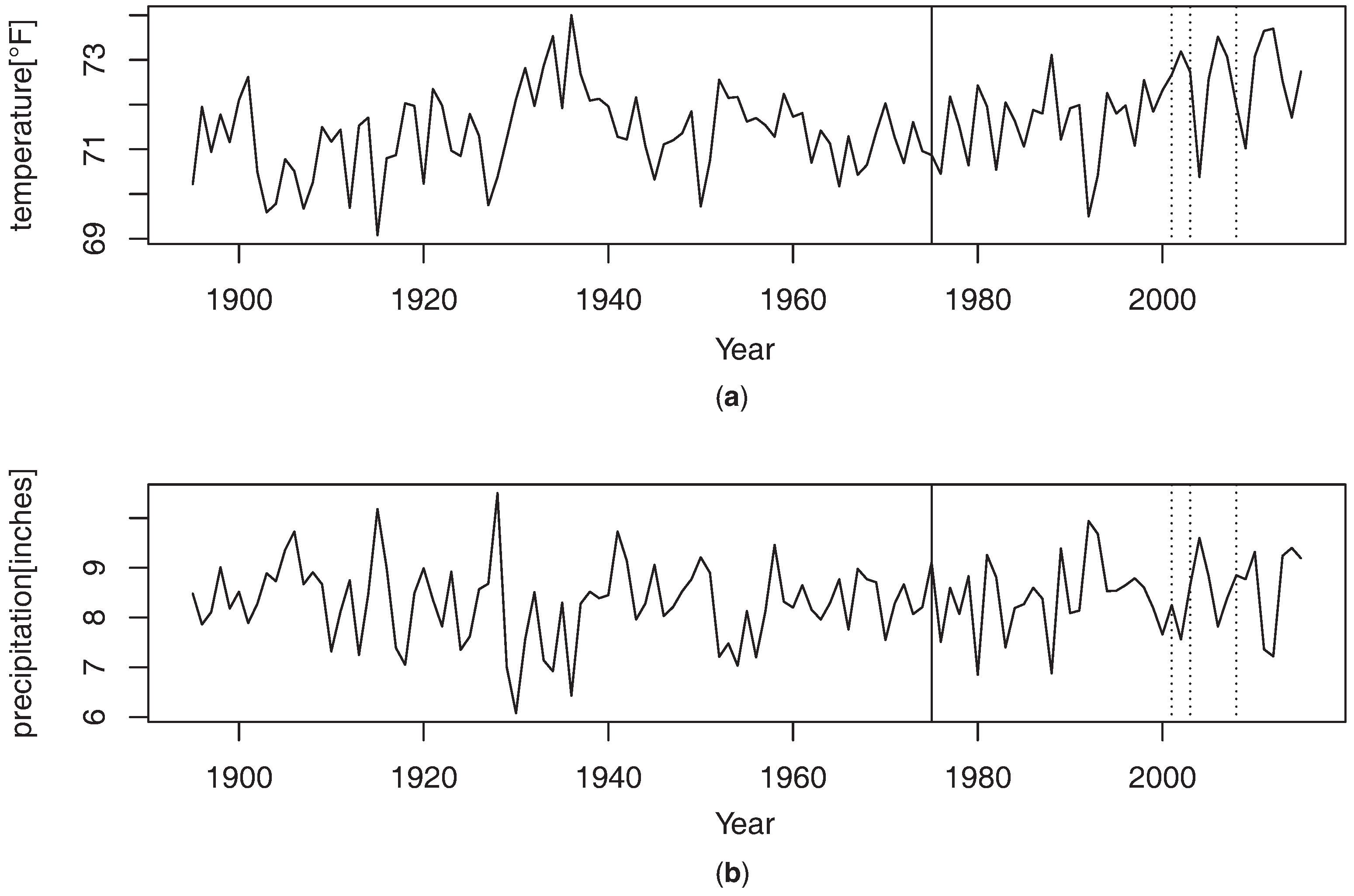
4.2. Real Data Analysis

In this section, we illustrate an example of a real data analysis. We consider bivariate climate data consisting of temperature and precipitation over the contiguous United States. There is a lot of literature studying the association of temperature and precipitation over the United States, and they reported empirical evidence that there is an obvious relationship between two variables (see Zhao and Khalil [35] and Huang and van Den Dool [36] and the papers cited therein). Recently, several authors have used a copula based methodology to model the joint distribution of temperature and precipitation (see, e.g., Favre et al. [37], Shiau et al. [38], Dupuis [39] and Schölzel and Friederichs [40]). However, the precedent studies only focus on the problem as to which copula model best fitted the empirical data. Here, we use the copula functions to model the dependence between temperature and precipitation and attempt to monitor for stability of dependence. Annual mean temperature and annual mean precipitation in summer months (June, July, and August) over the contiguous United States from 1895 to 2015 are used for empirical data. The data can be obtained from NOAA’s National Centers for Environmental Information (NCEI). Figure 1 shows that precipitation and temperature tend to be negatively correlated. It is well known that warmer summers usually result in drier conditions and colder summers are likely to be wetter. For historical data, the data from 1895 to 1975 is used, which has 81 observations. As discussed earlier, since the monitoring test for copula function can be influenced by a change in marginal distribution, the change point tests for marginal distributions are performed in advance of implementing the monitoring test for a copula function change. To this end, we perform the test of Lee et al. [22] who sequentially monitored marginal distributional changes based on the following test statistic:

$$D_{k,n}^D=\sqrt{n}\underset{-\infty \le z\le \infty }{sup}\left|F_{ik}(z)-F_{in}(z)\right|\mathrm{for}i=1,2,$$

where $F_{ik}$ is the empirical distribution based on the observation up to time k, while $F_{in}$ is the empirical distribution obtained based on the historical data. By observing new data sequentially, we first conduct the monitoring test for marginal distributional changes. If there are no changes in marginal distributions, we can perform the monitoring test for the copula function change. Since both of the two series detect no evidence of a change in marginal distributions at the nominal level 0.05, we apply monitoring procedure based on the test statistic in (7) to detect a change of dependence. For this task, we use the boundary function in (5) with $a=2$ and perform the bootstrap method in Section 3 with $B=500$. As a result, it appears that the test detects a change in dependence at nominal levels 0.01, 0.05, and 0.10. The location of the stopping time is summarized in

Table 5. The stopping time.

α	$\widehat{\mathit{\tau }}(\mathit{n})$	Year
$0.01$	114	2008
$0.05$	109	2003
$0.10$	107	2001

and Figure 1 illustrates the stopping time in dependence: the solid line corresponds to the end of historical data and the dotted lines identify the detected stopping time.

5. Conclusions

In this study, we designed the monitoring test for a change of copula function on the basis of the empirical copula functions. The test is shown to have its limiting distribution as the supremum of the Kiefer process under certain regularity conditions. The simulation results reported in Section 4 confirms that our test performs adequately. Our method to monitor the change of copula function has several advantages. The procedure is copula model free and we use a bootstrap method to overcome the difficulty that the asymptotic limiting distribution depends on the unknown copula function. For this reason, it is directly applicable in practice even when we do not know the true copula function. Furthermore, finite sample properties are expected to be well behaved since we use a bootstrap method. Our monitoring test has been established under the assumption that each series of random vector is independent and identically distributed. However, this assumption is often violated in practice and one might be able to consider even a broader class of stochastic processes such as autoregressive moving average (ARMA), ARCH and GARCH processes. Recently, Doukhan et al. [41] and Bücher and Volgushev [42] considered the weak convergence of the empirical copula process under serial dependence. These studies form the basis for our new monitoring test for copula function under weak dependence. We leave the task of extending our test to future study.

References

1. Cherubini, U.; Luciano, E.; Vecchiato, W. Copula Methods in Finance; John Wiley & Sons: Hoboken, NJ, USA, 2004. [Google Scholar]
2. Cherubini, U.; Gobbi, F.; Mulinacci, S.; Romagnoli, S. Dynamic Copula Methods in Finance; John Wiley & Sons: Hoboken, NJ, USA, 2012. [Google Scholar]
3. McNeil, A.J.; Frey, R.; Embrechts, P. Quantitative Risk Management: Concepts, Techniques, and Tools; Princeton Series in Finance: London, UK, 2005. [Google Scholar]
4. Hougaard, P. Analysis of Multivariate Survival Data; Springer: Berlin/Heidelberg, Germany, 2000. [Google Scholar]
5. Longin, F.; Solnik, B. Is the correlation in international equity returns constant: 1960–1990? J. Int. Money Financ. 1995, 14, 3–26. [Google Scholar] [CrossRef]
6. Patton, A.J. Modelling asymmetric exchange rate dependence. Int. Econ. Rev. 2006, 47, 527–556. [Google Scholar] [CrossRef]
7. Rodriguez, J.C. Measuring financial contagion: A copula approach. J. Empir. Financ. 2007, 14, 401–423. [Google Scholar] [CrossRef]
8. Dias, A.; Embrechts, P. Change-point analysis for dependence structure in finance and insurance. In Risk Measures for the 21st Century; Szegoe, G., Ed.; John Wiley & Sons: Hoboken, NJ, USA, 2004; pp. 321–335. [Google Scholar]
9. Guegan, D.; Zhang, J. Change analysis of dynamic copula for measuring dependence in multivariate finance data. Quant. Financ. 2010, 10, 421–430. [Google Scholar] [CrossRef] [Green Version]
10. Harvey, C. Tracking a changing copula. J. Empir. Financ. 2010, 17, 485–500. [Google Scholar] [CrossRef]
11. Busetti, F.; Harvey, C. When is a copula constant? A test for changing relationships. J. Financ. Econom. 2011, 9, 106–131. [Google Scholar] [CrossRef]
12. Na, O.; Lee, J.; Lee, S. Change point detection in copula ARMA-GARCH Models. J. Time Ser. Anal. 2012, 33, 554–569. [Google Scholar] [CrossRef]
13. Quessy, J.F.; Saïd, M.; Favre, A.C. Multivariate Kendall’s tau for change-point detection in copulas. Can. J. Stat. 2013, 41, 65–82. [Google Scholar] [CrossRef]
14. Bücher, A.; Ruppert, M. Consistent testing for a constant copula under strong mixing based on the tapered block multiplier technique. J. Multivar. Anal. 2013, 116, 208–229. [Google Scholar] [CrossRef]
15. Bücher, A.; Kojadinovic, I.; Rohmer, T.; Segers, J. Detecting changes in cross-sectional dependence in multivariate time series. J. Multivar. Anal. 2014, 132, 111–128. [Google Scholar] [CrossRef]
16. Chu, C.S.J.; Stinchcombe, M.; White, H. Monitoring structural change. Econometrica 1996, 64, 1045–1065. [Google Scholar] [CrossRef]
17. Horváth, L.; Hušková, M.; Kokoszka, P.; Steinebach, J. Monitoring changes in linear models. J. Stat. Plan. Inference 2004, 126, 225–251. [Google Scholar] [CrossRef]
18. Berkes, I.; Gombay, E.; Horvárh, L.; Kokoszaka, P. Sequential change-point detection in GARCH(p,q) models. Econ. Theory 2004, 20, 1140–1167. [Google Scholar] [CrossRef]
19. Gombay, E.; Serban, D. Monitoring parameter change in AR(p) time series models. J. Multivar. Anal. 2009, 100, 715–725. [Google Scholar] [CrossRef]
20. Na, O.; Lee, Y.; Lee, S. Monitoring parameter change in time series models. Stat. Methods Appl. 2011, 20, 171–199. [Google Scholar] [CrossRef]
21. Na, O.; Lee, J.; Lee, S. Monitoring test for stability of copula parameter in time series. J. Korean Stat. Soc. 2014, 43, 483–501. [Google Scholar] [CrossRef]
22. Lee, S.; Lee, Y.; Na, O. Monitoring distributional changes in autoregressive models. Commun. Stat. 2009, 38, 2969–2982. [Google Scholar] [CrossRef]
23. Fermanian, J.D.; Radulović, D.; Wegkamp, M. Weak convergence of empirical copula processes. Bernoulli 2004, 10, 847–860. [Google Scholar] [CrossRef]
24. Rémillard, B.; Scaillet, O. Testing for equality between two copulas. J. Multivar. Anal. 2009, 100, 377–386. [Google Scholar] [CrossRef]
25. Bücher, A.; Dette, H. A note on bootstrap approximations for the empirical copula process. Stat. Probab. Lett. 2010, 80, 1925–1932. [Google Scholar] [CrossRef]
26. Bouzebda, S. On the strong approximation of bootstrapped empirical copula process with applications. Math. Methods Stat. 2012, 21, 153–188. [Google Scholar] [CrossRef]
27. Joe, H. Multivariate Models and Dependence Concepts; Chapman and Hall: London, UK, 1997. [Google Scholar]
28. Nelsen, R.B. An Introduction to Copulas; Springer: Berlin/Heidelberg, Germany, 2006. [Google Scholar]
29. Na, O.; Lee, J.; Lee, S. Change point detection in SCOMDY models. AStA Adv. Stat. Anal. 2013, 97, 215–238. [Google Scholar] [CrossRef]
30. Adler, R.J. An introduction to continuity, extrema, and related topics for general Gaussian processes. In Institute of Mathematical Statistics Lecture Notes; Monograph Series; Institute of Mathematical Statistics: Hayward, CA, USA, 1990; Volume 12, pp. 1–41. [Google Scholar]
31. Piterbarg, V.I. Asymptotic Methods in the Theory of Gaussian Processes and Fields; American Mathematical Society: Providence, RI, USA, 1996. [Google Scholar]
32. Csörgő, M.; Horváth, L. A note on strong approximations of multivariate empirical processes. Stoch. Process. Their Appl. 1988, 28, 101–109. [Google Scholar] [CrossRef]
33. Segers, J. Asymptotics of empirical copula processes under non-restrictive smoothness assumptions. Bernoulli 2012, 18, 764–782. [Google Scholar] [CrossRef]
34. Tsukahara, H. Empirical Copulas and Some Applications; Seijo University: Tokyo, Japan, 2000. [Google Scholar]
35. Zhao, W.; Khalil, M.A.K. The Relationship between Precipitation and Temperature over the Contiguous United States. J. Clim. 1992, 6, 1232–1236. [Google Scholar] [CrossRef]
36. Huang, J.; Van Den Dool, H.M. Monthly precipitation-temperature relations and temperature prediction over the United States. J. Clim. 1993, 6, 1111–1132. [Google Scholar] [CrossRef]
37. Favre, A.C.; Adlouni, S.E.; Perreault, L.; Thiémonge, N.; Bobée, B. Multivariate hydrological frequency analysis using copulas. Water Resour. Res. 2004, 40, 1–12. [Google Scholar] [CrossRef]
38. Shiau, J.T.; Feng, S.; Nadarajah, S. Assessment of hydrological droughts for the Yellow River, China, using copulas. Hydrol. Process. 2007, 21, 2157–2163. [Google Scholar] [CrossRef]
39. Dupuis, D.J. Using copulas in hydrology: Benefits, cautions, and issues. J. Hydrol. Eng. 2007, 12, 381–393. [Google Scholar] [CrossRef]
40. Schölzel, C.; Friederichs, P. Multivariate non-normally distributed random variables in climate research—Introduction to the copula approach. Nonlinear Process. Geophys. 2008, 15, 761–772. [Google Scholar] [CrossRef]
41. Doukhan, P.; Fermanian, J.D.; Lang, G. An empirical central limit theorem with applications to copulas under weak dependence. Stat. Inference Stoch. Process. 2009, 12, 65–87. [Google Scholar] [CrossRef]
42. Bücher, A.; Volgushev, S. Empirical and sequential empirical copula processes under serial dependence. J. Multivar. Anal. 2013, 119, 61–70. [Google Scholar] [CrossRef]
Figure 1. Annual mean temperature and annual mean precipitation in summer months over the contiguous United States from 1895 to 2015. (a) Annual mean temperature in summer; (b) Annual mean precipitation in summer.
Entropy 18 00457 g001