
Information-Theoretic Analysis of Memoryless Deterministic Systems

1
Institute for Communications Engineering, Technical University of Munich, Munich 80290, Germany
2
Signal Processing and Speech Communication Laboratory, Graz University of Technology, Graz 8010, Austria
*
Author to whom correspondence should be addressed.
Entropy 2016, 18(11), 410; https://doi.org/10.3390/e18110410
Submission received: 18 August 2016
/
Revised: 27 October 2016
/
Accepted: 14 November 2016
/
Published: 17 November 2016
(This article belongs to the Section Information Theory, Probability and Statistics)
Abstract
:The information loss in deterministic, memoryless systems is investigated by evaluating the conditional entropy of the input random variable given the output random variable. It is shown that for a large class of systems the information loss is finite, even if the input has a continuous distribution. For systems with infinite information loss, a relative measure is defined and shown to be related to Rényi information dimension. As deterministic signal processing can only destroy information, it is important to know how this information loss affects the solution of inverse problems. Hence, we connect the probability of perfectly reconstructing the input to the information lost in the system via Fano-type bounds. The theoretical results are illustrated by example systems commonly used in discrete-time, nonlinear signal processing and communications.
1. Introduction
When opening a textbook on linear [1] or nonlinear [2] deterministic signal processing, input-output systems are typically characterized—aside from the difference or differential equation defining the system—by energy- or power-related concepts: or energy/power gain, passivity, losslessness, input-output stability, and transfer functions are all defined using the amplitudes (or amplitude functions like the squared amplitude) of the involved signals, therefore essentially energetic in nature. When opening a textbook on statistical signal processing [3] or an engineering-oriented textbook on stochastic processes [4], one can add correlations, power spectral densities, and how they are affected by linear and nonlinear systems (e.g., the Bussgang theorem [4] (Theorem 9-17)). By this overwhelming prevalence of energy concepts and second-order statistics, it is no surprise that many signal processing problems are formulated in terms of energetic cost functions, e.g., the mean squared error. What these books are currently lacking is an information-theoretic characterization of signal processing systems, despite the fact that such a characterization is strongly suggested by the data processing inequality [5] (Corollary 7.16): We know that the information content of a signal (be it a random variable or a stochastic process) cannot increase by deterministic processing, just as, loosely speaking, a passive system cannot increase the energy contained in a signal.
The information lost in a system not only depends on the system, but also on the signal carrying this information; the same holds for the energy lost or gained. There is a strong connection between energy and information for Gaussian signals: Entropy and entropy rate of a Gaussian signal are directly related to its variance and power spectral density, respectively. For non-Gaussian signals, such as they appear in nonlinear systems, this connection between energy and information is less immediate. Both variance and entropy depend on the distribution of the signal, and neither can be used to compute the other—at best, using the variance a bound on the entropy can be computed by the max-entropy property of the Gaussian distribution. In nonlinear systems, that typically involve non-Gaussian signals, energy and information therefore behave differently.
While we have a definition of the energy loss (namely, the inverse gain), an analysis of the information loss in a system has not been presented yet. This gap is even more surprising since important connections between information-theoretic quantities and signal processing performance measures have long been known: The mutual information between a random variable and its noisy observation is connected to the minimum mean squared reconstruction error (MSRE) [6], and mutual information presents a tight bound on the gain for nonlinear prediction [7]. It is the purpose of this work to close this gap and to propose information loss as a general system characteristic, complementing the prevailing energy-centered descriptions. We therefore define absolute and relative information loss and analyze their elementary properties in Section 2.
On more general terms, prediction and reconstruction are inverse problems, i.e., problems for which typically more than one solution exists or for which the solution is unstable with respect to (w.r.t.) the available data. Nevertheless, given certain assumptions or constraints on the solution, reconstruction is at least partly possible. For example, a quantizer maps intervals to a discrete set of real numbers, and choosing these representing numbers appropriately reduces the MSRE. That in this case perfect reconstruction is impossible is not only intuitive, but will be proved in Section 4 by arguing that an infinite amount of information is lost (cf. Corollary 2 and Proposition 4) and by showing that this leads to a reconstruction error probability of 100% (Proposition 11).
Not all inverse problems prohibit perfect reconstruction. Consider the rectifier in Figure 1: Given an arbitrary output value, there are exactly two possible corresponding input values; we are lacking one bit of information about the input by observing the output, at least if positive and negative input values are equally probable (see Section 5.4). Hence, the probability of perfectly reconstructing the input is 50%. Furthermore, while the information loss does not depend on the actual output value, the MSRE does: The larger the output value, the larger the MSRE caused by rectifying the signal. This toy example thus beautifully illustrates the inherent difference between the concepts of information and energy/power, and suggests the usefulness of a signal processing theory built upon the former. In Section 3 we quantify the information loss for a class of systems for which reconstruction is an inverse problem with at most countably many possible solutions. While we do not provide methods to solve these inverse problems, we provide bounds on their optimal performance: Information, once lost, cannot be recovered, hence information loss bounds the reconstruction error probability as we show in Proposition 9.
Our analysis focuses on a relatively small class of systems: Memoryless systems described by multivariate and/or vector-valued functions, i.e., systems operating on (multi-dimensional) random variables. Already this small class poses a multitude of questions (e.g., what happens if we lose an infinite amount of information?), to some of which we present adequate answers (e.g., by the introduction of a relative measure of information loss). The presented results can be regarded as a first small step towards a system theory from an information-theoretic point-of-view; we suggest possible future steps in the outlook in Section 6.
To illustrate the practical relevance of our theoretical results, in Section 5 we apply them to systems from signal processing and communications as diverse as principal components analysis, energy detection receivers, quantizers, and center clippers. Given the focus of this work, it is neither intended nor possible to investigate these systems in great detail. Rather, they act as examples for what is possible with the developed theory, and what surprising results can be obtained by looking at these systems from an information-theoretic point-of-view.
While some parts of our results have appeared elsewhere [8,9,10], aside from the first author’s dissertation [11] this is the first time they are presented collectively. Additionally, the Fano-type inequalities between the relative and absolute measures of information loss and the probability of a reconstruction error are altogether new.
Related Work
To the best of the authors’ knowledge, very few results have been published about the information processing behavior of deterministic input-output systems. Notable exceptions are Pippenger’s analysis of the information lost in the multiplication of two integer random variables [12] and the work of Watanabe and Abraham concerning the rate of information loss caused by feeding a discrete-time, finite-alphabet stationary stochastic process through a non-injective function [13]. Moreover, in [14], the authors made an effort to extend the results of Watanabe and Abraham to input-output systems with finite internal memory. All these works, however, focus only on discrete random variables and stochastic processes.
In his seminal work, Shannon investigated the entropy loss in a linear filter [15] (Theorem 14 in Section 22). Filtering a stochastic process with a filter characteristic changes the process’ differential entropy rate by
where W is the bandwidth of the stochastic process. Since Shannon considered passive filters, i.e., , he called this change of differential entropy rate an entropy loss. This entropy loss is a consequence of the fact that differential entropy is not invariant under an invertible coordinate transform; It is not suitable to measure the reduction of the available information in non-negative bits as we do in this work.
Sinanović and Johnson proposed a system theory for neural information processing in [16]. Their assumptions (information need not be stochastic, the same information can be represented by different signals, information can be seen as a parameter of a probability distribution, etc.) suggest the use of the Kullback–Leibler divergence as a central quantity, and are hence in the spirit of Akaike’s work on statistical model identification. Akaike proposed using the Kullback–Leibler divergence as a loss function, albeit in the sense of estimation theory [17], and thus extended the maximum likelihood principle. His information-theoretic method was applied in time series analysis, e.g., in determining the coefficients and the order of a fitted autoregressive model [18] (Section VI).
Finally, system design based on information-theoretic cost functions has recently received some attention: The information bottleneck method [19] (using information loss as a cost function, cf. [11] (p. 108)), originally developed for machine learning, has been adapted for signal processing problems such as speech enhancement [20,21] and quantizer design [22]. The error entropy has been successfully used in the adaptation of nonlinear adaptive systems [23]. Similarly, the entropy of a complex Gaussian error reveals more about its second-order statistics than its variance does, hence linear adaptive filters optimized according to this entropy perform better than those minimizing the mean squared error [24]. On a broader definition, information-theoretic system design also subsumes rate-distortion theory, i.e., the design of systems that transfer a minimal amount of information in order to allow reconstruction of the input subject to a maximum distortion [25] (Chapter 10).
Another canonical information-theoretic topic related to our work are strong data processing inequalities. Loosely speaking, and with the terminology from Section 4, they deal with determining a lower bound on the relative information loss caused by a stochastic channel. Unlike in our work, the strong data processing inequality is a property of the channel alone and does not depend on the input statistics. For further information on strong data processing inequalities, the reader is referred to [26] and the references therein.
2. Definition and Elementary Properties of Information Loss and Relative Information Loss
2.1. Notation and Preliminaries
Since the systems we deal with in this work are described by nonlinear functions, we use the terms “systems” and “functions” interchangeably. We adopt the following notation: Random variables (RVs) are represented by upper case letters (e.g., X), lower case letters (e.g., x) are reserved for (deterministic) constants or realizations of RVs. The alphabet of an RV is indicated by a calligraphic letter (e.g., ) and is always assumed to be a subset of an N-dimensional Euclidean space , for some N. The probability measure of an RV X is denoted by . If is a proper subset of the N-dimensional Euclidean space and if is absolutely continuous w.r.t. the N-dimensional Lebesgue measure (in short, ), then possesses a probability density function (PDF), which we will denote as .
We deal with functions of RVs: If, for example, is measurable and B a measurable set, we can define a new RV as with probability measure
where denotes the preimage of B under g. Abusing notation, we write for the probability measure of a single point instead of .
We also need the notion of a uniform quantizer that partitions into hypercubes with edges of length . We thus define
where the floor operation is applied element-wise if X is a multi-dimensional RV. The partition induced by this uniform quantizer will be denoted as , e.g., for a one-dimensional RV, the k-th element of is . Note that the partition gets refined with increasing n.
Finally, , , , and denote the entropy, the differential entropy, the binary entropy function, and the mutual information, respectively. Unless noted otherwise, the logarithm is taken to base two, so all entropies are measured in bits.
We will deal with both discrete and non-discrete RVs. The result [5] (Lemma 7.18)
allows us to compute the entropy also for non-discrete (e.g., continuous) RVs; for example, the entropy of an RV X with an absolutely continuous probability measure satisfies .
Similarly, the mutual information between two RVs X and Z with joint probability measure on can be computed as [5] (Lemma 7.18)
where also is partitioned into . Again, this equation allows computing the mutual information between arbitrary RVs. In the common case where both X and Z are discrete with finite entropy, one gets ; if X and Z have a joint PDF, then . Finally, if X is discrete with a finite alphabet and Z is arbitrary, then [5] (Lemma 7.20)
2.2. Information Loss
A measure of information loss in a deterministic input-output system should, roughly speaking, quantify the difference between the information available at its input and its output. While for discrete, finite-alphabet RVs this amounts to the difference of their entropies, continuous RVs require more attention. To this end, in Figure 2a, we propose a model to compute the information loss of a system which applies to all real-valued RVs.
In particular, we quantize the system input with partition and compute the mutual information between the input X and its quantization , as well as the mutual information between the system output Y and . The first quantity is an approximation of the information available at the input and observable at resolution , while the second approximates the information shared between input and output, i.e., the information passing through the system and thus being available at its output (also observable at resolution ). By the data processing inequality [5] (Corollary 7.16), the former cannot be smaller than the latter, i.e., , with equality if the system is described by a bijective function. We compute the difference between these two mutual informations to obtain an approximation of the information lost in the system:
With (6) one obtains
For every , we have , hence also . Moreover, by the data processing inequality, for every , we have that monotonically. Applying the monotone convergence theorem thus allows us to write
With this in mind, we present:
Definition 1 (Information Loss).
Let X be an RV with alphabet and let . The information loss induced by g is
This definition has recently been justified by an axiomatization of information loss [27]. For a discrete input RV X we obtain . Moreover, for bijective functions the information loss vanishes: Bijective functions describe information lossless systems. In what follows we will stick to the notation rather than to to make clear that Y is a function of X.
For discrete input RVs X or stochastic systems (e.g., communication channels with noise) the mutual information between the input and the output , i.e., the information transfer, is an appropriate characterization. In contrast, deterministic systems with non-discrete input RVs usually exhibit infinite information transfer . As we will show in Section 3, there exists a large class of systems for which the information loss remains finite, thus allowing to give a meaningful description of the system.
One elementary property of information loss, which will prove useful in developing a system theory from an information-theoretic point-of-view, applies to cascades of systems (see Figure 2b).
Proposition 1 (Information Loss of a Cascade).
Consider two functions and and a cascade of systems implementing these functions. Let and . The information loss induced by this cascade, or equivalently, by the system implementing the composition is given by:
This result shows a beautiful symmetry to the cascade of linear filters and , for which the logarithmic transfer function is a sum of the individual logarithmic transfer functions:
While for stable, linear filters the order of the cascade is immaterial, the order of non-linear systems matters in terms of information loss. Consequently, while post-processing cannot recover information already lost, pre-processing can prevent it from getting lost, cf. [28]. Therefore, information theory was shown to be especially useful in designing pre-processing systems, e.g., filters prior to (down-)sampling [29] or linear transforms prior to dimensionality reduction ([30] (Section V), [31]).
Proof.
Referring to Definition 1 and [32] (Chapter 3.9) we obtain
since is a Markov tuple. ☐
A sufficient condition for the information loss to be infinite is presented in:
Proposition 2
(Infinite Information Loss, [8] (Theorem 5)). Let , , and let the input RV X be such that its probability measure has an absolutely continuous component which is supported on . If there exists a set of positive -measure such that the preimage is uncountable for every , then
A simple example of a system with an uncountable preimage is the quantizer, which maps quantization intervals to points. In most practical cases the input has a continuously distributed component (e.g., due to Gaussian noise). The output alphabet is a finite (or countable) set, of which at least one element will have positive -probability. The preimage of this element is the corresponding quantization interval, an uncountable set. The quantizer converts an infinite-information input signal to a finite-information output signal—the information loss is infinite (cf. Section 5.1).
2.3. Relative Information Loss
As we just saw, the quantizer belongs to a class of systems with finite information transfer and infinite information loss. In contrast, Section 3 deals with systems that transfer an infinite amount of information but lose only a finite amount. In addition to these classes, there are systems for which both information transfer and information loss are infinite. For these systems, a different characterization is necessary, which leads to:
Definition 2 (Relative Information Loss).
The relative information loss induced by is defined as
provided the limit exists.
Due to the non-negativity of entropy and the fact that conditioning reduces entropy, we always have . More interestingly, the relative information loss is related to the Rényi information dimension:
Definition 3
(Rényi Information Dimension [33]). The information dimension of an RV X is
provided the limit exists and is finite.
We adopted this definition from Wu and Verdú, who showed in [34] (Proposition 2) that it is equivalent to the one given by Rényi in [33]. We also excluded the case that the information dimension is infinite, which may occur if [34] (Proposition 1). Conversely, if the information dimension of an RV X exists, it is guaranteed to be finite if [33] or if for some [34]. Aside from that, the information dimension exists for discrete RVs and RVs with probability measures absolutely continuous w.r.t. the Lebesgue measure on a sufficiently smooth manifold [33], for mixtures of RVs with existing information dimension [33,34,35], and self-similar distributions generated by iterated function systems [34]. Finally, the information dimension exists if the MMSE dimension exists [36] (Theorem 8). For the remainder of this work we will assume that the information dimension of all considered RVs exists and is finite.
We are now ready to state:
Proposition 3
(Relative Information Loss and Information Dimension, [11] (Proposition 2.8)). Let X be an N-dimensional RV with positive information dimension and finite . If and exists -a.s., then the relative information loss equals
where .
A consequence of this definition is that relative information loss is largely independent of the shape of a continuous distribution, unless it influences its information dimension. In particular, if has an N-dimensional PDF , then regardless of the shape of the PDF.
2.4. Interplay between Information Loss and Relative Information Loss
We introduced the relative information loss to characterize systems for which the absolute information loss from Definition 1 is infinite. The following result shows that, at least for input RVs with infinite entropy, an infinite absolute information loss is a prerequisite for positive relative information loss:
Proposition 4
(Positive Relative Loss leads to Infinite Absolute Loss, [11] (Proposition 2.9)). Let X be such that and let . Then, .
Note that the converse is not true: There exist examples where an infinite amount of information is lost, but for which the relative information loss nevertheless vanishes [11] (Example 4).
3. Information Loss for Piecewise Bijective Functions
In this section we analyze the information loss for a restricted class of systems and under the practically relevant assumption that the input RV has a probability distribution supported on . Let be a finite or countable partition of and let for all i. We present
Definition 4 (Piecewise Bijective Function).
A piecewise bijective function , , is a surjective function defined in a piecewise manner:
where each is bijective. Furthermore, the Jacobian matrix exists on the closures of , and its determinant, , is non-zero -a.s.
A direct consequence of this definition is that also . Thus, possesses a PDF that, using the method of transformation (e.g., [4] (p. 244)), can be computed as
Since the preimage is countable for all , it follows that . With from we can apply Proposition 3 to obtain . Thus, relative information loss will not tell us much about the behavior of the system. In the following, we therefore stick to Definition 1 and analyze the (absolute) information loss in piecewise bijective functions (PBFs).
3.1. Information Loss in PBFs
Proposition 5
(Information Loss and Differential Entropy, [11] (Theorem 2.2)). The information loss induced by a PBF is given as
where the expectation is taken w.r.t. X.
We want to point out that, despite the input X being a continuous RV, the computation of is meaningful. With reference to (6), conditioned on , the input X is a discrete RV taking values in the at most countable preimage . Therefore, one can compute
where the term inside the integral is the entropy of a discrete RV.
Aside from being one of the main results of our theory, it also extends a result presented in [4] (p. 660). There, it was claimed that
with equality if and only if g is bijective, i.e., a lossless system. The inequality results from
with equality if and only if g is invertible at x. Proposition 5 essentially states that the difference between the right-hand side and the left-hand side of (23) is the information lost due to data processing.
We note in passing that the statement of Proposition 5 has a tight connection to the theory of iterated function systems. In particular, Wiegerinck and Tennekes [37] analyzed the information flow in one-dimensional maps, which is the difference between information generation via stretching (corresponding to the term involving the Jacobian determinant) and information reduction via folding (corresponding to information loss). Ruelle [38] later proved that for a restricted class of iterated function systems the folding entropy cannot fall below the information generated via stretching if X has a measure that is ergodic w.r.t. g, and established a connection to the Kolmogorov–Sinaï entropy rate.
3.2. Upper Bounds on the Information Loss
Since the expressions in Proposition 5 may involve the logarithm of a sum, it is desirable to accompany the exact expressions by bounds that are easier to compute.
Proposition 6
(Tight Upper Bounds on Information Loss, [11] (Proposition 2.4)). The information loss induced by a PBF can be upper bounded by the following ordered set of inequalities:
where is the cardinality of the set B.
Two non-trivial scenarios, where these bounds hold with equality, are worth mentioning: First, for functions equality holds if the function is related to the cumulative distribution function of the input RV such that, for all x, (see extended version of [10]). The second scenario occurs when both function and PDF are “repetitive” in the sense that their behavior on is copied to all other , and that, thus, and in (20) are the same for all elements of the preimage . An example is a square-law device fed with a zero-mean Gaussian input (cf. Section 5.4).
3.3. Reconstruction and Reconstruction Error Probability
We now investigate connections between the information lost in a system and the probability of correctly reconstructing the system input, i.e., the application of information loss to inverse problems. In particular, we present a series of Fano-type inequalities between the information loss and the reconstruction error probability.
Intuitively, one expects that the fidelity of a reconstruction of a real-valued, continuous input RV is best measured by some distance measure “natural” to the set , such as, e.g., the mean absolute distance or the MSRE. However, as the discussions around Figure 1 and in Section 5.1 show, there is no connection between the information loss and such distance measures. Moreover, a reconstructor trying to minimize the MSRE differs from a reconstructor trying to perfectly recover the input signal with at least some probability. Since for piecewise bijective functions a perfect recovery of X is possible (in contrast to noisy systems, where this is not the case), in our opinion a thorough analysis of such reconstructors is in order.
Aside from being of theoretical interest, there are practical reasons to justify the investigation: As already mentioned in Section 3.2, the information loss is a quantity which is not always computable in closed form. If one can thus define a (sub-optimal) reconstruction of the input for which the error probability is easy to calculate, the Fano-type bounds would yield yet another set of upper bounds on the information loss. But also the reverse direction is of practical interest: Given the information loss of a system, the presented inequalities allow one to bound the reconstruction error probability . For example, the IEEE 802.15.4a standard features a semi-coherent transmission scheme combining pulse-position modulation and phase-shift keying to serve both coherent and non-coherent receivers (e.g., energy detectors, cf. Section 5.6) [39]. Although a non-coherent receiver has no access to the phase information, quantifying the resulting information loss allows to bound the probability of correctly reconstructing the information bits modulating the phase.
We therefore present Fano-type inequalities to bound the reconstruction error probability via information loss. Due to the peculiarities of entropy pointed out in [40], we restrict our attention to PBFs with finite partitions , guaranteeing a finite preimage for every output value.
Definition 5 (Reconstructor & Reconstruction Error).
Let be a reconstructor. Let E denote the event of a reconstruction error, i.e.,
The probability of a reconstruction error is given by
where .
In the following, we will focus on the maximum a posteriori (MAP) reconstructor; a sub-optimal reconstructor, which in many cases is easier to evaluate, has been presented and analyzed in [11] (Section 2.3.3). The MAP reconstructor chooses the reconstruction such that its conditional probability given the output is maximized, i.e.,
In other words, with Definition 5, the MAP reconstructor minimizes . Interestingly, this reconstructor has a simple description for the problem at hand:
Proposition 7 (MAP Reconstructor).
The MAP reconstructor for a PBF is
where
Proof.
We now derive Fano-type bounds for the MAP reconstructor, or any reconstructor for which . Under the assumption of a finite partition , Fano’s inequality [25] (p. 39) holds by substituting the cardinality of the partition for the cardinality of the input alphabet:
In the equation above one can exchange by to improve the bound. In what follows, we aim at further improvements.
Definition 6 (Bijective Part).
Let be the maximal set such that g restricted to this set is injective, and let be the image of this set. Thus, bijectively, where
Then denotes the bijectively mapped probability mass.
Proposition 8 (Fano-Type Bound).
For the MAP reconstructor—or any reconstructor for which —the information loss in a PBF is upper bounded by
Proof.
See Appendix A. ☐
If we compare this result with Fano’s original bound (33), we see that the cardinality of the partition is replaced by the expected cardinality of the preimage. Due to the additional term this improvement is only potential, since there exist cases where Fano’s original bound is better. An example is the third-order polynomial which we investigate in Section 5.5.
For completeness, we want to mention that for the MAP reconstructor also a lower bound on the information loss can be given. We restate:
Proposition 9
(Feder and Merhav [41]). The information loss in a PBF is lower bounded by the error probability of a MAP reconstructor via
where is a piecewise linear function defined as
for .
To the best of our knowledge, this bound cannot be improved for the present context since the cardinality of the preimage has no influence on .
4. Information Loss for Systems that Reduce Dimensionality
We now analyze systems for which the absolute information loss is infinite. This includes cases where the dimensionality—to be more precise, the information dimension—of the input signal is reduced, e.g., by dropping coordinates or by keeping the function constant on a subset of its domain.
Throughout this section we assume that and , thus and . We further assume that the function g describing the system is such that the relative information loss is positive, from which follows; cf. Proposition 4.
4.1. Relative Information Loss for Continuous Input RVs
For the sake of simplicity, we will consider only functions which are described by projections. The results can be easily generalized to cascades of projections and bi-Lipschitz functions, since the latter do not affect the information dimension of an RV [42] (Remark 28.9).
Proposition 10 (Relative Information Loss in Dimensionality Reduction).
Let be a partition of into K subsets. Let g be such that are projections to coordinates and let . Then, the relative information loss is
Proof.
See Appendix B. ☐
Corollary 1.
Let g be a projection of X onto M of its coordinates and let . Then, the relative information loss is
Corollary 2.
Let g be constant on a set with positive -measure, where . Let furthermore g be such that for all . Then, the relative information loss is
Prime examples for these two corollaries are the quantizer (Section 5.1), the center clipper (Section 5.2) and principal components analysis with dimensionality reduction (Section 5.7). The somewhat surprising consequence of these results is that the shape of the PDF has no influence on the relative information loss; whether the PDF is peaky in the clipping region or flat, or whether the omitted coordinates are highly correlated to the preserved ones neither increases nor decreases the relative information loss.
4.2. Reconstruction and Reconstruction Error Probability
We next take up the approach of Section 3.3 and present a relation between the relative information loss and the reconstruction error probability. Although the dimensionality of the data is reduced, the error event is still defined as . While for piecewise bijective functions the error probability was always bounded away from one by the fact that is at most countable for every , for functions that reduce the dimensionality of the data there can be for which . An example that can nevertheless benefit from such an analysis is the center clipper, which admits perfect reconstruction of all input values outside the clipping region (see Section 5.2). Even more relevant is this connection between relative information loss and the reconstruction error probability for compressed sensing [34,43]. While we still restrict our attention to the case and , Geiger [11] (Section 2.4) generalizes this to arbitrary RVs with positive information dimension.
Proposition 11.
Let X be an N-dimensional RV with a probability measure supported on a compact set . Then, the error probability bounds the relative information loss from above, i.e.,
Proof.
See Appendix C. ☐
5. Some Examples from Signal Processing and Communications
In the previous sections we have developed several results about the information loss—absolute or relative—caused by deterministic systems. In this section we apply these results to a rather diverse selection of memoryless systems. We chose breadth rather than depth to best illustrate the various consequences of our theory.
5.1. Quantizer
We start with the information loss of a uniform scalar quantizer that is described by the function
With the notation introduced above we obtain . Assuming that X has a PDF, there will be at least one point for which . The conditions of Proposition 2 are thus fulfilled with and we obtain
This simple example illustrates the information loss as the difference between the information available at the input and the output of a system: While in all practically relevant cases a quantizer will have finite information at its output (), the information at the input is infinite as soon as has a continuous component. Moreover, assuming , even 100% of the information is lost: Since the quantizer is constant -a.s., we obtain with Corollary 2
Note that this does not immediately make quantizers useless: Quantizers still transfer a finite amount of information to the output. The task of the signal processing engineer is to design the quantizer (or the pre-processing system) such that this transferred information contains what is relevant for the receiver (cf. Section 5.7 and Section 6). If, for example, the input to the quantizer is a binary data signal superimposed with Gaussian noise, proper quantization can transfer a lot of the information about the data to the output while still destroying an infinite amount of (useless) information about the noise. Our measures of information loss make clear the point that quantizer design based on the input distribution alone is futile from an information-theoretic perspective. Quantizer design can be justified information-theoretically only if knowledge about the relevant signal components is available.
Combining (44) and Proposition 11, we can see that perfect reconstruction of the input is impossible. This naturally holds for all n, so a finer partition can neither decrease the relative information loss nor the reconstruction error probability. In contrast, the MSRE decreases with increasing n. Hence, relative information loss does not permit a direct interpretation in energy terms, again underlining the intrinsically different behavior of information and energy measures.
5.2. Center Clipper
While for a quantizer the mutual information between the input and the output may be an appropriate, because finite, characterization, the following example shows that also mutual information has its limitations.
The center clipper, used for, e.g., residual echo suppression [44], can be described by the following function (see Figure 3):
On the one hand, assuming and , with Proposition 2 the information loss becomes infinite. On the other hand, an infinite amount of information is shared between the input outside the clipping region and the output: It can be shown with [32] (Theorem 2.1.2) that
Relative information loss, however, does the trick: According to Corollary 2, one has . Moreover, since the function is invertible for , the reconstruction error probability satisfies ; hence, Proposition 11 is tight.
5.3. Adding Two RVs
Consider two N-dimensional input RVs and , and assume that the output of the system under consideration is given as the sum of these two RVs, i.e.,
We start by assuming that and have a joint probability measure . It can be shown that by transforming invertibly to and dropping the second coordinate we get
Different results may appear if the joint probability measure is supported on some lower-dimensional submanifold of . Consider, e.g., the case where , thus , and . As yet another example, assume that both input variables are one-dimensional, and that . Then, as it turns out,
which is a piecewise bijective function. As the analysis in Section 5.5 shows, in this case.
5.4. Square-Law Device and Gaussian Input
We now illustrate Proposition 5 by assuming that X is a zero-mean, unit variance Gaussian RV and that . We switch in this example to measuring entropy in nats and compute the differential entropy of X as . The output Y is a -distributed RV with one degree of freedom, for which the differential entropy can be computed as [45]
where γ is the Euler-Mascheroni constant [46] (p. 3). The Jacobian determinant degenerates to the derivative, and using some calculus we obtain
Applying Proposition 5 we obtain an information loss of , which after changing the base of the logarithm amounts to one bit. Indeed, the information loss induced by a square-law device is always one bit if the PDF of the input RV has even symmetry [10]. The same holds for the rectifier .
5.5. Polynomials
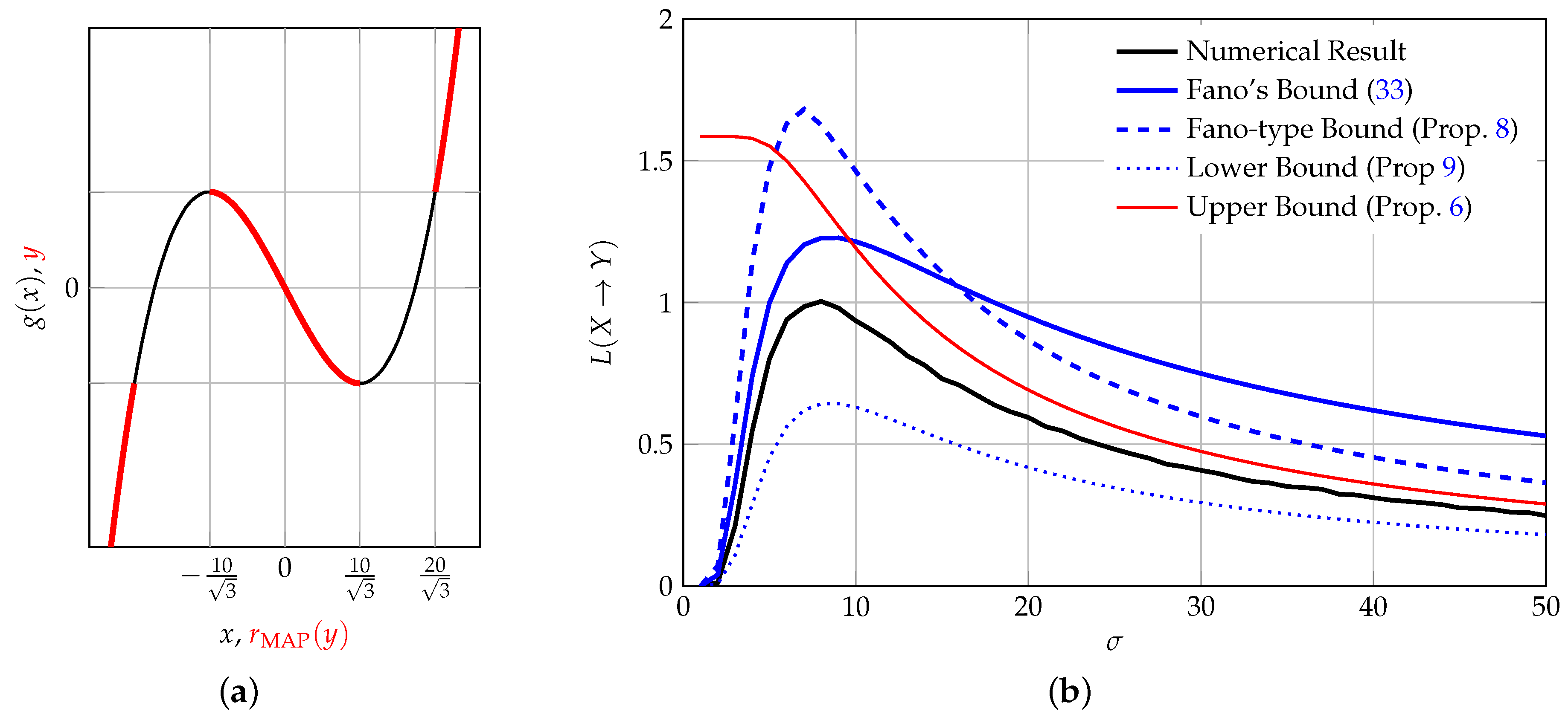
Consider the function depicted in Figure 4a, which is given as
The input to this function is a zero-mean Gaussian RV X with variance . A closed-form evaluation of the information loss is not possible, since the integral involves the logarithm of a sum. However, we note that
and thus , where Q denotes the Q-function [46] (Equation (26.2.3)). With a little algebra we thus obtain the bounds from Proposition 6 as
where .
It can be shown (the authors thank Stefan Wakolbinger for pointing us to this fact) that the MAP reconstructor assumes the properties depicted in Figure 4a, from which an error probability of
can be computed. We display Fano’s bound and the bounds from Propositions 6, 8 and 9 together with the information loss obtained by numerical simulations in Figure 4b. As it can be seen, the information loss increases with σ to a maximum value and then decreases again: On the one hand, for very small σ, most of the probability mass is contained in the interval , hence little information is lost (the input can be reconstructed with high probability). On the other hand, for large σ, more and more probability mass lies in areas in which the system is bijective (i.e., increases). Most of the information is lost for values around : At exactly these values, most of the information processing occurs. It is noteworthy that the bounds capture this information-processing nature of the system quite well. Moreover, this example shows that the bounds from Propositions 6 and 8 cannot form an ordered set; the same holds for Fano’s inequality, which can be better or worse than our Fano-type bound, depending on the scenario.
While this particular polynomial is just a toy example, it beautifully illustrates the usefulness of our theory: Polynomials are universal approximators of continuous functions supported on intervals (Weierstrass approximation theorem). Covering polynomials hence covers a large class of nonlinear memoryless systems, that are themselves important building blocks of (dynamical) Wiener and Hammerstein systems.
5.6. Energy Detection of Communication Signals
A Hammerstein system commonly used in communications is the energy detector, consisting of a square-law device followed by a integrate-and-dump circuit. We use this energy detector as a receiver for I/Q-modulated communication signals:
where is the carrier frequency. We assume that the in-phase and quadrature-phase symbols and have a symbol period of , which is an integer multiple of the carrier period . If and over one symbol period, then, for , we have
Let us assume that the symbol amplitudes A and B are coordinates of constellation points derived from quadrature amplitude modulation (QAM) or phase-shift keying (PSK). Specifically, suppose we are using 16-QAM, circular 16-QAM, and 16-PSK (see Figure 5)—we thus deal with a discrete input RV. It follows from (57) that Y preserves only the radius of the constellation points. Assuming that all constellation points are transmitted with equal probability, i.e., , this leads to the information loss calculated in Table 1. In particular, since in 16-PSK all constellation points have the same radius, all information is lost, . For a circular 16-QAM, the constellation points are distributed over four concentric circles, hence and . Finally, for 16-QAM the constellation points show three different radii, one of which has eight constellation points. The information loss in this case amounts to .
With pulse shaping, the information loss can be reduced. For example, suppose that sinusoidal pulses are used, i.e.,
where A and B are again coordinates of constellation points. If is an integer fraction of T and if , we get
where . For each symbol period , we thus obtain an output vector .
As it can be seen from (59), for , , and , for every we recover the scenario without pulse shapes, hence (57) and the corresponding information loss. For (and other, smaller, integration times), information loss can be reduced: Rather than having access to just the radius of the constellation point, the output is now a mixture of the sums and of the differences of squared amplitudes, and leads to the information loss shown in Table 1. Moreover, it can be shown that the information loss satisfies .
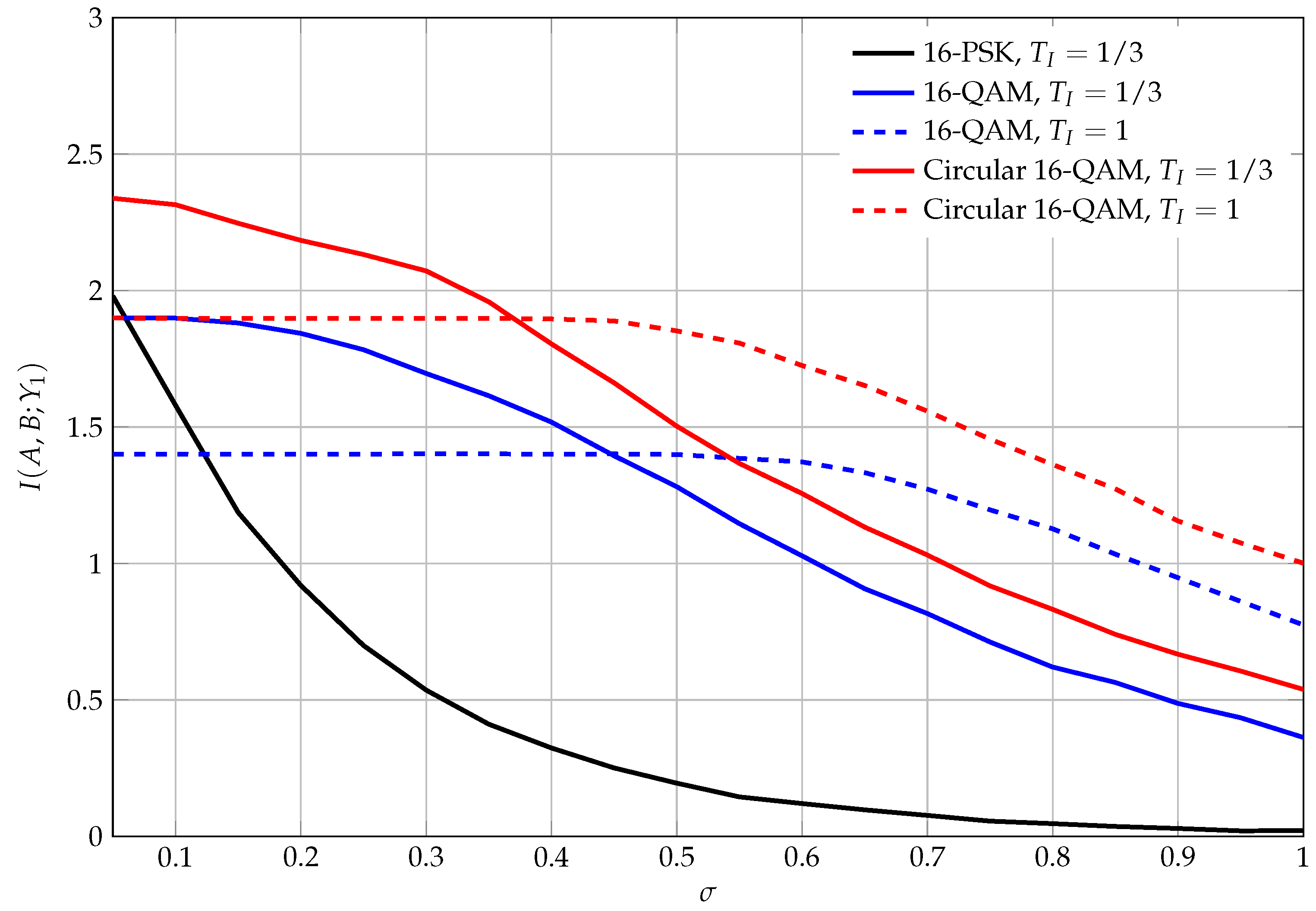
To illustrate these results, we performed numerical experiments. We investigated a discrete-time model where samples, samples, and where is either 100 or 300 samples. According to (58) we generated 1000 symbols for each constellation point depicted in Figure 5 and scaled A and B such that . We then added white Gaussian noise with a standard deviation of σ. The results of this experiment, in which we plot the mutual information , are shown in Figure 6. It can be seen that the mutual information approaches for small values of σ, but then decreases as the noise variance increases. Moreover, it can be seen that while the shorter integration time of causes less information loss for small noise variances, the performance drops quickly below the one for as the noise increases. This may be due to the fact that the reduced integration time limits the capabilities for noise averaging, but it may also be related to the fact that effectively more output symbols are available, which reduces the robustness of the scheme.
5.7. Principal Components Analysis and Dimensionality Reduction
Principal components analysis (PCA) exploits the eigenvalue decomposition of the data’s covariance matrix to arrive at a different representation of the input vector. This new representation should eventually allow to discard components corresponding to low variances. Indeed, performing PCA prior to dimensionality reduction preserves the subspace with the largest variance and minimizes the MSRE, where the reconstruction is based on the low-dimensional representation [31]. Thus, PCA is often applied in the hope that the most informative aspects of the input vector X are preserved. To analyze its information-theoretic properties—and to show that this hope is not well justified—we assume again that the input vector is an N-dimensional RV with .
Let be the matrix of eigenvectors of the input covariance matrix; then, PCA is defined as the following rotation:
Clearly, since is an orthogonal matrix, and . We now perform dimensionality reduction by preserving only the first coordinates of . Since the rotation of PCA is bi-Lipschitz and does not affect the information dimension of the rotated RVs, we get with Corollary 1
where Y contains the first M coordinates of . In comparison, reducing the dimensionality of the input vector without employing PCA leads to exactly the same relative information loss. Thus, without any additional knowledge about which aspect of the input data is relevant, PCA cannot be justified from an information-theoretic perspective. As soon as the relevant part of the information is known, the (relative or absolute) information loss in dimensionality reduction can be reduced by proper pre-processing [30]. If the relevant information is represented in the input data in a specific way, e.g., in a simple signal-and-noise model, PCA is the optimal pre-processing step [30] (Section V), [31].
Yet another example—PCA employing the sample covariance matrix—can be found in [9] (Section VI). There, it is shown that by rotating a data matrix into its own eigenspace, information is lost even without reducing the dimensionality of the data if the rotation matrix is not preserved. The information that is lost is that of the original orientation of the data matrix w.r.t. its eigenspace. Whether this information can be sacrificed or not strongly depends on the application: Performing sample covariance matrix-based PCA on signals coming from a microphone array, for example, might enhance the recorded signal, but completely destroys direction information.
6. Discussion and Outlook
In this work, we presented an information-theoretic framework to characterize the behavior of deterministic, memoryless input-output systems. In particular, we defined an absolute and a relative measure for the information loss occurring in a non-invertible system and linked these quantities to conditional entropy and Rényi information dimension. Our analysis of common signal processing systems showed that there is no apparent connection between these information-theoretic and prevailing energy-centered quantities, like the MSRE. In contrast, we were able to derive Fano-type inequalities between the information loss and the probability of a reconstruction error. Table 2 summarizes the results for some of the systems analyzed in Section 5 and again highlights the inherent difference between energy and information.
Future work will deal with extending the scope of our system theory and its applications to signal processing. The first issue that will be addressed is the fact that at present we are just measuring information “as is”; every bit of input information is weighted equally, and losing a sign bit amounts to the same information loss as losing the least significant bit in a binary expansion of a (discrete) RV. This fact leads to the apparent counter-intuitivity of some of our results, e.g., the fact that quantizers destroy 100% of the available information or that PCA cannot reduce the relative information loss caused by dimensionality reduction. Contrary to that, the literature employs information theory to prove the optimality of PCA in certain cases [31,47,48]—but see also [49] for conditions on the eigenvalue spectrum such that PCA is optimal for a certain signal-and-noise model. To build a bridge between our theory of information loss and the results in the literature, the notion of relevance has to be brought into game, allowing us to place unequal weights on different portions of the information available at the input. We proposed the corresponding notion of relevant information loss in [30], where we showed its applicability in signal processing and machine learning and, among other things, re-analyzed the optimality of PCA given a specific signal model. We furthermore showed that this notion of relevant information loss is fully compatible with what we presented in this paper.
Going from variances to power spectral densities, or, from information loss to information loss rates, represents the next step: If the input to our memoryless system is not a sequence of independent RVs but a discrete-time stationary stochastic process, how much information do we lose per unit time? Following [13], the information loss rate should be upper bounded by the information loss (assuming the marginal distribution of the process as the distribution of the input RV). Aside from a few preliminary results in [50] and an analysis of multirate signal processing systems in [29], little is known about this scenario, and we hope to bring some light into this issue in the future.
The next, bigger step is from memoryless to dynamical input-output systems: Referring to the discussion around (1), linear, time-invariant, stable, causal filters do not introduce any information loss and can be called information all-passes, cf. [11] (Lemma 5.2). In comparison to that, the class of nonlinear dynamical systems is significantly more difficult. We were able to present some results for discrete alphabets in [14]. For more general process alphabets we hope to obtain results for special subclasses, e.g., Volterra systems or affine input systems. For example, Wiener and Hammerstein systems, which are cascades of linear filters and static nonlinear functions, can completely be dealt with by generalizing our present work to stochastic processes.
While our theoretical results were developed mainly in view of a system theory, we believe that some of them will be of relevance also for analog compression, reconstruction of nonlinearly distorted signals, and chaotic iterated function systems.
Acknowledgments
This work was supported by the German Research Foundation (DFG) and the Technical University of Munich (TUM) in the framework of the Open Access Publishing Program. The authors thank Yihong Wu, Yale University, Siu-Wai Ho, Institute for Telecommunications Research, University of South Australia, and Tobias Koch, Dpto. de Toría de la Señal y Communicaciones, Universidad Carlos III de Madrid, for fruitful discussions and suggesting material. In particular, the authors wish to thank Christian Feldbauer, formerly Signal Processing and Speech Communication Laboratory, Graz University of Technology, for his valuable input during the work on Section 3.
Author Contributions
Both authors conceived and designed the analysis; Bernhard C. Geiger derived the results; Gernot Kubin contributed examples; Bernhard C. Geiger wrote the paper. Both authors have read and approved the final manuscript.
Conflicts of Interest
The authors declare no conflict of interest.
Abbreviations
The following abbreviations are used in this manuscript:
| MSRE | mean squared reconstruction error |
| RV | random variable |
| probability density function | |
| MMSE | minimum mean squared error |
| PBF | piecewise bijective function |
| MAP | maximum a posteriori |
| PCA | principal components analysis |
Appendix A. Proof of Proposition 8
The proof follows closely the proof of Fano’s inequality [25] (p. 38), where one starts with noticing that
The first term, can be upper bounded by , as in Fano’s inequality. However, also
since if and since otherwise. Thus,
For the second part note that , so we obtain
Upper bounding the entropy by we get
where is Jensen’s inequality ( acts as a PDF) and holds since and due to splitting the logarithm. This completes the proof.
Appendix B. Proof of Proposition 10
By assumption, is a projection, which preserves exactly of the N original coordinates. Assume, w.l.o.g., that the first coordinates are preserved, and that the remaining coordinates are dropped. It follows that , which is an -dimensional set. Moreover, the preimage of a set is given by
From immediately follows that , since the distribution of X possesses a PDF and the PDF of Y is obtained by marginalization. It needs to be shown that the distribution on the preimage of a singleton is absolutely continuous w.r.t. the -dimensional Lebesgue measure.
To this end, take such that , thus . Then, assume that there exists a with and, -a.s.,
Now, one can compute
while , which contradicts the assumption that . Consequently, , -a.s.
Appendix C. Proof of Proposition 11
Note that by the compactness of the quantized input has a finite alphabet, which allows us to employ Fano’s inequality
where
Since Fano’s inequality holds for arbitrary reconstructors, we let be the composition of the MAP reconstructor and the quantizer introduced in Section 2.1. Consequently, is the probability that and X do not lie in the same quantization bin. Since the bin volumes reduce with increasing n, increases monotonically to . We thus obtain with for
With the introduced definitions,
where is obtained by dividing both numerator and denominator by n and evaluating the limits: While , converges to the Minkowski-dimension of . The latter lies between and N, if [43] (Theorem 1 and Lemma 4), thus equals N. This completes the proof.
References
- Oppenheim, A.V.; Schafer, R.W. Discrete-Time Signal Processing, 3rd ed.; Pearson: Upper Saddle River, NJ, USA, 2010. [Google Scholar]
- Khalil, H.K. Nonlinear Systems, 3rd ed.; Pearson: Upper Saddle River, NJ, USA, 2000. [Google Scholar]
- Manolakis, D.G.; Ingle, V.K.; Kogon, S.M. Statistical and Adaptive Signal Processing; Artech House: London, UK, 2005. [Google Scholar]
- Papoulis, A.; Pillai, U.S. Probability, Random Variables and Stochastic Processes, 4th ed.; McGraw Hill: New York, NY, USA, 2002. [Google Scholar]
- Gray, R.M. Entropy and Information Theory; Springer: New York, NY, USA, 1990. [Google Scholar]
- Guo, D.; Shamai, S.; Verdú, S. Mutual Information and Minimum Mean-Square Error in Gaussian Channels. IEEE Trans. Inf. Theory 2005, 51, 1261–1282. [Google Scholar] [CrossRef]
- Bernhard, H.P. Tight Upper Bound on the Gain of Linear and Nonlinear Predictors. IEEE Trans. Signal Process. 1998, 46, 2909–2917. [Google Scholar] [CrossRef]
- Geiger, B.C.; Kubin, G. On the Information Loss in Memoryless Systems: The Multivariate Case. In Proceedings of the International Zurich Seminar on Communications (IZS), Zurich, Switzerland, 29 February–2 March 2012; pp. 32–35.
- Geiger, B.C.; Kubin, G. Relative Information Loss in the PCA. In Proceedings of the IEEE Information Theory Workshop (ITW), Lausanne, Switzerland, 3–8 September 2012; pp. 562–566.
- Geiger, B.C.; Feldbauer, C.; Kubin, G. Information Loss in Static Nonlinearities. In Proceedings of the IEEE International Symposium on Wireless Communication Systems (ISWSC), Aachen, Germany, 6–9 November 2011; pp. 799–803.
- Geiger, B.C. Information Loss in Deterministic Systems. Ph.D. Thesis, Graz University of Technology, Graz, Austria, 2014. [Google Scholar]
- Pippenger, N. The Average Amount of Information Lost in Multiplication. IEEE Trans. Inf. Theory 2005, 51, 684–687. [Google Scholar] [CrossRef]
- Watanabe, S.; Abraham, C.T. Loss and Recovery of Information by Coarse Observation of Stochastic Chain. Inf. Control 1960, 3, 248–278. [Google Scholar] [CrossRef]
- Geiger, B.C.; Kubin, G. Some Results on the Information Loss in Dynamical Systems. In Proceedings of the IEEE International Symposium on Wireless Communication Systems (ISWSC), Aachen, Germany, 6–9 November 2011; pp. 794–798.
- Shannon, C.E. A Mathematical Theory of Communication. Bell Syst. Tech. J. 1948, 27, 379–423, 623–656. [Google Scholar] [CrossRef]
- Sinanović, S.; Johnson, D.H. Toward a Theory of Information Processing. Signal Process. 2007, 87, 1326–1344. [Google Scholar] [CrossRef]
- Akaike, H. Information Theory and an Extension of the Maximum Likelihood Principle. In Breakthroughs in Statistics: Foundations and Basic Theory; Kotz, S., Johnson, N.L., Eds.; Springer: New York, NY, USA, 1992. [Google Scholar]
- Akaike, H. A New Look at the Statistical Model Identification. IEEE Trans. Autom. Control 1974, 19, 716–723. [Google Scholar] [CrossRef]
- Tishby, N.; Pereira, F.C.; Bialek, W. The Information Bottleneck Method. In Proceedings of the Allerton Conference on Communication, Control, and Computing, Monticello, IL, USA, 22–24 September 1999; pp. 368–377.
- Wohlmayr, M.; Markaki, M.; Stylianou, Y. Speech-Nonspeech Discrimination based on Speech-Relevant Spectrogram Modulations. In Proceedings of the European Signal Processing Conference (EUSIPCO), Poznan, Poland, 3–7 September 2007; pp. 1551–1555.
- Yella, S.; Bourlard, H. Information Bottleneck Based Speaker Diarization of Meetings Using Non-Speech as Side Information. In Proceedings of the IEEE International Conference on Acoustics, Speech and Signal Processing (ICASSP), Florence, Italy, 4–9 May 2014; pp. 96–100.
- Zeitler, G.; Singer, A.C.; Kramer, G. Low-Precision A/D Conversion for Maximum Information Rate in Channels with Memory. IEEE Trans. Commun. 2012, 60, 2511–2521. [Google Scholar] [CrossRef]
- Erdogmus, D.; Principe, J.C. An Error-Entropy Minimization Algorithm for Supervised Training of Nonlinear Adaptive Systems. IEEE Trans. Signal Process. 2002, 50, 1780–1786. [Google Scholar] [CrossRef]
- Li, X.L.; Adalı, T. Complex-Valued Linear and Widely Linear Filtering Using MSE and Gaussian Entropy. IEEE Trans. Signal Process. 2012, 60, 5672–5684. [Google Scholar]
- Cover, T.M.; Thomas, J.A. Elements of Information Theory, 2nd ed.; Wiley Interscience: Hoboken, NJ, USA, 2006. [Google Scholar]
- Polyanskiy, Y.; Wu, Y. Strong Data-Processing Inequalities for Channels and Bayesian Networks. 2016; arXiv:1508.06025v4. [Google Scholar]
- Baez, J.C.; Fritz, T.; Leinster, T. A Characterization of Entropy in Terms of Information Loss. Entropy 2011, 13, 1945–1957. [Google Scholar] [CrossRef]
- Johnson, D.H. Information Theory and Neural Information Processing. IEEE Trans. Inf. Theory 2010, 56, 653–666. [Google Scholar] [CrossRef]
- Geiger, B.C.; Kubin, G. Information Loss and Anti-Aliasing Filters in Multirate Systems. In Proceedings of the International Zurich Seminar on Communications (IZS), Zurich, Switzerland, 26–28 February 2014.
- Geiger, B.C.; Kubin, G. Signal Enhancement as Minimization of Relevant Information Loss. In Proceedings of the ITG Conference on Systems, Communication and Coding (SCC), Munich, Germany, 21–24 January 2013.
- Deco, G.; Obradovic, D. An Information-Theoretic Approach to Neural Computing; Springer: New York, NY, USA, 1996. [Google Scholar]
- Pinsker, M.S. Information and Information Stability of Random Variables and Processes; Holden Day: San Francisco, CA, USA, 1964. [Google Scholar]
- Rényi, A. On the Dimension and Entropy of Probability Distributions. Acta Math. Hung. 1959, 10, 193–215. [Google Scholar] [CrossRef]
- Wu, Y.; Verdú, S. Rényi Information Dimension: Fundamental Limits of Almost Lossless Analog Compression. IEEE Trans. Inf. Theory 2010, 56, 3721–3748. [Google Scholar] [CrossRef]
- Śmieja, M.; Tabor, J. Entropy of the Mixture of Sources and Entropy Dimension. IEEE Trans. Inf. Theory 2012, 58, 2719–2728. [Google Scholar] [CrossRef]
- Wu, Y.; Verdú, S. MMSE Dimension. IEEE Trans. Inf. Theory 2011, 57, 4857–4879. [Google Scholar] [CrossRef]
- Wiegerinck, W.; Tennekes, H. On the Information Flow for One-Dimensional Maps. Phys. Lett. A 1990, 144, 145–152. [Google Scholar] [CrossRef]
- Ruelle, D. Positivity of Entropy Production in Nonequilibrium Statistical Mechanics. J. Stat. Phys. 1996, 85, 1–23. [Google Scholar] [CrossRef]
- Karapistoli, E.; Pavlidou, F.N.; Gragopoulos, I.; Tsetsinas, I. An Overview of the IEEE 802.15.4a Standard. IEEE Commun. Mag. 2010, 48, 47–53. [Google Scholar] [CrossRef]
- Ho, S.W.; Yeung, R. On the Discontinuity of the Shannon Information Measures. IEEE Trans. Inf. Theory 2009, 55, 5362–5374. [Google Scholar]
- Feder, M.; Merhav, N. Relations Between Entropy and Error Probability. IEEE Trans. Inf. Theory 1994, 40, 259–266. [Google Scholar] [CrossRef]
- Yeh, J. Lectures on Real Analysis; World Scientific Publishing: Singapore, 2000. [Google Scholar]
- Wu, Y. Shannon Theory for Compressed Sensing. Ph.D. Thesis, Princeton University, Princeton, NJ, USA, 2011. [Google Scholar]
- Vary, P.; Martin, R. Digital Speech Transmission: Enhancement, Coding and Error Concealment; John Wiley & Sons: Chichester, UK, 2006. [Google Scholar]
- Verdugo Lazo, A.C.; Rathie, P.N. On the Entropy of Continuous Probability Distributions. IEEE Trans. Inf. Theory 1978, 24, 120–122. [Google Scholar] [CrossRef]
- Abramowitz, M.; Stegun, I.A. Handbook of Mathematical Functions with Formulas, Graphs, and Mathematical Tables, 9th ed.; Dover: New York, NY, USA, 1972. [Google Scholar]
- Linsker, R. Self-Organization in a Perceptual Network. IEEE Comput. 1988, 21, 105–117. [Google Scholar] [CrossRef]
- Plumbley, M. On Information Theory and Unsupervised Neural Networks; University of Cambridge: Cambridge, UK, 1991. [Google Scholar]
- Rao, R.N. When Are the Most Informative Components for Inference Also the Principal Components? 2013; arXiv:1302.1231. [Google Scholar]
- Geiger, B.C.; Kubin, G. On the Rate of Information Loss in Memoryless Systems. 2013; arXiv:1304.5057. [Google Scholar]
Figure 1.
Two different outputs of the rectifier, a (left) and b (right) with . Both outputs lead to the same uncertainty about the input (and to the same reconstruction error probability), but to different mean squared reconstruction errors (MSREs): Assuming both possible inputs are equally probable, the MSREs are . Energy and information behave differently.
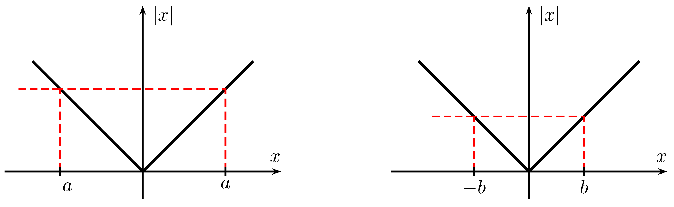
Figure 2.
Definition and properties of information loss. (a) Model for computing the information loss in a memoryless input-output system g. Q is a quantizer with partition ; (b) The information loss of the cascade equals the sum of the individual information losses of the constituent systems.
Figure 2.
Definition and properties of information loss. (a) Model for computing the information loss in a memoryless input-output system g. Q is a quantizer with partition ; (b) The information loss of the cascade equals the sum of the individual information losses of the constituent systems.
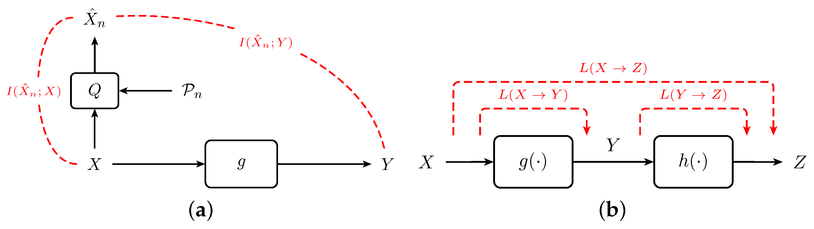
Figure 3.
The center clipper—an example for a system with infinite information loss and infinite information transfer.
Figure 3.
The center clipper—an example for a system with infinite information loss and infinite information transfer.

Figure 4.
Third-order polynomial of Section 5.5. (a) The function and its MAP reconstructor indicated with a thick red line; (b) Information loss as a function of input variance .
Figure 4.
Third-order polynomial of Section 5.5. (a) The function and its MAP reconstructor indicated with a thick red line; (b) Information loss as a function of input variance .

Figure 5.
Constellation diagrams used in the example in Section 5.6: (a) 16-PSK; (b) 16-QAM; and (c) circular 16-QAM.
Figure 5.
Constellation diagrams used in the example in Section 5.6: (a) 16-PSK; (b) 16-QAM; and (c) circular 16-QAM.
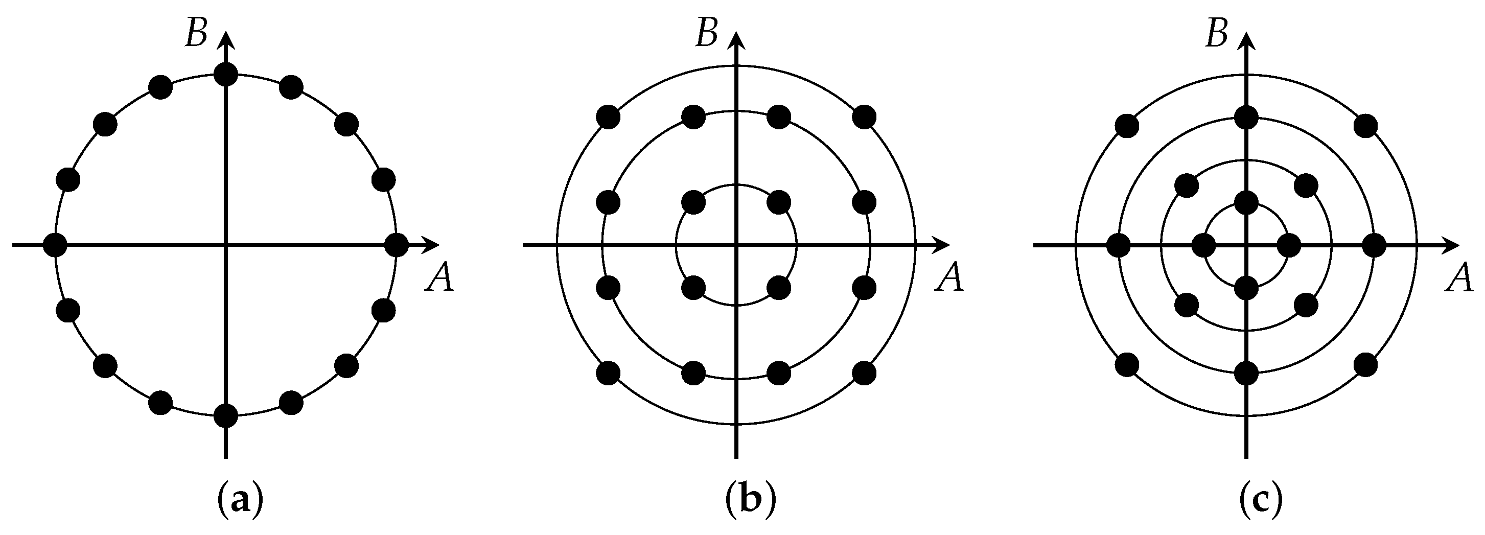
Figure 6.
Mutual information between the constellation points of Figure 5 (normalized to unit energy) and the noisy output of the energy detector . is a Gaussian noise signal with standard deviation σ (see text). Note that the maximum mutual information in the noiseless case is bounded by according to Table 1. The mutual information for 16-PSK with is zero and hence not depicted.


Table 1.
Information loss in the energy detector as a function of the constellation and the integration time .
| TI | 1, 1/2, 1/4 | 1/3 |
|---|---|---|
| 16-PSK | 4 | 1.75 |
| 16-QAM | 2.5 | 2 |
| Circular 16-QAM | 2 | 1.5 |
Table 2.
Comparison of results for some examples from Section 5. While there is a close connection between information loss and the reconstruction error probability (cf. Propositions 8 and 11), there is no apparent connection between information loss and the MSRE—energy and information behave inherently differently.
| Example | MSRE | L(X → Y) | l(X → Y) | Pe |
|---|---|---|---|---|
| , | ∞ | 1 | 100% | |
| Center Clipper, | ∞ | |||
| , | – | ∞ | 100% | |
| , | 1 | 0 | 50% | |
| , X Gaussian | – | Figure 4b | 0 | |
| PCA, | min | ∞ | 100% |
© 2016 by the authors; licensee MDPI, Basel, Switzerland. This article is an open access article distributed under the terms and conditions of the Creative Commons Attribution (CC-BY) license (http://creativecommons.org/licenses/by/4.0/).
Share and Cite
MDPI and ACS Style
Geiger, B.C.; Kubin, G. Information-Theoretic Analysis of Memoryless Deterministic Systems. Entropy 2016, 18, 410. https://doi.org/10.3390/e18110410
AMA Style
Geiger BC, Kubin G. Information-Theoretic Analysis of Memoryless Deterministic Systems. Entropy. 2016; 18(11):410. https://doi.org/10.3390/e18110410
Chicago/Turabian StyleGeiger, Bernhard C., and Gernot Kubin. 2016. "Information-Theoretic Analysis of Memoryless Deterministic Systems" Entropy 18, no. 11: 410. https://doi.org/10.3390/e18110410
Note that from the first issue of 2016, this journal uses article numbers instead of page numbers. See further details here.